
The Numerical Analysis of Non-Newtonian Blood Flow in a Mechanical Heart Valve

Abstract
:1. Introduction
2. Methods
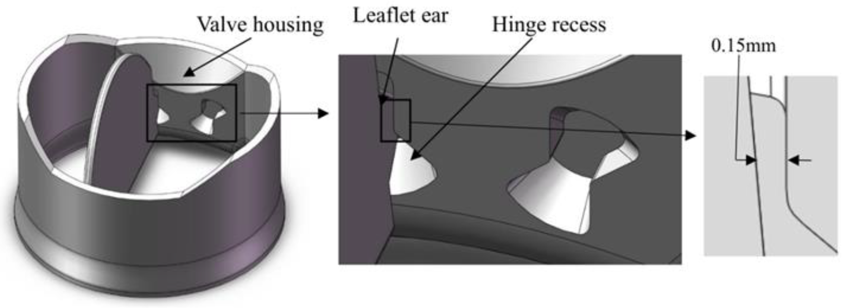
2.1. Geometry
2.2. Governing Equation
2.3. Non-Newtonian Blood Rheologies
2.4. The Simulation Method
- the early accelerating phase;
- mid-acceleration phase;
- peak systole;
- , mid-decelerating phase.
3. Results and Discussion
3.1. The Blood Flow Pattern
3.2. Non-Newtonian Importance Factor
3.3. Wall Shear Stress
4. Conclusions
Author Contributions
Funding
Data Availability Statement
Acknowledgments
Conflicts of Interest
References
- World Health Organization. Cardiovascular Diseases (cvds). 2019. Available online: http://www.who.int/mediacentre/factsheets/fs317/en/index.html (accessed on 7 February 2019).
- Smadi, O.; Hassan, I.; Pibarot, P.; Kadem, L. Numerical and experimental investigations of pulsatile blood flow pattern through a dysfunctional mechanical heart valve. J. Biomech. 2010, 43, 1565–1572. [Google Scholar] [CrossRef]
- Emery, R.W.; Mettler, E.G.O.N.; Nicoloff, D.M. A new cardiac prosthesis: The St. Jude Medical cardiac valve: In vivo results. Circulation 1979, 60, 48–54. [Google Scholar] [CrossRef] [PubMed]
- Gott, V.L.; Alejo, D.E.; Cameron, D.E. Mechanical heart valves: 50 years of evolution. Ann. Thorac. Surg. 2003, 76, S2230–S2239. [Google Scholar] [CrossRef] [PubMed]
- Shahriari, S.; Maleki, H.; Hassan, I.; Kadem, L. Evaluation of shear stress accumulation on blood components in normal and dysfunctional bileaflet mechanical heart valves using smoothed particle hydrodynamics. J. Biomech. 2012, 45, 2637–2644. [Google Scholar] [CrossRef] [PubMed]
- Bessonov, N.; Sequeira, A.; Simakov, S.; Vassilevskii, Y.; Volpert, V. Methods of blood flow modelling. Math. Model. Nat. Phenom. 2016, 11, 1–25. [Google Scholar] [CrossRef] [Green Version]
- Johnston, B.M.; Johnston, P.R.; Corney, S.; Kilpatrick, D. Non-Newtonian blood flow in human right coronary arteries: Steady state simulations. J. Biomech. 2004, 37, 709–720. [Google Scholar] [CrossRef] [Green Version]
- Smadi, O.; Fenech, M.; Hassan, I.; Kadem, L. Flow through a defective mechanical heart valve: A steady flow analysis. Med. Eng. Phys. 2009, 31, 295–305. [Google Scholar] [CrossRef]
- Arzani, A. Accounting for residence-time in blood rheology models: Do we really need non-Newtonian blood flow modelling in large arteries? J. R. Soc. Interface 2018, 15, 20180486. [Google Scholar] [CrossRef] [Green Version]
- Berger, S.A.; Jou, L.D. Flows in stenotic vessels. Annu. Rev. Fluid Mech. 2000, 32, 347–382. [Google Scholar] [CrossRef]
- Merrill, E.W.; Gilliland, E.R.; Margetts, W.G.; Hatch, F.T. Rheology of human blood and hyperlipemia. J. Appl. Physiol. 1964, 19, 493–496. [Google Scholar] [CrossRef]
- Phillips, W.M.; Deutsch, S. Toward a constitutive equation for blood. Biorheology 1975, 12, 383–389. [Google Scholar] [CrossRef] [PubMed]
- Yun, B.M.; McElhinney, D.B.; Arjunon, S.; Mirabella, L.; Aidun, C.K.; Yoganathan, A.P. Computational simulations of flow dynamics and blood damage through a bileaflet mechanical heart valve scaled to pediatric size and flow. J. Biomech. 2014, 47, 3169–3177. [Google Scholar] [CrossRef] [PubMed] [Green Version]
- Yeh, H.H.; Barannyk, O.; Grecov, D.; Oshkai, P. The influence of hematocrit on the hemodynamics of artificial heart valve using fluid-structure interaction analysis. Comput. Biol. Med. 2019, 110, 79–92. [Google Scholar] [CrossRef] [PubMed]
- Campo-Deaño, L.; Dullens, R.P.; Aarts, D.G.; Pinho, F.T.; Oliveira, M.S. Viscoelasticity of blood and viscoelastic blood analogues for use in polydymethylsiloxane in vitro models of the circulatory system. Biomicrofluidics 2013, 7, 034102. [Google Scholar] [CrossRef] [Green Version]
- Zupančič Valant, A.; Žiberna, L.; Papaharilaou, Y.; Anayiotos, A.; Georgiou, G.C. The influence of temperature on rheological properties of blood mixtures with different volume expanders—Implications in numerical arterial hemodynamics simulations. Rheol. Acta 2011, 50, 389–402. [Google Scholar] [CrossRef]
- De Vita, F.; De Tullio, M.D.; Verzicco, R. Numerical simulation of the non-Newtonian blood flow through a mechanical aortic valve. Theor. Comput. Fluid Dyn. 2016, 30, 129–138. [Google Scholar] [CrossRef]
- Moradicheghamahi, J.; Sadeghiseraji, J.; Jahangiri, M. Numerical solution of the Pulsatile, non-Newtonian and turbulent blood flow in a patient specific elastic carotid artery. Int. J. Mech. Sci. 2019, 150, 393–403. [Google Scholar] [CrossRef]
- Doost, S.N.; Zhong, L.; Su, B.; Morsi, Y.S. The numerical analysis of non-Newtonian blood flow in human patient-specific left ventricle. Comput. Methods Programs Biomed. 2016, 127, 232–247. [Google Scholar] [CrossRef]
- Nadarajah, S.K.; McMullen, M.S.; Jameson, A. Aerodynamic shape optimization for unsteady three-dimensional flows. Int. J. Comput. Fluid Dyn. 2006, 20, 533–548. [Google Scholar] [CrossRef]
- Weddell, J.C.; Kwack, J.; Imoukhuede, P.I.; Masud, A. Hemodynamic analysis in an idealized artery tree: Differences in wall shear stress between Newtonian and non-Newtonian blood models. PLoS ONE 2015, 10, e0124575. [Google Scholar] [CrossRef]
- Caballero, A.D.; Laín, S. Numerical simulation of non-Newtonian blood flow dynamics in human thoracic aorta. Comput. Methods Biomech. Biomed. Eng. 2015, 18, 1200–1216. [Google Scholar] [CrossRef] [PubMed]
- Hanafizadeh, P.; Mirkhani, N.; Davoudi, M.R.; Masouminia, M.; Sadeghy, K. Non-newtonian blood flow simulation of diastolic phase in bileaflet mechanical heart valve implanted in a realistic aortic root containing coronary arteries. Artif. Organs 2016, 40, E179–E191. [Google Scholar] [CrossRef] [PubMed]
- Abbas, S.S.; Nasif, M.S.; Al-Waked, R.; Meor Said, M.A. Numerical investigation on the effect of bileaflet mechanical heart valve’s implantation tilting angle and aortic root geometry on intermittent regurgitation and platelet activation. Artif. Organs 2020, 44, E20–E39. [Google Scholar] [CrossRef] [PubMed]
- Choi, C.R.; Kim, C.N. Analysis of blood flow interacted with leaflets in MHV in view of fluid-structure interaction. KSME Int. J. 2001, 15, 613–622. [Google Scholar] [CrossRef]
- Kadhim, S.K.; Nasif, M.S.; Al-Kayiem, H.H.; Al-Waked, R. Computational fluid dynamics simulation of blood flow profile and shear stresses in bileaflet mechanical heart valve by using monolithic approach. Simulation 2018, 94, 93–104. [Google Scholar] [CrossRef] [Green Version]
- Forsyth, A.M.; Wan, J.; Owrutsky, P.D.; Abkarian, M.; Stone, H.A. Multiscale approach to link red blood cell dynamics, shear viscosity, and ATP release. Proc. Natl. Acad. Sci. USA 2011, 108, 10986–10991. [Google Scholar] [CrossRef] [Green Version]
- Wagner, C.; Steffen, P.; Svetina, S. Aggregation of red blood cells: From rouleaux to clot formation. Comptes Rendus Phys. 2013, 14, 459–469. [Google Scholar] [CrossRef] [Green Version]
- Hellmeier, F.; Nordmeyer, S.; Yevtushenko, P.; Bruening, J.; Berger, F.; Kuehne, T.; Goubergrits, L.; Kelm, M. Hemodynamic evaluation of a biological and mechanical aortic valve prosthesis using patient-specific MRI-based CFD. Artif. Organs 2018, 42, 49–57. [Google Scholar] [CrossRef]
- Karimi, S.; Dabagh, M.; Vasava, P.; Dadvar, M.; Dabir, B.; Jalali, P. Effect of rheological models on the hemodynamics within human aorta: CFD study on CT image-based geometry. J. Non Newton. Fluid Mech. 2014, 207, 42–52. [Google Scholar] [CrossRef]
- Jahangiri, M.; Saghafian, M.; Sadeghi, M.R. Numerical simulation of non-Newtonian models effect on hemodynamic factors of pulsatile blood flow in elastic stenosed artery. J. Mech. Sci. Technol. 2017, 31, 1003–1013. [Google Scholar] [CrossRef]
- Jahangiri, M.; Saghafian, M.; Sadeghi, M.R. Numerical study of turbulent pulsatile blood flow through stenosed artery using fluid-solid interaction. Comput. Math. Methods Med. 2015, 2015, 515613. [Google Scholar] [CrossRef] [PubMed] [Green Version]
- Yin, W.; Gallocher, S.; Pinchuk, L.; Schoephoerster, R.T.; Jesty, J.; Bluestein, D. Flow-induced platelet activation in a St. Jude mechanical heart valve, a trileaflet polymeric heart valve, and a St. Jude tissue valve. Artif. Organs 2005, 29, 826–831. [Google Scholar] [CrossRef] [PubMed]
- Mirkhani, N.; Davoudi, M.R.; Hanafizadeh, P.; Javidi, D.; Saffarian, N. On-X heart valve prosthesis: Numerical simulation of hemodynamic performance in accelerating systole. Cardiovasc. Eng. Technol. 2016, 7, 223–237. [Google Scholar] [CrossRef] [PubMed]
- De Tullio, M.D.; Cristallo, A.; Balaras, E.; Verzicco, R. Direct numerical simulation of the pulsatile flow through an aortic bileaflet mechanical heart valve. J. Fluid Mech. 2009, 622, 259–290. [Google Scholar] [CrossRef] [Green Version]
- Akutsu, T.; Matsumoto, A. Influence of three mechanical bileaflet prosthetic valve designs on the three-dimensional flow field inside a simulated aorta. J. Artif. Organs 2010, 13, 207–217. [Google Scholar] [CrossRef]
- Onel, H.C.; Tuncer, I.H. A comparative study of wake interactions between wind-aligned and yawed wind turbines using LES and actuator line models. J. Phys. Conf. Ser. 2020, 1618, 062009. [Google Scholar] [CrossRef]
- Zakaria, M.S.; Ismail, F.; Tamagawa, M.; Aziz, A.F.A.; Wiriadidjaja, S.; Basri, A.A.; Ahmad, K.A. Review of numerical methods for simulation of mechanical heart valves and the potential for blood clotting. Med. Biol. Eng. Comput. 2017, 55, 1519–1548. [Google Scholar] [CrossRef]
- O’Callaghan, S.; Walsh, M.; McGloughlin, T. Numerical modelling of Newtonian and non-Newtonian representation of blood in a distal end-to-side vascular bypass graft anastomosis. Med. Eng. Phys. 2006, 28, 70–74. [Google Scholar] [CrossRef]
- Kim, S.K. Collective viscosity model for shear thinning polymeric materials. Rheol. Acta 2020, 59, 63–72. [Google Scholar] [CrossRef]
- Cho, Y.I.; Kensey, K.R. Effects of the non-Newtonian viscosity of blood on flows in a diseased arterial vessel. Part 1: Steady flows. Biorheology 1991, 28, 241–262. [Google Scholar] [CrossRef]
- Shibeshi, S.S.; Collins, W.E. The rheology of blood flow in a branched arterial system. Appl. Rheol. 2005, 15, 398–405. [Google Scholar] [CrossRef] [PubMed]
- Borazjani, I.; Ge, L.; Sotiropoulos, F. Curvilinear immersed boundary method for simulating fluid structure interaction with complex 3D rigid bodies. J. Comput. Phys. 2008, 227, 7587–7620. [Google Scholar] [CrossRef] [PubMed] [Green Version]
- Simon, H.A.; Ge, L.; Sotiropoulos, F.; Yoganathan, A.P. Simulation of the three-dimensional hinge flow fields of a bileaflet mechanical heart valve under aortic conditions. Ann. Biomed. Eng. 2010, 38, 841–853. [Google Scholar] [CrossRef] [PubMed] [Green Version]
- Prakash, S.; Ethier, C.R. Requirements for mesh resolution in 3D computational hemodynamics. J. Biomech. Eng. 2001, 123, 134–144. [Google Scholar] [CrossRef] [PubMed]
- Grigioni, M.; Daniele, C.; D’Avenio, G.; Barbaro, V. The influence of the leaflets’ curvature on the flow field in two bileaflet prosthetic heart valves. J. Biomech. 2001, 34, 613–621. [Google Scholar] [CrossRef]
- Khalili, F.; Gamage, P.; Sandler, R.H.; Mansy, H.A. Adverse hemodynamic conditions associated with mechanical heart valve leaflet immobility. Bioengineering 2018, 5, 74. [Google Scholar] [CrossRef] [Green Version]
- Ge, L.; Jones, S.C.; Sotiropoulos, F.; Healy, T.M.; Yoganathan, A.P. Numerical simulation of flow in mechanical heart valves: Grid resolution and the assumption of flow symmetry. J. Biomech. Eng. 2003, 125, 709–718. [Google Scholar] [CrossRef]
- Smadi, O.; Garcia, J.; Pibarot, P.; Gaillard, E.; Hassan, I.; Kadem, L. Accuracy of Doppler-echocardiographic parameters for the detection of aortic bileaflet mechanical prosthetic valve dysfunction. Eur. Heart J. Cardiovasc. Imaging 2014, 15, 142–151. [Google Scholar] [CrossRef] [Green Version]
- Zhang, J.B.; Kuang, Z.B. Study on blood constitutive parameters in different blood constitutive equations. J. Biomech. 2000, 33, 355–360. [Google Scholar] [CrossRef]


| Model | Viscosity | Parameters |
|---|---|---|
| Modified Power-law (PL) [39] | | |
| Carreau [25] | ||
| Carreau–Yasuda (CY) [40] | ||
| Casson [16] | ||
| Modified Casson [7] | ||
| Cross [21] | ||
| Modified Cross [21] | ||
| Powell–Eyring (PE) [41] | ||
| Modified Powell–Eyring (Md PE) [41] | ||
| K–L [42] | |
| Calculated Time (s) | 0.03 | 0.09 | 0.19 | 0.29 | |
|---|---|---|---|---|---|
| Carreau | WL | 0.054 | 0.033 | 0.023 | 0.034 |
| HR | 0.474 | 0.115 | 0.105 | 0.321 | |
| CY | WL | 0.014 | 0.010 | 0.008 | 0.010 |
| HR | 0.106 | 0.038 | 0.036 | 0.081 | |
| Casson | WL | 0.073 | 0.064 | 0.059 | 0.065 |
| HR | 0.406 | 0.262 | 0.256 | 0.353 | |
| Md Casson | WL | 0.039 | 0.026 | 0.017 | 0.025 |
| HR | 0.338 | 0.085 | 0.075 | 0.254 | |
| Cross | WL | 0.037 | 0.009 | 0.006 | 0.014 |
| HR | 0.395 | 0.029 | 0.028 | 0.209 | |
| Md Cross | WL | 0.059 | 0.037 | 0.026 | 0.038 |
| HR | 0.505 | 0.131 | 0.120 | 0.340 | |
| K–L | WL | 0.021 | 0.016 | 0.013 | 0.016 |
| HR | 0.147 | 0.062 | 0.059 | 0.103 | |
| PL | WL | 0.034 | 0.020 | 0.009 | 0.018 |
| HR | 0.366 | 0.051 | 0.043 | 0.242 | |
| PE | WL | 0.036 | 0.018 | 0.012 | 0.020 |
| HR | 0.354 | 0.060 | 0.054 | 0.250 | |
| Md PE | WL | 0.049 | 0.024 | 0.014 | 0.025 |
| HR | 0.489 | 0.073 | 0.064 | 0.309 | |
| Calculate Region | Wall and Leaflet (Pa) | Hinge Region (Pa) | |||||||
|---|---|---|---|---|---|---|---|---|---|
| t (s) | 0.030 | 0.090 | 0.190 | 0.290 | 0.030 | 0.090 | 0.190 | 0.290 | |
| Newtonian | Max_WSS | 16.909 | 99.636 | 223.166 | 74.815 | 8.398 | 30.684 | 50.804 | 8.555 |
| Agv_WSS | 2.043 | 6.483 | 13.840 | 5.908 | 1.412 | 6.587 | 8.220 | 1.283 | |
| Carreau | Max_WSS | 17.147 | 101.630 | 227.185 | 76.133 | 8.080 | 31.633 | 49.959 | 8.994 |
| Agv_WSS | 2.220 | 6.761 | 14.067 | 5.957 | 1.466 | 6.871 | 8.490 | 1.328 | |
| CY | Max_WSS | 17.074 | 101.260 | 226.726 | 75.471 | 8.190 | 31.361 | 50.267 | 8.873 |
| Agv_WSS | 2.149 | 6.654 | 13.987 | 5.891 | 1.443 | 6.763 | 8.381 | 1.324 | |
| Casson | Max_WSS | 28.803 | 110.301 | 253.279 | 81.849 | 9.114 | 34.399 | 47.749 | 9.488 |
| Agv_WSS | 2.372 | 7.281 | 14.923 | 6.012 | 1.514 | 7.386 | 9.132 | 1.399 | |
| Md Casson | Max_WSS | 17.428 | 104.614 | 236.702 | 78.006 | 8.928 | 31.720 | 51.595 | 8.656 |
| Agv_WSS | 2.171 | 6.514 | 14.069 | 6.015 | 1.462 | 6.611 | 8.234 | 1.349 | |
| Cross | Max_WSS | 17.091 | 101.063 | 226.584 | 75.627 | 8.387 | 31.170 | 50.381 | 8.742 |
| Agv_WSS | 2.083 | 6.572 | 13.954 | 5.736 | 1.422 | 6.678 | 8.305 | 1.273 | |
| Md Cross | Max_WSS | 17.180 | 101.797 | 227.459 | 76.376 | 8.046 | 31.742 | 49.824 | 9.023 |
| Agv_WSS | 2.244 | 6.802 | 14.105 | 6.020 | 1.475 | 6.912 | 8.533 | 1.342 | |
| K–L | Max_WSS | 17.140 | 101.419 | 227.104 | 75.268 | 8.293 | 31.406 | 50.172 | 8.886 |
| Agv_WSS | 2.134 | 6.661 | 14.020 | 5.874 | 1.438 | 6.766 | 8.400 | 1.348 | |
| PL | Max_WSS | 17.067 | 101.089 | 226.558 | 75.586 | 8.754 | 31.193 | 50.318 | 8.893 |
| Agv_WSS | 2.096 | 6.574 | 13.947 | 5.798 | 1.425 | 6.681 | 8.288 | 1.280 | |
| PE | Max_WSS | 17.769 | 101.185 | 226.638 | 74.923 | 8.864 | 31.302 | 50.318 | 8.830 |
| Agv_WSS | 2.134 | 6.628 | 13.970 | 5.836 | 1.539 | 6.738 | 8.353 | 1.397 | |
| Md PE | Max_WSS | 17.066 | 101.223 | 226.640 | 75.288 | 8.183 | 31.346 | 50.297 | 8.886 |
| Agv_WSS | 2.154 | 6.645 | 13.971 | 5.873 | 1.446 | 6.757 | 8.365 | 1.342 | |
Disclaimer/Publisher’s Note: The statements, opinions and data contained in all publications are solely those of the individual author(s) and contributor(s) and not of MDPI and/or the editor(s). MDPI and/or the editor(s) disclaim responsibility for any injury to people or property resulting from any ideas, methods, instructions or products referred to in the content. |
© 2022 by the authors. Licensee MDPI, Basel, Switzerland. This article is an open access article distributed under the terms and conditions of the Creative Commons Attribution (CC BY) license (https://creativecommons.org/licenses/by/4.0/).
Share and Cite
Chen, A.; Basri, A.A.; Ismail, N.B.; Ahmad, K.A. The Numerical Analysis of Non-Newtonian Blood Flow in a Mechanical Heart Valve. Processes 2023, 11, 37. https://doi.org/10.3390/pr11010037
Chen A, Basri AA, Ismail NB, Ahmad KA. The Numerical Analysis of Non-Newtonian Blood Flow in a Mechanical Heart Valve. Processes. 2023; 11(1):37. https://doi.org/10.3390/pr11010037
Chicago/Turabian StyleChen, Aolin, Adi Azriff Basri, Norzian Bin Ismail, and Kamarul Arifin Ahmad. 2023. "The Numerical Analysis of Non-Newtonian Blood Flow in a Mechanical Heart Valve" Processes 11, no. 1: 37. https://doi.org/10.3390/pr11010037