1. Introduction
The environmental aspect of the industry in today’s world is increasingly becoming a concern among producers and clients. It is expected that the product will not only be reasonably priced and of high quality, but also that it will have a low environmental impact, either due to the materials used or due to the manufacturing process [
1].
Industry 4.0 focuses on the digitalization and optimization of processes, through the interaction of different system components, often utilizing technologies such as the Internet of Things (IoT) or Cyber-Physical Production Systems (CPPS) to achieve the desired results. Nevertheless, the usage of such systems is often not enough, as with the arrival of mass customization and ever-increasing difficulties in optimizing the processes, especially with the high consumption of raw resources, energy and information, the process become increasingly more difficult to optimize as more variables are put in place and more processes differ from product to product. It is necessary to better these systems to tackle with the new difficulties of increasing the process making and product personalization efficiency of the Industry 4.0 paradigm. As society becomes more aware of the problem, new solutions start to be developed with the idea of mitigating the losses and optimizing the processes [
2].
With the present focus on energy reduction and efficiency, there are several processes that help reduce or optimize energy consumption. The solution is frequently a combination of methods based on passive and active energy consumption reduction. The passive energy consumption reduction method does not actively need action to effectively reduce the energy consumption, for example, the Trombe wall, lightweight concrete wall, natural ventilation, roof greening and architectural design [
3]. On the other hand, the active energy consumption optimization methods actively need to consider, either by software or human resources, the energy consumption data for their decisions, for example, by minimizing the time of support activities that do not create value, updating to more electrical efficiency components and integrating high-level production management decision with energy data such as production planning and scheduling, demand response, machine configuration and logistics [
4]. Furthermore, this energy consumption must also be reflected in an optimization of the industrial manufacturing process, resulting in a decrease in expenses on the electricity bill.
This work focuses on the use of a machine learning (ML) cloud-based application to optimize the energy consumption of the manufacturing process with regards to the welding of automotive parts in compliance of the Ford and Volkswagen (VW) industrial parameters. To be able to achieve this goal, a brief introduction of the cloud applications in the industry and ML for energy management is conducted in the next section.
1.1. Cloud Applications
In Industry 4.0, the utilization of cloud-based applications is becoming a staple, with programs running in a cloud environment able to be more easily accessed by all interested parties, be they humans, machines or software programs. In the literature, several examples can be found of software applications running in the cloud that add value to the systems or products of a factory. Some of them utilize software to monitor and predict or track the state and maintenance of the equipment [
5]. Others use this cloud-based software to control the schedule, as it is one of the most important areas of the manufacturing process that is often conducted in a rudimentary manual way [
6]. A good approach to improving the way scheduling is conducted is implementing service-based cloud software, which helps the whole factory easily implement, modify or adjust the production schedule [
7,
8]. An additional use of the cloud technology is the utilization of such software for collaboration in new ways. The software being in the cloud allows an easier approach to working with manufacturing as a service, not only with the final client but also in collaboration with other factories [
9,
10]. Another growing use is the fact that the cloud-based approach facilitates the usage and collection of elevated volumes of information. This approach allows the centralization of the data to a specific piece of software or specific database, allowing it to be worked on or correlated with other data or events [
11]. In [
12], the authors propose an automated system using Artificial Intelligence (AI) connected to an online shopping platform that allows the robot to pick the list of products demanded in by the costumer, revealing a flow of data between a cloud platform and a robot, also allowing the delivery of some information back from the robot to the cloud-base management platform. Last comes the utilization of such software to help in the management of resources. An example comes from the usage of cloud services integrated with additive and subtractive manufacturing to boost resource efficiency [
13].
As seen previously, cloud-based applications can help optimize the production and processes of the industry, and it can be an important tool to minimize the production cost, in this case by optimizing the energy consumption for the production. There are already articles demonstrating the usage of cloud-based software regarding the optimization of energy consumption [
14,
15]; nevertheless, it usually does not demonstrate all the processes from the shopfloor to the cloud-based applications, besides having a clear and real-world test scenario regarding the usage of such methods.
1.2. Machine Learning for Energy Consumption Prediction and Management
We are currently in the era of IoT and Big Data, that is, at every moment, huge amounts of data are produced all over the world, far beyond what a human can process. As a result of this constant torrent of information, methods of data analysis emerge, which is what ML provides. ML can be broadly defined as a subfield of AI, which gives certain machines the ability to learn, without being explicitly programmed to, from computational methods that use “experience” (training data), such as information and/or past events, to improve performance or to make accurate predictions [
16,
17,
18].
The evolution in technology leads large organizations to entrust the control and monitoring of data to ML algorithms. Basically, ML can be applied to large volumes of data to produce deeper insights and improve decision-making, so that industries can improve their operations and competitiveness. There are many ML-based functionalities used these days.
According to [
19], there are five potential game changing use cases from across industries that uses Big Data applications for ML techniques: (a) condition monitoring, (b) quality diagnostics, (c) energy optimization, (d) demand prediction, and (e) propensity to buy.
Focusing on topic energy optimization, which is one of the issues described in this document, in the industrial sector, the continuous increase in energy consumption and the scarcity of non-renewable resources force several industrial entities to search for new methods to improve energy management and, hence, saving costs. In an interesting review of energy management in the industry provided by [
20], the authors identified five high-level energy efficiency functions, and their specific objectives, using ML tools, namely: (a) Estimation: (i) energy efficiency metrics resolution; (ii) benchmark and baseline identification. (b) Prediction: (i) input-output model development; (ii) energy consumption trend prediction. (c) Analysis: (i) operating modes classification and identification; (ii) identification of saving potentials and energy savings; (iii) identification of key variables for energy efficiency; (iv) quantification of energy consumption per product. (d) Optimization: (i) corrective actions; (ii) optimal scheduling; (iii) optimal control; (iv) optimal process settings; (v) robustness. (e) Technology and scale: (i) technology assessment; (ii) scale assessment.
Currently, predictive analytics are seen as a game changer for the industry. Due to the importance of optimizing energy consumption, many researchers are exploring the use of different types of ML algorithms to forecast energy consumption. Some examples are Decision trees and Random Forest, Linear and non-linear regression and Artificial Neural Networks (ANN) [
21]. For example, the authors in [
22] studied various models to predict energy consumption for a smart small-scale steel industry, namely: general linear regression, decision tree-based classification and regression trees, Random Forest, Support Vector Machine with a radial basis kernel, K-nearest neighbors and CUBIST. In [
23], the authors proposed an hourly building energy prediction model using Random Forest and compared it with regression tree and Support Vector Regression. In [
24], an intelligent reasoning system is presented, featuring energy consumption prediction and optimization of cutting parameters in milling process. ANN and Intelligent Case Based Reasoning (ICBR) are used for providing accurate estimation of cutting power. The authors of [
25] designed a supervised ML-approached analytic modeling to predict a sustainable performance for power consumption in the metal cutting industry. In [
26], a predictive approach was proposed using deep learning-driven techniques to reduce energy consumption in additive manufacturing.
1.3. This Work’s Contribution
This specific work’s contributions revolve around the Introsys company and the necessity to improve the energy efficiency of the production. Having an already-established infrastructure of collecting and storing production and energy consumption data [
27], the next logical step is to expand upon what is already built and develop new systems cable of helping the shopfloor managers make the best decisions regarding the scheduling of the production and the correct functioning of the machinery.
Building upon the aforementioned infrastructure, new cloud tools were developed to provide easy access across the whole plant the ML predictive models. Moreover, the data model was improved to accommodate the predictive model’s necessary inputs and register the outputs and finally the improve of the HMI, to accommodate the ML predictive models output and facilitate the view of the relevant data either by the shopfloor worker or the manager.
Regarding the predictive analysis, two ML algorithms (Linear regression and Random Forest) are used to create the ML predictive models to create energy profiles of two robotics cells (Ford and VW) and to predict the energy consumption of these same cells.
This approach will allow industrial entities to have a better view of their energy consumption, helping them to lower costs and have a better decision-making, thus achieving both sustainability and production goals.
2. Materials and Methods
This section contains the methods, specifications, materials and approaches of the work done to demonstrate the implementation and utility of the presented work. First, the system architecture is presented, using a middleware in the cloud responsible for being the bridge between the communication among different cloud applications (e.g., prediction software, database and data visualization software) or shopfloor machinery. Second, to achieve this setup, a deployment of the cloud environment, made with containers, was implemented. This deployment was made with the software portainer.io using Docker containers, where different containers represent the different software deployed and one of these containers included the prediction software responsible for the energy consumption prediction of the given machines. ML was used to train the prediction software, utilizing data available from previous productions in the robotic cells, and correlating it with the energetic consumption, ultimately making the prediction models.
Despite the architecture and methodology being valid for the complete shopfloor processes, for demonstration purposes, it was used two robotic cells. The use of any another machine from the shopfloor process will utilize the same principles demonstrated for these two robotic cells.
2.1. System Architecture
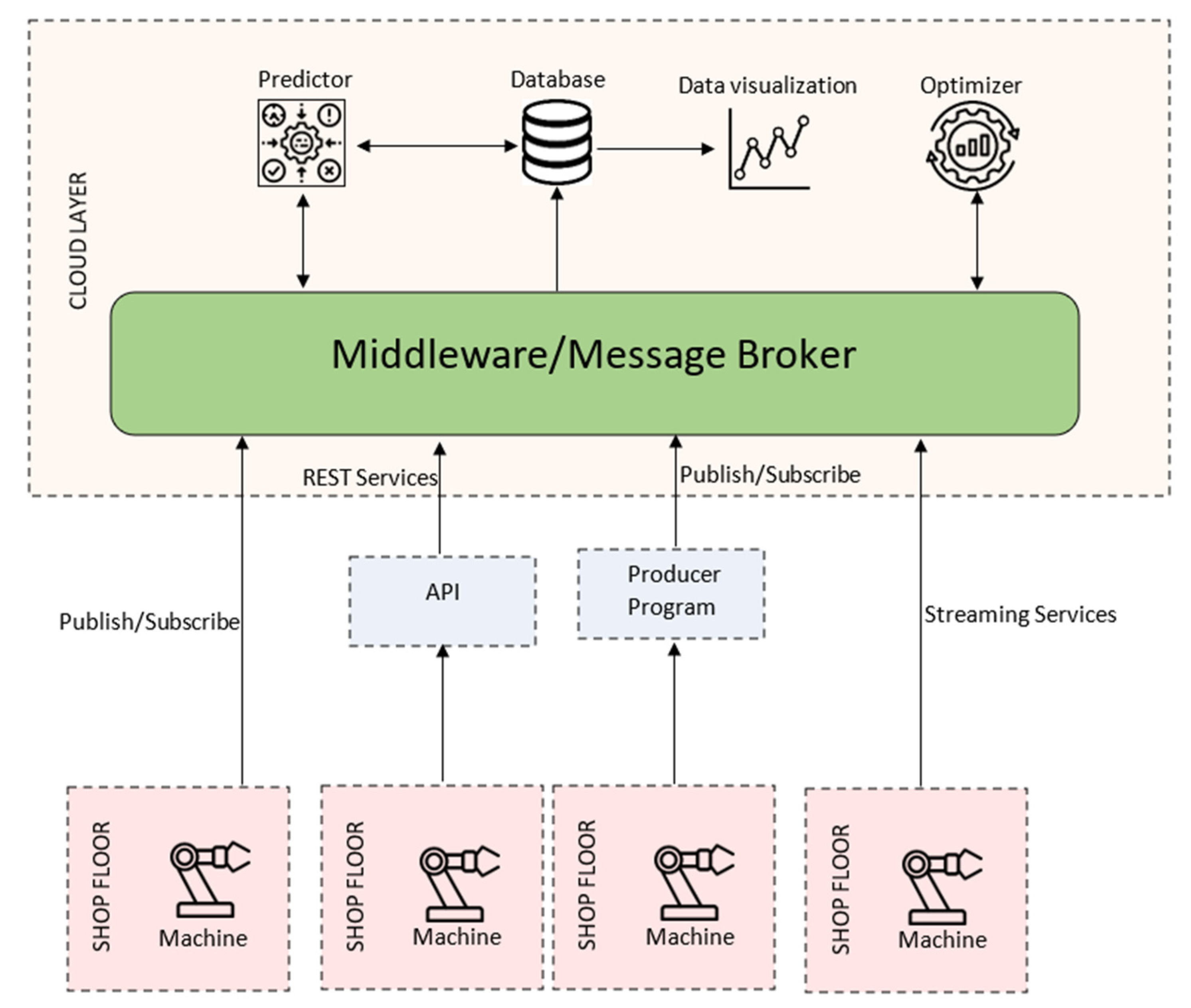
The architecture used for the use case demonstration in this paper is presented in
Figure 1. The presented architecture can be divided into three focus areas: the shopfloor, the middleware and the cloud software (applications).
On the shopfloor, there is a representation of the machinery present in a common producing factory. This symbolizes the types of machines with their different and respective categories. The main restriction, however, is that it should be possible to extract data from the machine either by having external sensors/devices that can extract the state and metrics of the machine or by internally the machine be able to communicate these states and metrics to external entities. The communication is also highlighted here, where different machines can communicate with the middleware through different methods, either by dedicated libraries allowing the more technologically advanced machines to be able to directly connect to the middleware through publish/subscribe or a streaming service approach. For the rest of the machines, an auxiliar program can collect the data and publish in the middleware and, finally, the middleware can also provide a REST API (Application Programming Interface) so that some machines, sensors or programs can communicate through HTTP (Hypertext Transfer Protocol), collecting or sending data to the middleware.
After the data are extracted, they are sent to the middleware that is responsible for handling all the communications from the shopfloor machines and between the cloud applications. The middleware based on a publish/subscribe approach allows the introduction of several new and different machines without the need for complicated integration of all the other machines. The new machines need only to connect with the middleware and, after the connection is successful, subscribe and publish to the relevant topics. The same can be said for cloud applications, as the new software only needs to be able to communicate with the middleware, using one of the mechanisms at its disposal, and utilize the available data to execute the application process and then publish the results. The machines can also receive and publish different types of data, granting other machines or software the possibility to use this data as they deem fit and change parameters or tasks as the data changes. The approach of publish/subscribe allow one of the main advantages of the usage of the architecture, being the scalability of the shopfloor, machinery or local and cloud-software only by needing the new systems to connect to the middleware.
Finally, the cloud applications, use the data at their disposal to generate information or knowledge, which is then stored in a database or passed as parameters to the shopfloor. These applications can vary in complexity and usefulness, as they can be databases, optimization software, data visualization applications and data processing software, among many other useful applications relevant to the industrial environment.
This architecture was designed with a focus on the energetic optimization of a company, as several machines produce and send energetic consumption data to the cloud, meant to be processed and create metrics to visualize the energy consumption and alert in the event of abnormal energy consumption. A cloud-based optimization software can also be used to direct production and optimize the velocity in terms of energy consumption or delivery times.
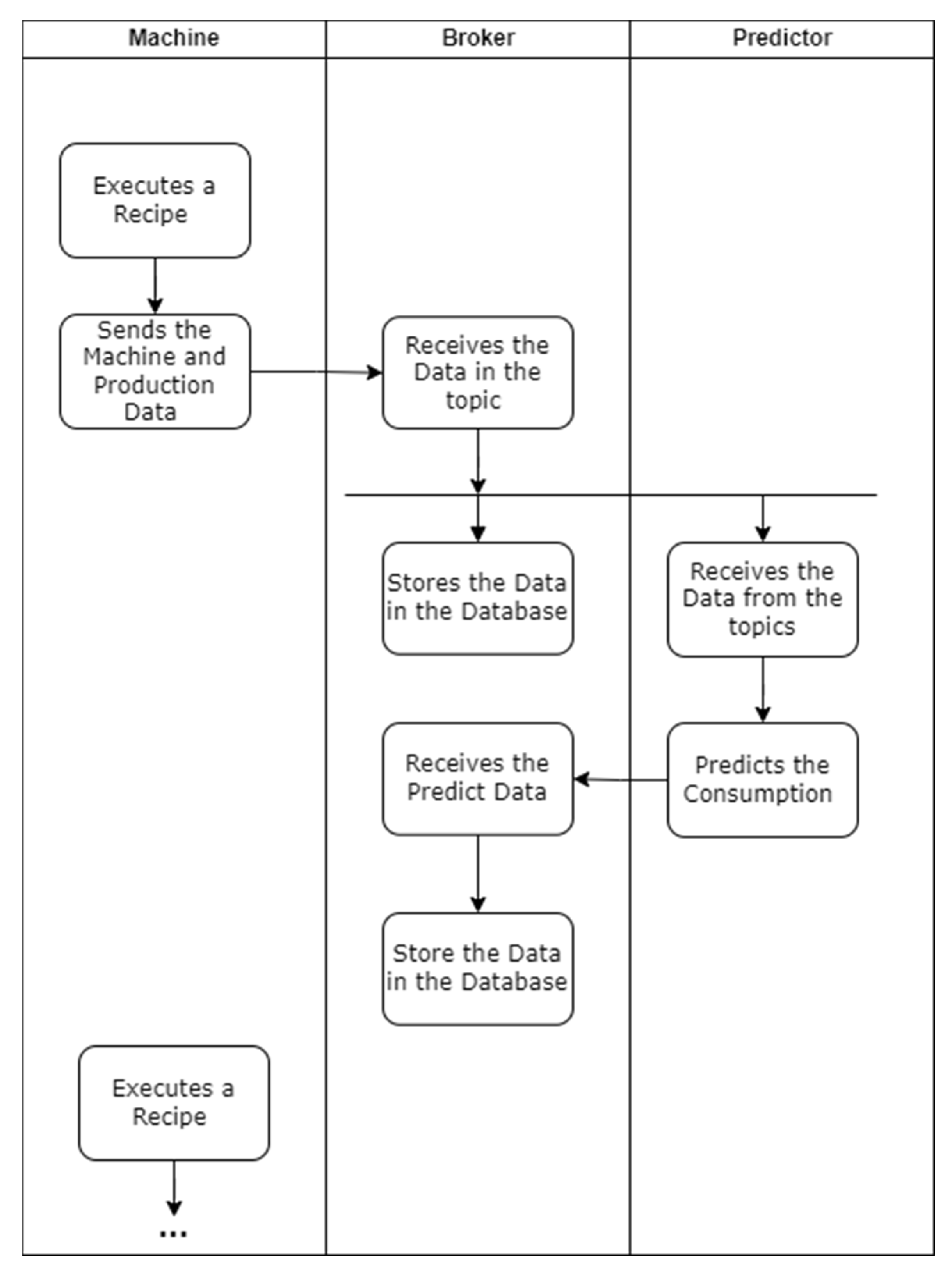
Regarding the communication between the different devices of the architecture, an activity diagram was created, see
Figure 2. The diagram, which will support the implementation, demonstrates how the different systems communicate with each other. It can be seen in the diagram that the communication between the shopfloor machinery starts after the end of production, and all the relevant metrics are sent to the message broker. The message broker not only stores the data in the database but also allows other programs to subscribe to the topic and receive the subscribed metrics. Finally, the communication between the message broker and the predictor is highlighted. After receiving the data, the predictor utilizes the input machinery data to predict the energy consumption. Then, after concluding the prediction, the software sends the new data to another topic of the message broker with the objective of storing the data in the database.
2.2. Demonstration Scenario
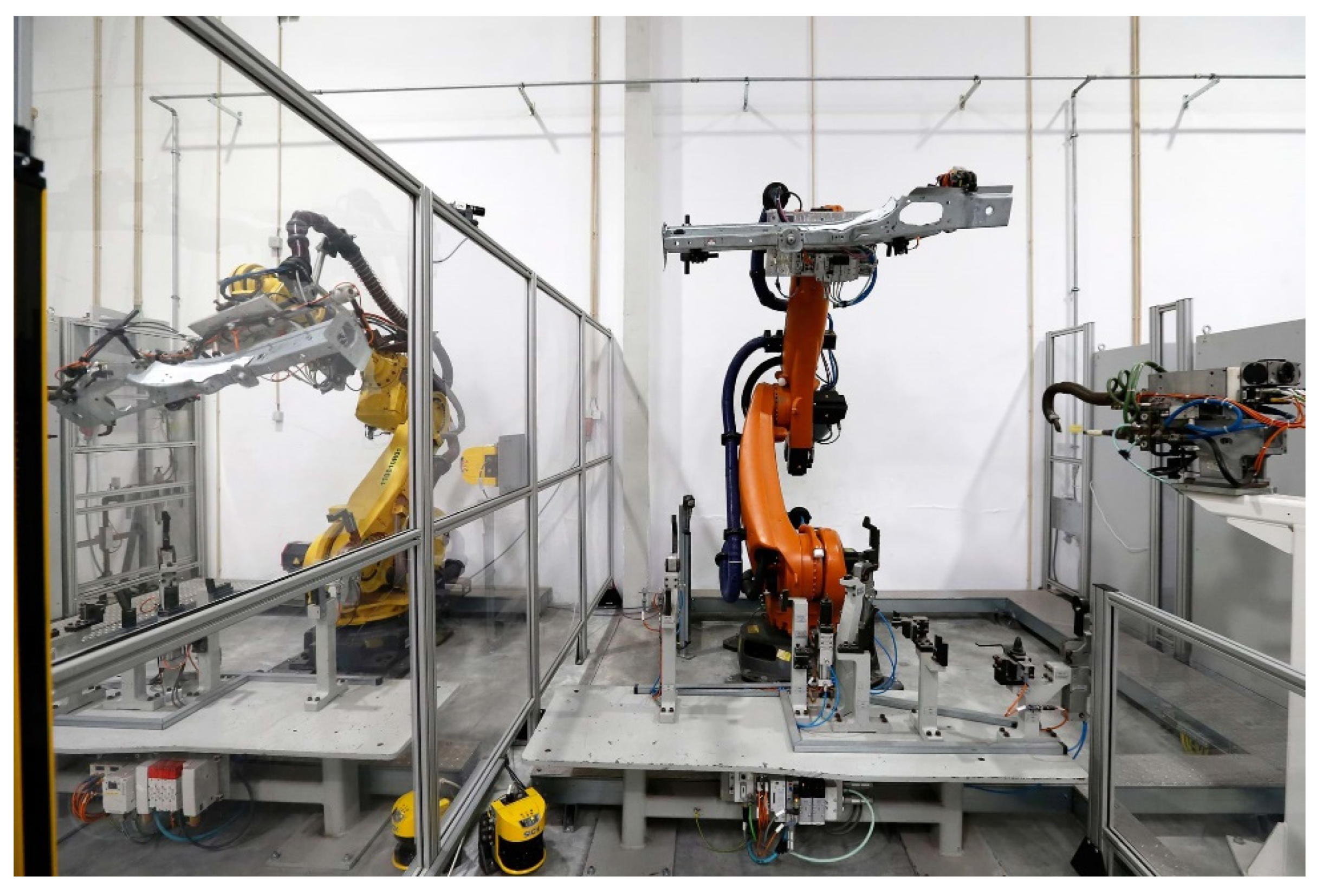
The demonstration scenario for the beforementioned solution was based on the current robotic assembly cells used in Introsys SA installations, in Quinta do Anjo, Portugal, for testing and training (
Figure 3). These cells were first introduced during Proflex project, with the main objective of closing the gap between academia and industrial manufacturers by providing pilots, which represent the reality of actual production lines regarding equipment, safety and control standards used and approved by the automotive industry, yet they do not take in to account the major drawbacks and risks of cells imbedded in production lines, where changes and new integrations cannot be made with ease due to the risk of causing disruptions to the production line itself and its respective value chain. Each one implements several spot-welding processes and comprises a 6-DoF robotic arm with a custom gripper attached, a fixture into which the operator inserts and removes the product before and after the process, a stationary welding gun and several sensors to monitor energy consumption for the different components mentioned.
The workstations, for each cell, were designed to automatically manipulate and simulate spot welding processes on a side member car part, and both can perform the exact same processes. Nevertheless, the main difference between them is the compliance with two different major car manufacturers standards, which rule the adoption of equipment suppliers, control systems, safety approaches, programming methods and tools. Bearing this in mind, the demonstration scenario mentioned provides the ideal conditions to show the interoperability of the system when deployed in actual execution processes from different end-users. Additionally, with both cells having multiple welding programs available, they can handle multiple product variants (types) and the process may be described as follows: (i) the operator deploys the car part on the fixture; (ii) the robot moves the part from the fixture to a stationary welding gun; (iii) the part is moved to a vision-based quality inspection system; (iv) the part is moved back to the fixture. When simulating spot welding, several different welding spots need to be set; therefore, the robot needs to reposition the product in relation to the welding gun for each spot.
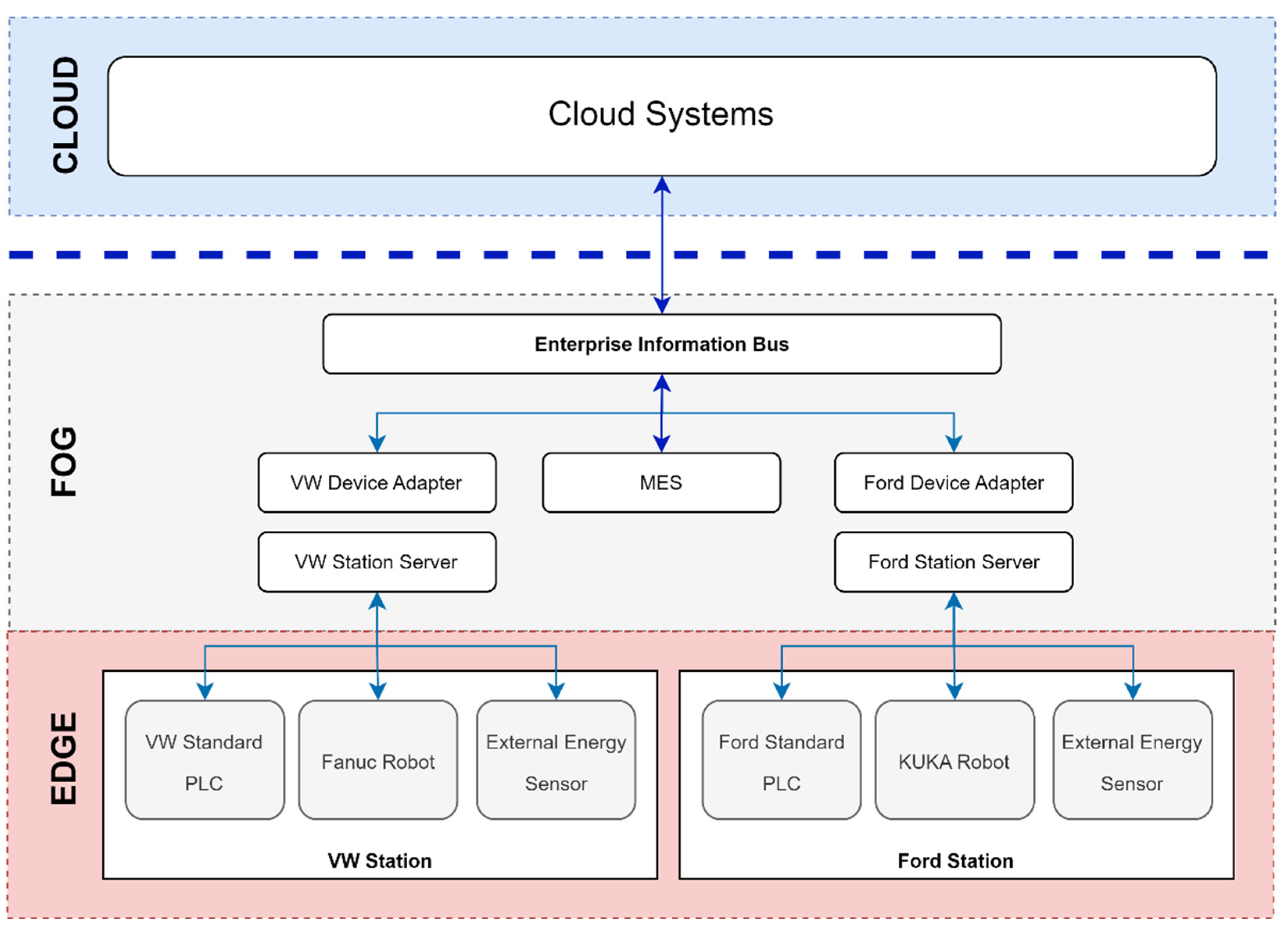
Furthermore, both cells integrate an orchestrator that follow Industry 4.0 ideologies, regarding the ability of devices to provide a free flow of information between the shop floor and cloud systems, such as the one proposed in this article. This orchestrator, shown in
Figure 4, is composed of four major components: (i) the Station Server, which is responsible for controlling unit production processes, named skills, and collecting raw sensor data from the equipment of a generic cell; (ii) the Device Adapter, which is responsible for controlling complex production processes, named recipes, and transform the raw sensor data obtained in the Station Server into relevant key performance indicators(KPIs); (iii) the Enterprise Information Bus, which is responsible for handling communications between the components, managing production orders and to provide interfaces that allow the transfer of data to outside systems; and finally, (iv) the MES, which is responsible for the distribution of products to be produced across the available stations in the system. This separation of responsibilities into several components allowed the orchestrator to be more agile and flexible, when confronted with different end user requirements, making it relevant to a wider array of possible implementations.
Regarding the use case at hand, the orchestrator provided was parameterized to: (i) allow production in both stations simultaneously, following rules in order to decrease station idle times; (ii) allow the production of two different products, using 5 (Weld) and 8 (Weld Complex) welding points, respectively; and (iii) report for each product produced the following KPIs: Duration, Consumption, Robot Consumption and Cell Consumption, verified in each skill and recipe executed. In addition, the communication protocol used between the internal components of the orchestrator was OPC-UA, since this is still one of the most widely accepted protocols in the industry, and to export the data to populate the various Execution Data Tables, in order to publish product, recipe and KPI execution information.
2.3. Deployment
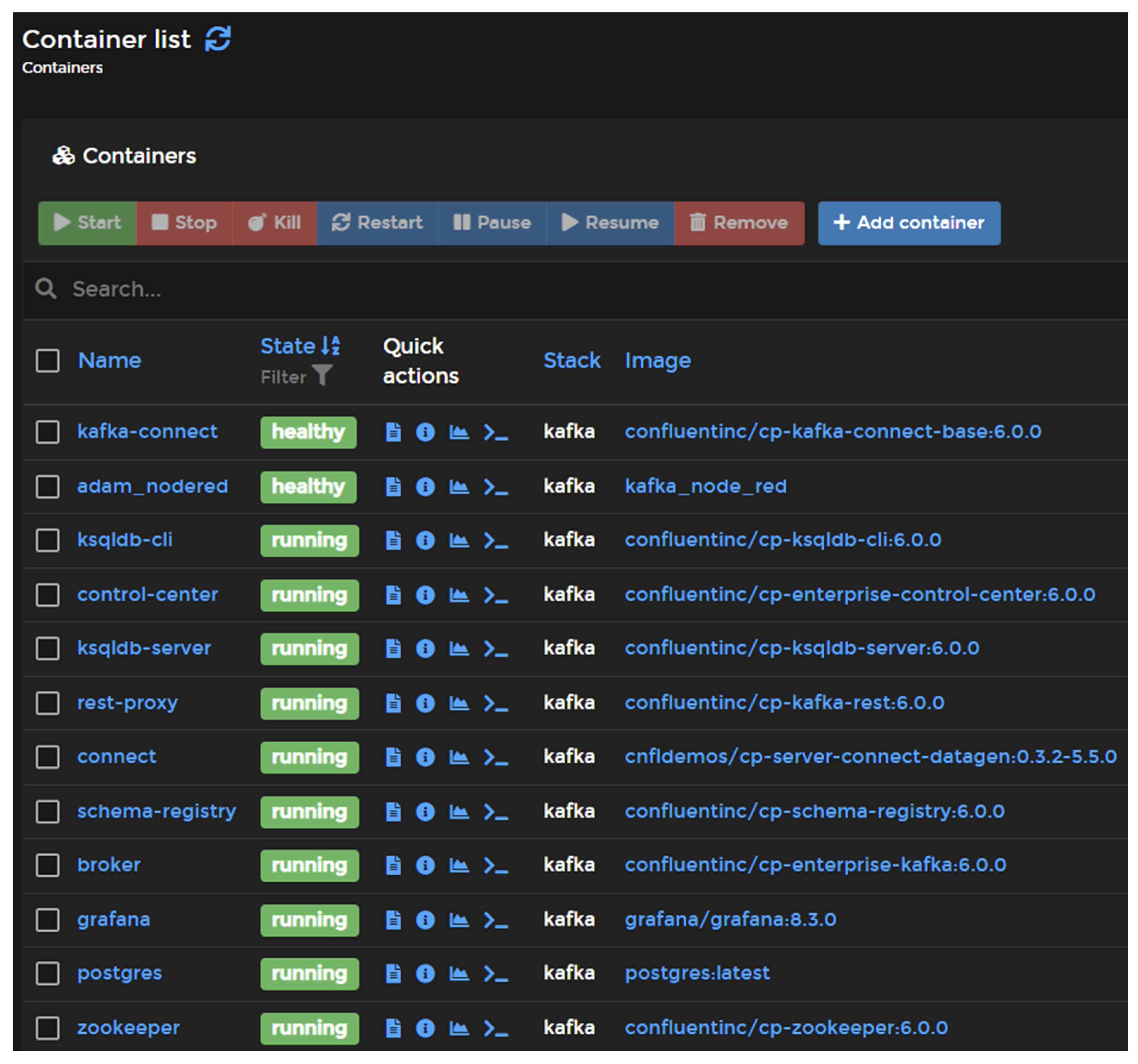
There are multiple ways to deploy software in the cloud, either by using several open software services, such as Cloud Foundry, or privately owned clouds, such as in the case of Google Cloud or Microsoft Azure. The most notable feature of most cloud-based software deployment platforms is their operation, as they typically use a container-based approach to deal with the deployed software. Thus, a privately owned server with a container-based approach can work very similarly to the core base of this software. As such, the portainer.io software was used to instantiate the system architecture. This software allows the user to easily deploy, configure and secure containers on Docker, Kubernetes, Swarm and Nomad in any cloud, datacenter or device.
Figure 5 depicts the Introsys server with the portrainer.io software, where several Docker containers are deployed. Each container can be described as a single program or system that is self-contained and can only communicate with other containers or with the outside in specific channels. The Docker software also has a repository with several programs built and ready to use, with the added advantage of being separated by version. This allows the same version to be deployed and maintained, facilitating the transitions from the test environment to the industrial sector or maintaining a compatible version that may break in later versions. Finally, the user’s own container can also be deployed, with a set of software and connections deemed useful for the situation and allowing the Docker software to build the container with the information and installation specified by the user. This was the specific case for the customized ML prediction software, which was then deployed in an API.
2.4. Machine Learning Predictive Models
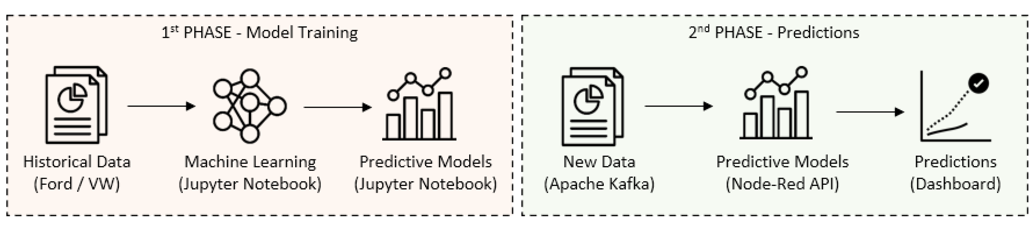
To train the ML predictive models that will be further deployed in the developed API (
Section 3.5), it is first necessary to collect the robotic cells sensor’s data that were subsequently sent by the middleware. These models were created using Python language and the software JupyterNotebook (
https://jupyter.org/, accessed on 5 December 2022).
Figure 6 shows the workflow diagram for the creation of the ML predictive models.
In the first phase (model training), data come from the Introsys facilities in a .csv format (historical data). These files were first pre-processed, in order to create the ML predictive models. Of the information coming from the robotics cells (Ford/VW), only a part was used for data analysis purposes, namely:
(a) Product Unique ID (product identifier);
(b) Product ID (name of the product);
(c) Recipe Unique ID (recipe identifier);
(d) Recipe ID (recipe type, it can be PWD—for Pick-Weld-Drop—or PWCD—for Pick-Weld Complex-Drop);
(e) Station ID (name of the station where the recipe was performed, i.e., Ford or VW);
(f) Velocity_* (robots’ velocity, in m/s);
(g) Duration_* (duration of respective task, in seconds);
(h) RobotConsumption_* (total robot energy for given task, in Watt-hour);
(i) Consumption_* (total cell energy for given task, in Watt).
The wildcard (*) stands for the three tasks of each recipe: “Pick”, “Weld/WeldComplex” and “Drop”. In cases where the parameters are just “Velocity”, “Duration”, “RobotConsumpion” and “Consumption”, it means that it is the sum of the three previous tasks, either “Pick”, “Weld/WeldComplex” or “Drop”. Four predictive ML models were created, two for each robotic cell and two for each type of recipe, as follows: (a) Ford_PWD; (b) Ford_PWCD, (c) VW_PWD and (d) VW_PWCD.
In the second phase (predictions), the new data (i.e., the recipes which are executed by the robotics cells) are sent through the middleware to the API (
Section 3.5) that contains the predictive models. These same recipes were used to predict: (a) the values of the execution duration of each recipe and/or task; (b) the energy consumption of each robot; and (c) the energy consumption of the respective robotic cells.
3. Results
Utilizing the robotic cells previously presented as well as the developed architecture, an implementation was made with the objective of extracting real-world results. After the integration of the robotic cells with the cloud-based middleware, in this case, Apache Kafka, the data collected after each process are both stored in a database (Postgres Database) and used for the prediction ML models regarding the ideal results of the energy consumption. The Node-Red API was built that uses the ML models and then store the predicted values in the database. Finally, an HMI made in Grafana uses the values from the database to make intuitive and simple-to-read graphs that represent some important metrics of the production process.
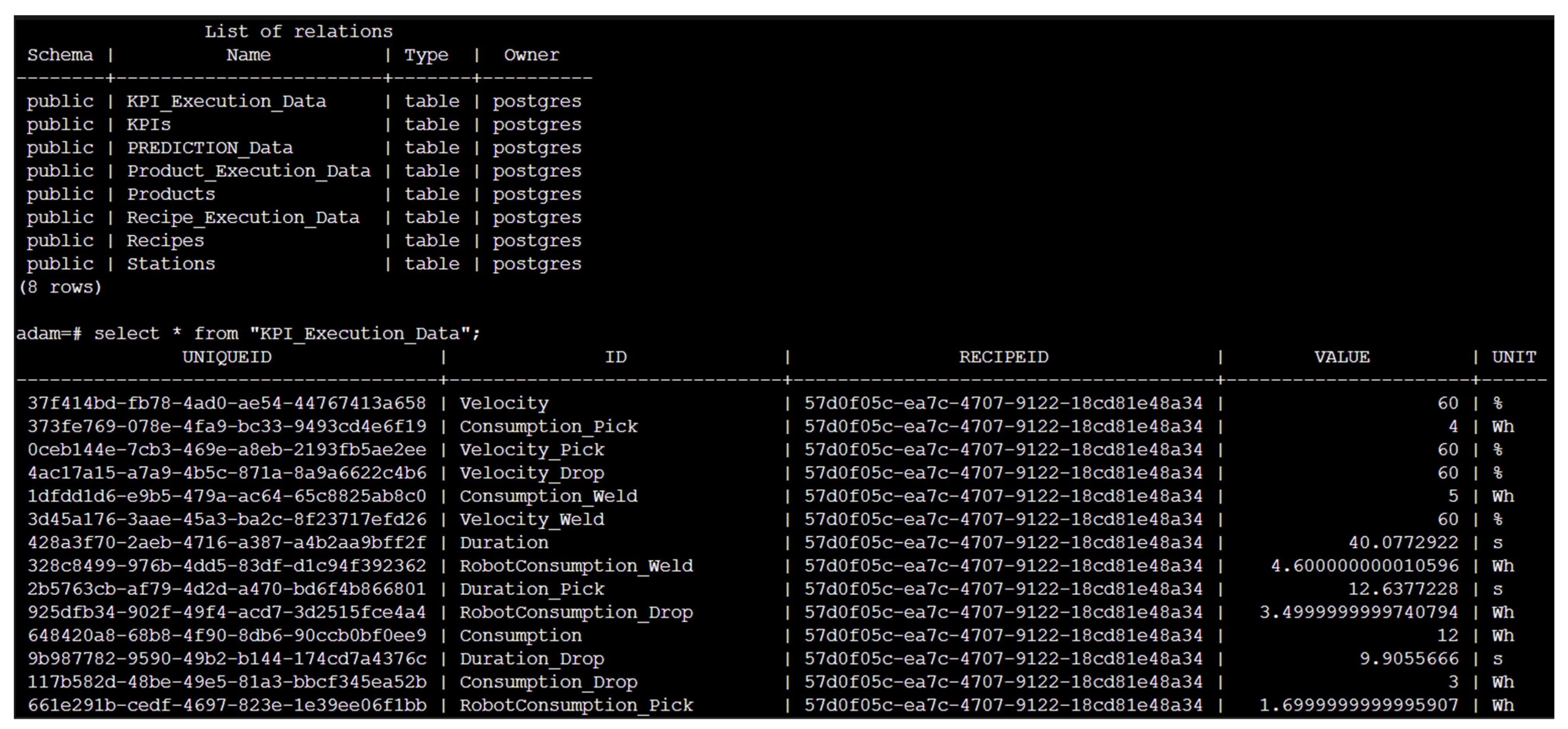
3.1. Data Model
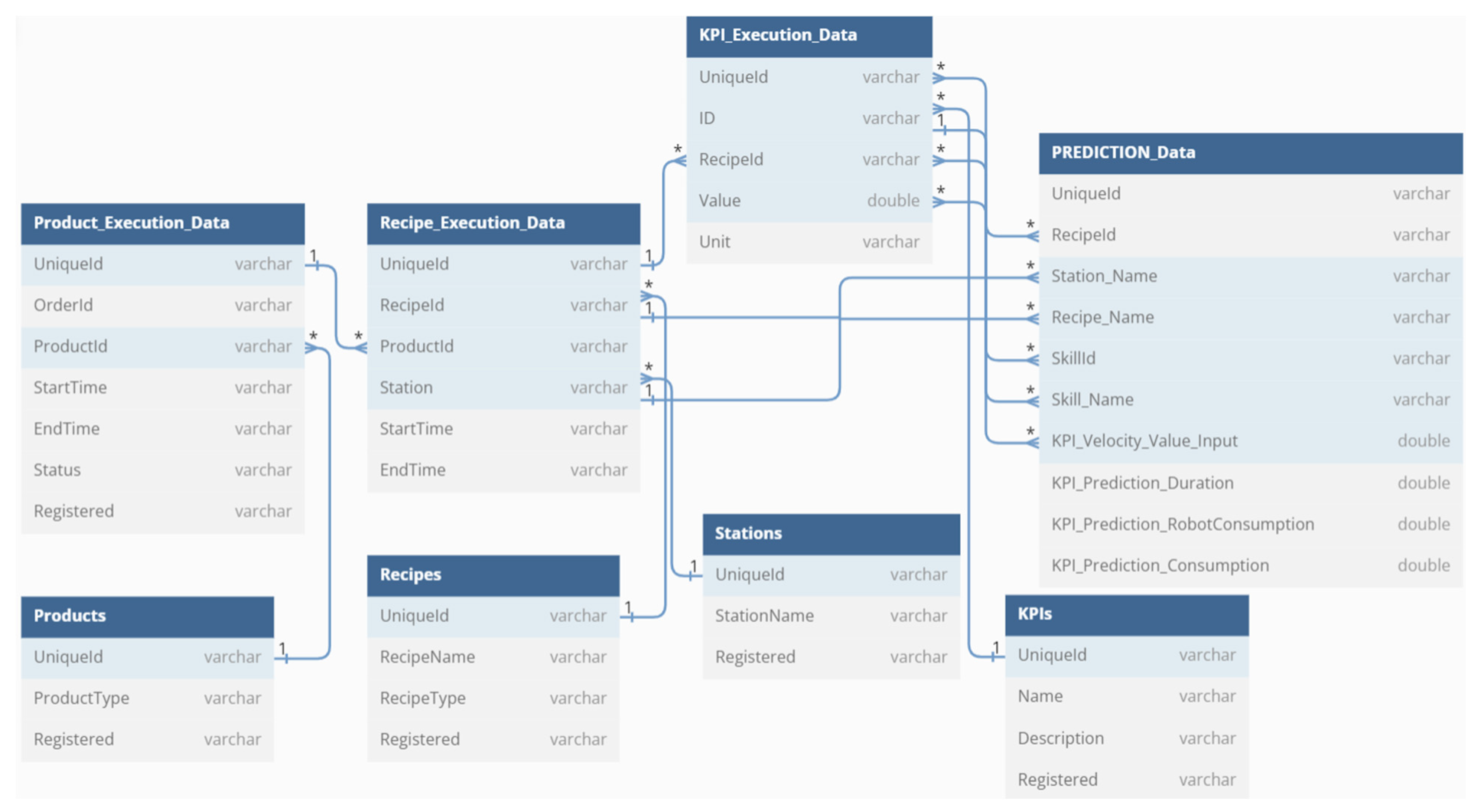
In
Figure 7, the data model of the implementation is presented. In this demonstration, eight tables were made, accommodating all the necessary and available data from the execution of recipes and products to the catalog of the different recipes, products and stations available in the factory. The prediction table stores the ML model’s prediction, connecting the existing execution data with that of each recipe as well as their key performance indicators (KPI), allowing to correlate the prediction of the models with the real values. The correlation can be further used to analyze some flaws that the machine might have, as it represents an excess of consumption in the models. It is also worth noting the relationship between each table, as it helps present a clear picture of the behind-the-scenes work of the data flow, not only in a real industrial environment but also in the specific case of this demonstration and ML model usage.
3.2. Flow of Data
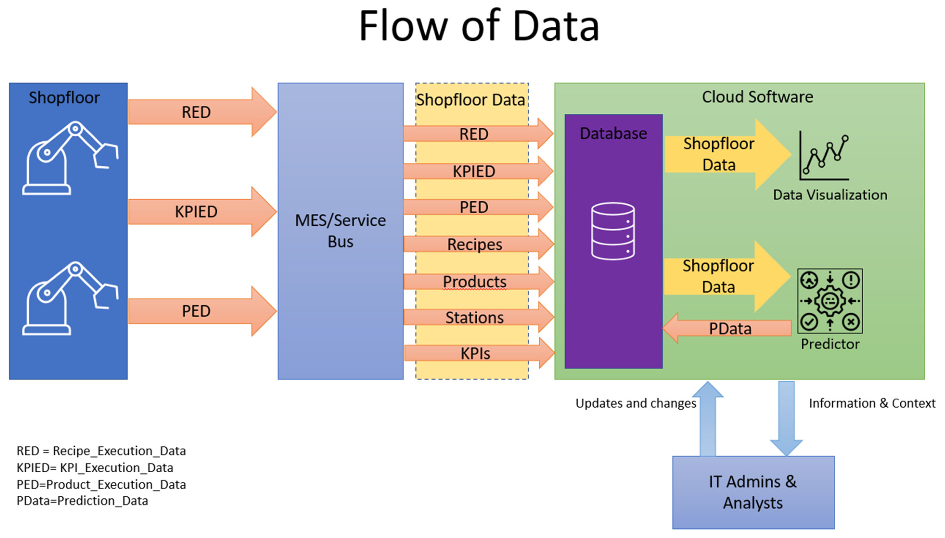
From the previously mention figure, it is possible to see the flow of data collected from the shopfloor, mainly the Recipe_Execution_Data, the Product_Execution_Data and the KPI_Execution_Data. This information is transmitted to the Introsys MES and Service Bus systems. These systems are also responsible to send and keep the information updated in the database regarding the Products, Recipes, Stations and KPIs. The Service Bus is then responsible to send to the database all the information previously mentioned; this information will from now on be called Shopfloor Data. The Shopfloor Data are now stored on the cloud database, each in their respective table, that are then utilized by other types of software, such as the data visualization software, responsible to make easy-to-read graphs and tables of data in real time. The prediction software also collects data from the database and uses these data as inputs for the already created models, allowing the output of several metrics that are sent to the database as the Prediction_Data.
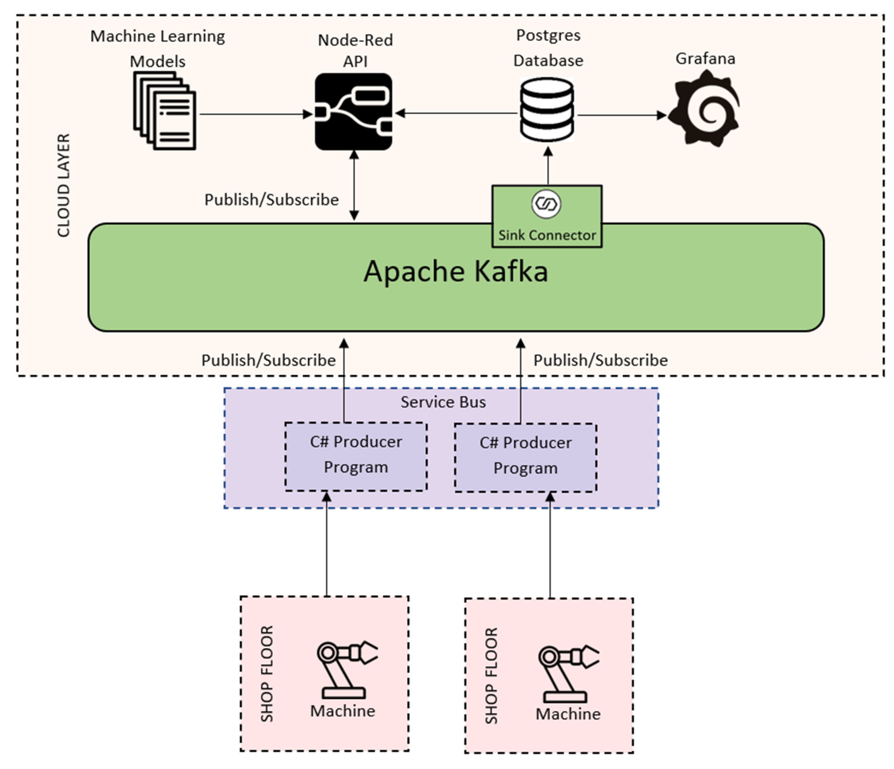
3.3. Implementation
The implementation of the architecture is presented in
Figure 9. This implementation comes from the necessity to send the information from the robotic cells, a cloud approach for data visualization, data storage (database) and data analysis services (in this case, using ML algorithms).
The implementation is made using two robotic cells that can make different types of recipes in order to complete a product. These robotic cells are connected to the Introsys service bus. The service bus, programmed in C#, is responsible for collecting the metrics from the robotic cells and agglomerating the information, such as the recipes and the products that are produced in the robotic cells. The service bus sends all the compiled data as JSON to the Apache Kafka middleware through the publish/subscribe approach using the C# available library. When the information is in Apache Kafka on the respective topic, the information is then passed from the JSON original format to AVRO, and finally, utilizing the Java database connectivity (JDBC), a stream is created connecting the Apache Kafka middleware to the Postgres Database, which is also deployed in the cloud. Lastly, it is important to talk about the Node-Red API, which contains all the ML models already trained and ready to be used. When new KPIs are sent to Apache Kafka, the Node-Red API receives a trigger (as it is subscribed to the topic) and collects useful information for the models using the PostgreSQL database. Finally, the Node-Red API processes these data and makes a prediction of duration, total consumption and robot consumption and registers this in the PostgreSQL database.
Message Broker
The middleware used in the implementation of the architecture was Apache Kafka. Apache Kafka is a message broker/streaming service that allows topics to be published and subscribed to by dedicated libraries and an API. Apache Kafka also excels in scalability, allowing it to serve as the architecture’s middleware with ease, connecting all shopfloor machinery and cloud applications. Moreover, Kafka enables the use of streaming services, connecting cloud applications, such as databases, through a stream without the need for an intermediate program and giving a constant flow of information as soon as it arrives at the topic. A more focused view of the message broker can be found in an article written by the team that addresses the middleware functionalities in greater detail, focusing on the message broker and why Apache Kafka was chosen [
27]
3.4. Machine Learning–Creating the Predictive Models
To create the four predictive models mentioned in
Section 2.4 (Ford_PWD, Ford_PWCD, VW_PWD and VW_PWCD), “Velocity_*” was considered as an independent variable (i.e., input) and “Duration_*”, “RobotConsumption_*” and “Consumption_*” as dependent variables (i.e., outputs).
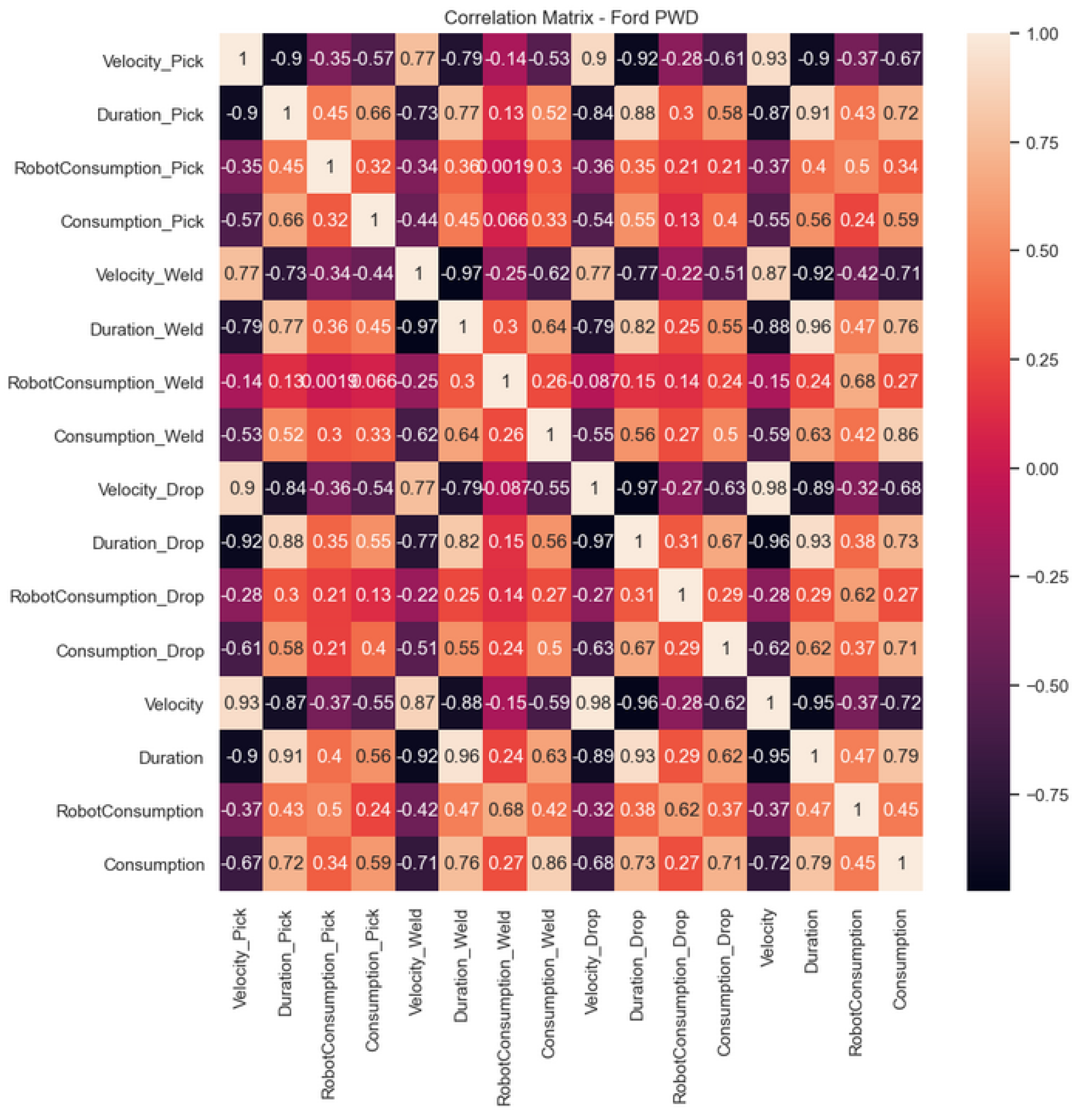
Figure 10 presents the correlation the connection matrix resulting from these parameters for the Ford_PWD predictive model. The same analysis was carried out for the remaining models.
Two ML regression models were trained with the intention of creating the desired energy profiles: Linear Regression and Random Forest. Linear Regression was used as a baseline and Random Forest was chosen since it represents a general-purpose ensemble approach (multiple decision trees), which is generally more robust, less prone to overfitting and can handle larger datasets more efficiently, often being used in the literature for predicting energy consumption [
21]. The tradeoff in this case is that it may require more computational power and resources; however, this was not a constraint for the use case at hand.
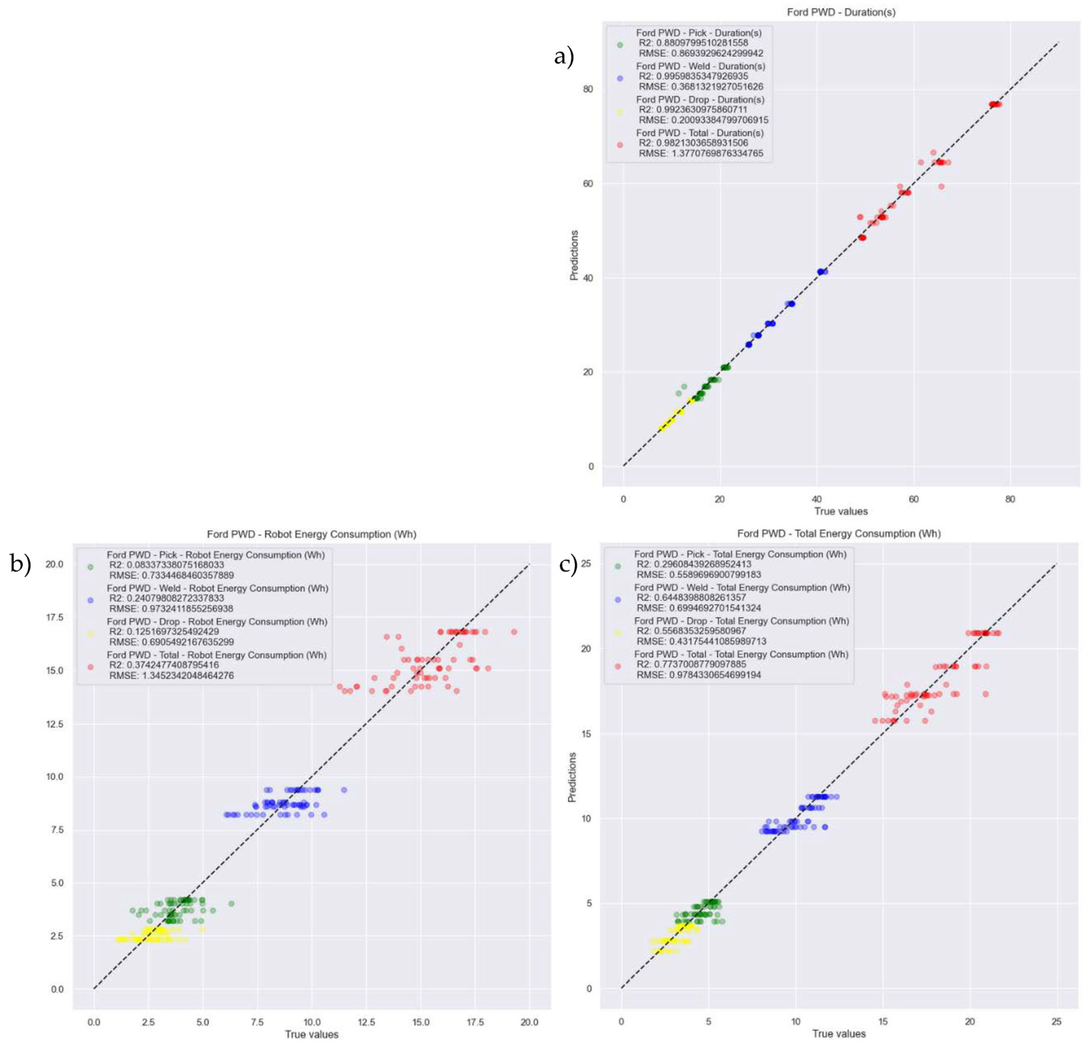
Table 1 presents the R-squared (R
2) and Root-mean-square error (RMSE) metrics as these two metrics are used to calculate the evaluation of the four predictive models. The random forest regression algorithm was used to create these models, and according to [
28], R
2 and RMSE are the most used metrics for evaluating regression models.
As is possible to see from
Table 1, the Duration parameter provides the best results, both for the R
2 and RMSE metrics, in the four models. This was expected, since the Duration is controlled internally by the orchestrator, and is not dependent on hardware devices (i.e., sensors) installed in the Ford/VW cells. The robot energy consumption (RobotC), however, provide the worst results, since these are dependent on the accuracy and quality of the hardware devices. The same happens with the total energy consumption (TotalC) parameter. This has a direct impact on the effectiveness of the predictive ML models, and consequently, on the comparisons between the predicted and actual values recorded.
Figure 11 illustrates the predictions (y) versus real values (X) and R
2 and RMSE metrics for the predictive model Ford_PWD. The same logic was used for the other models.
3.5. Creating the Node-Red API
An API using Node-Red was created to support the communication between the Apache Kafka and the predictive ML models. This API is based on the Publish-Subscribe principle and contains additional palettes for the API to work as desired, namely “node-red-contrib-kafka-client”, “node-red-contrib-queue-gate”, “node-red-contrib-machine-learning-v2” and “node-red-contrib-postgresql”.
The developed API contains several flows and nodes to work properly. However, this paper addresses only the most relevant steps, namely the communication with the Apache Kafka and the nodes that contains the ML predictive models. As such, six steps were identified:
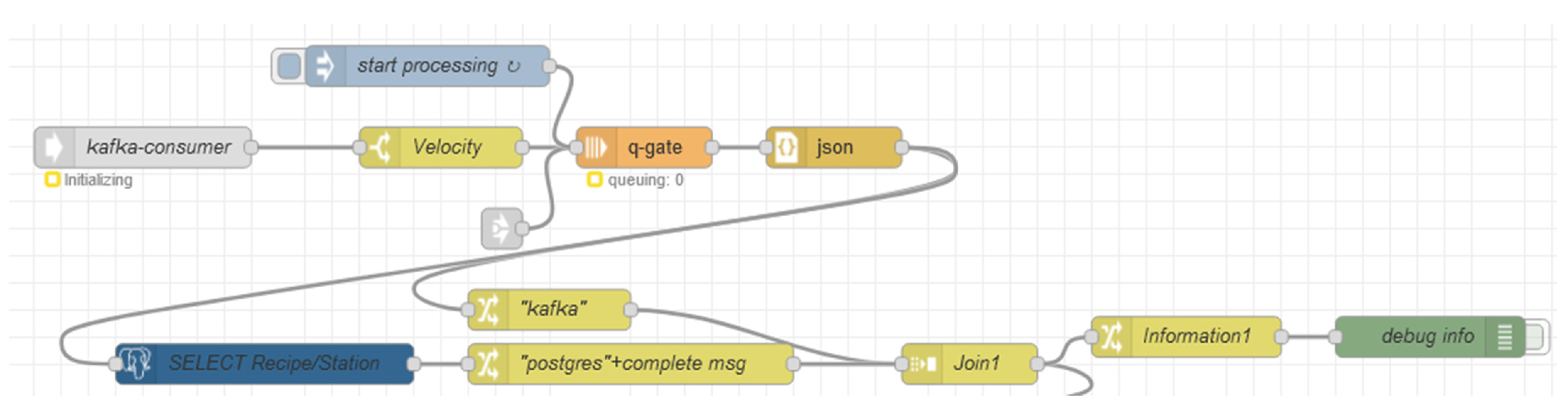
Step 1: Communicating with Apache Kafka: The first step was to trigger the information from the Apache Kafka. The node “kafka-consumer” was created (
Figure 12), so it was able to configure the Broker, Host (broker: 29092) and Topic (KPIEDTest).
Step 2: Filtering messages containing “Velocity”: The second step was to filter the messages coming from the “kafka-consumer”. As mentioned in
Section 3.4, the parameter “Velocity_*” was considered the independent variable, and as such, it was used as the input of our API. The switch node “Velocity” (
Figure 12) was used to filter the messages that contains the string “Velocity”.
Step 3: Selecting the RecipeID and StationID: A postgresql node “SELECT Recipe/Station” was created (
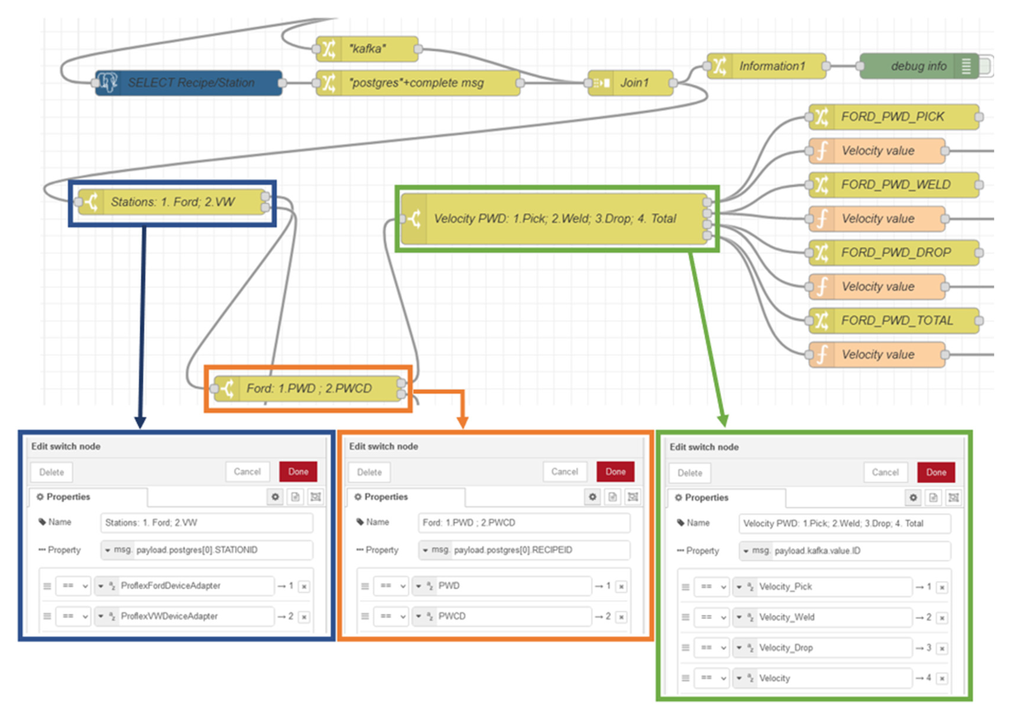
Figure 12) in order to select the RecipeID and StationID from the PostgreSQL database. It was necessary to configure the server and develop a query. Additionally, two change nodes were created ““kafka”” and ““postgres” + complete msg” to store the information desired from Apache Kafka and the PostgreSQL database, respectively. This information was posteriorly joined and stored in a change node “Information1”.
Step 4: Routing the messages: We started the fourth step by filtering the Stations (i.e., Ford or VW), using the switch node to route the messages based on sequential position. Using the same logic, two new switch nodes were created, one for the Ford station (Ford: 1. PWD; 2. PWCD) and another for the VW station (VW: 1. PWD; 2. PWCD), where it is possible to filter the type of Recipe (PWD or PWCD).
Figure 13 illustrates the flow and configuration of the mentioned nodes.
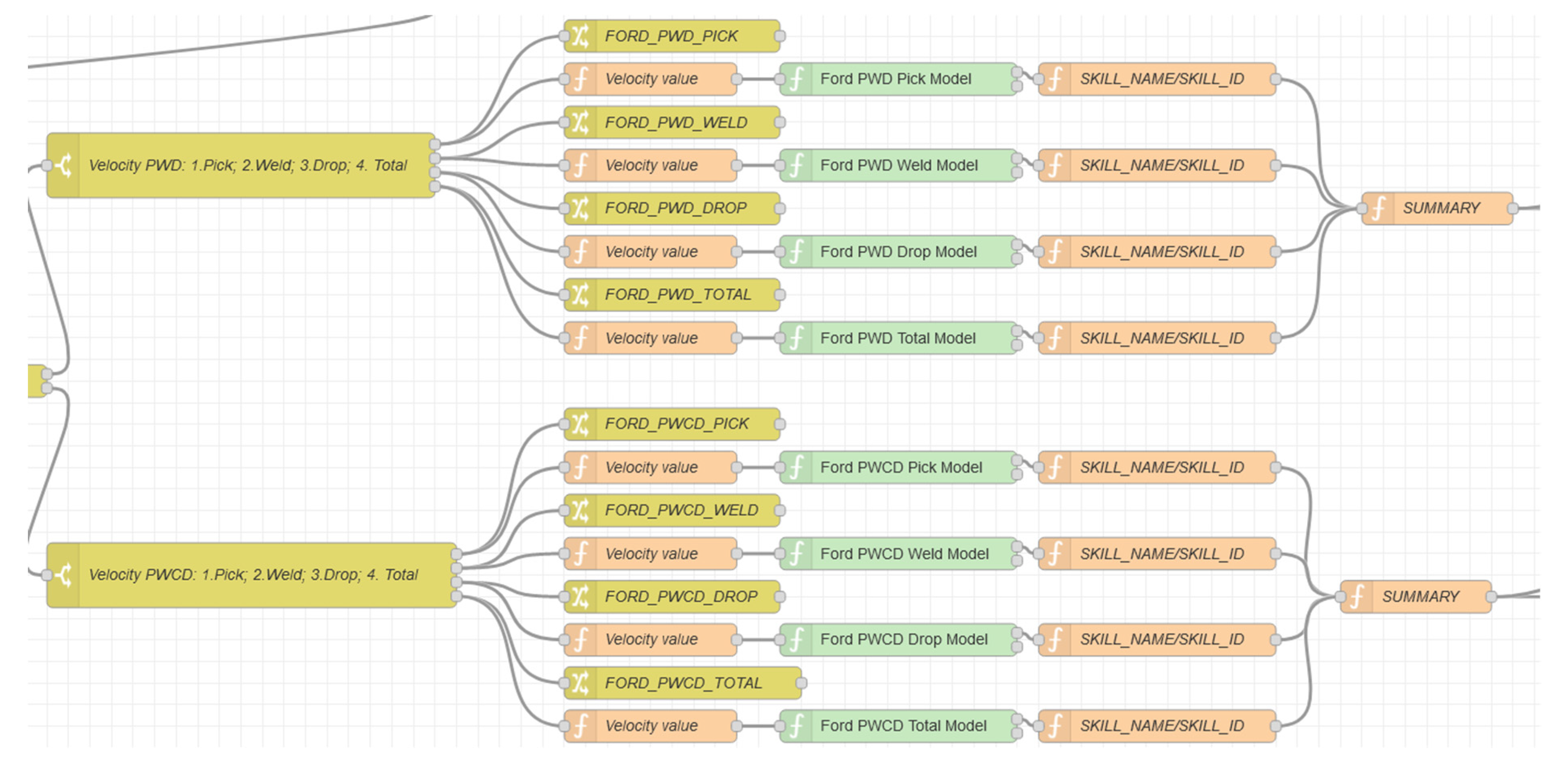
Step 5: Deploying the ML predictive models: After creating the route for the messages, it was time to deploy the ML predictive models. Thus, sixteen nodes were created, each one corresponds to a respective task (Pick, Weld/WeldComplex, Drop), of a respective recipe (PWD and PWCD) and of a respective station (Ford and VW).
Figure 14 shows the ML predictive models (green nodes) for Ford station. The same logic was used for VW station.
As explained in
Section 3.4, “Velocity_*” was considered as an independent variable and “Duration_*”, “RobotConsumption_*” and “Consumption_*” as dependent variables for the ML predictive models. Therefore, the input of the ML predictive model nodes is the value of Velocity (four values for each task), and as an output, the models give the values of Duration, RobotConsumption and Consumption.
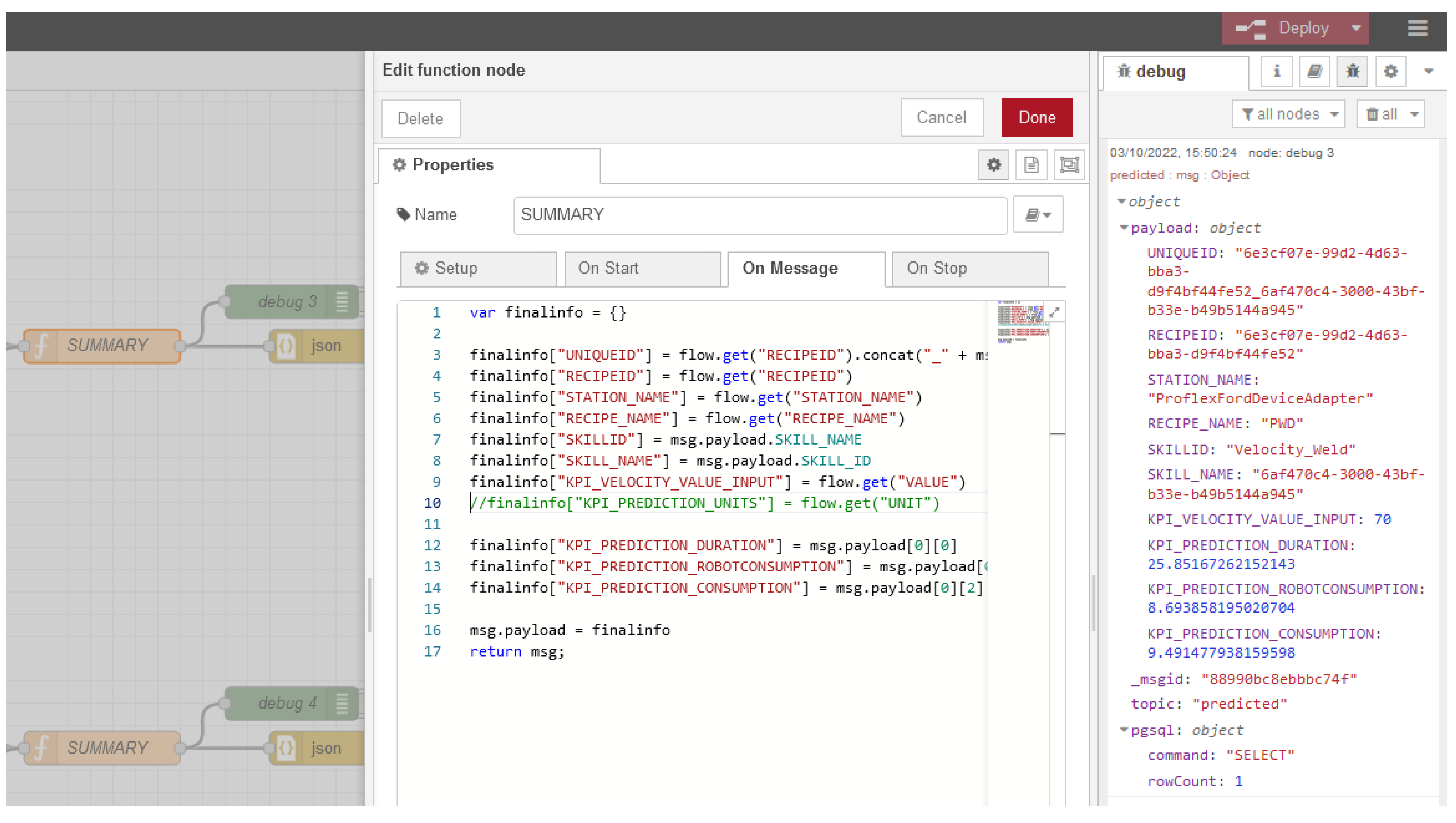
After the ML predictive model nodes, the function node “SUMMARY” was created to track and store all the information that is needed (
Figure 15).
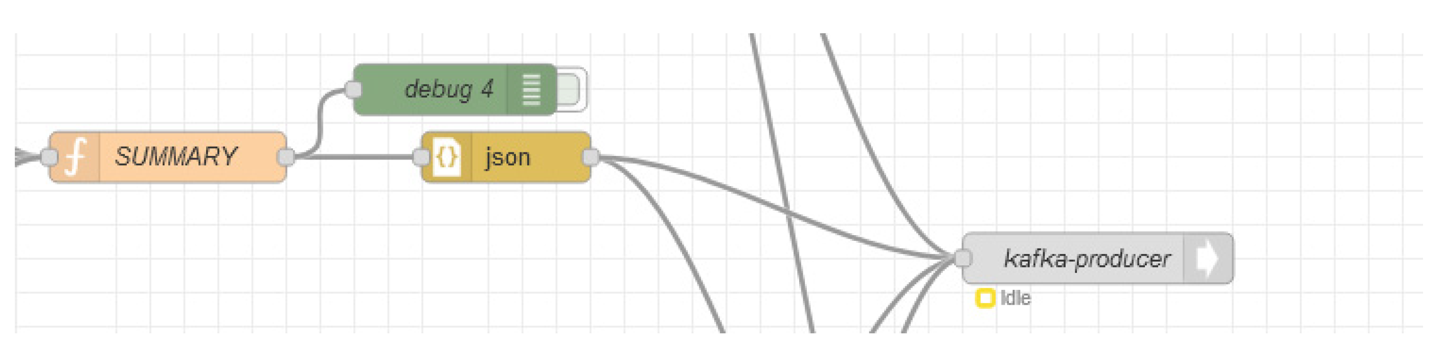
Step 6: Sending the information to Apache Kafka: Finally, and similarly to what was done with the “kafka-consumer” node (
Figure 12), a new node, “kafka-producer”, was created (
Figure 16) and configured in order to send the information back to Apache Kafka, with the difference of the Topic, untimely creating a new table in the database with the prediction results named “PREDICTIONTest”.
3.6. Data Visualization
Despite all the relevant information being stored in the PostgresSQL database, the reading of this information for a human being is not an easy task. It is important to quickly assess some metrics and check the correlation between values, to be assured that all the processes are working properly. The PostgreSQL database is depicted in
Figure 17, along with a specific table with some values. It directly correlates with the data model in
Figure 7, as it is the main database and the one used to store all data for visualization and tests. It is easy to prove by this demonstration that some metrics are hard to correlate like this and visualize, and when more metrics start to integrate in the correlation of tables, it becomes clear that this is not a good way to display information.
To display all this information in a more useful and human-friendly way, the Grafana software was used. Grafana allows the use of SQL queries to make time graphs, histograms, display tables and even create alerts in case of something going past specific values. In the specific case of this demonstration, the graphical interface is alternated and separate for each one of the robotic cells in order to facilitate and separate the analysis of each one. The prediction analysis is also demonstrated here. There is some discrepancy regarding some values, as they are based on some simulated values that do not represent the real metrics. These simulations were made by the company Introsys to test some systems. Nevertheless, it is possible to see the different recipes and consumption patterns and compare them with the predictive value, allowing the detection of problems and irregularities without the need for any more systems.
From top to bottom, it is possible to see on the dashboard:
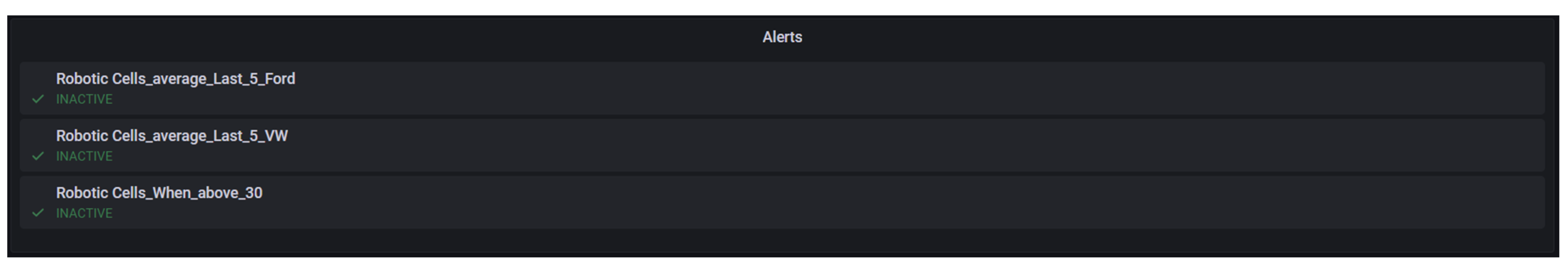
Alerts: In
Figure 18, three alerts were created, with the objective of alerting the user if some basic metrics were out of control. The first two alerts are equal but for different robotic cells, and they measure the last entry and compare it with the average of the last five entries. If the value is superior to 15% of the average value, the alert is raised. The final alert checks if the last entry is bigger than 30 Wh and raises an alert if it is.
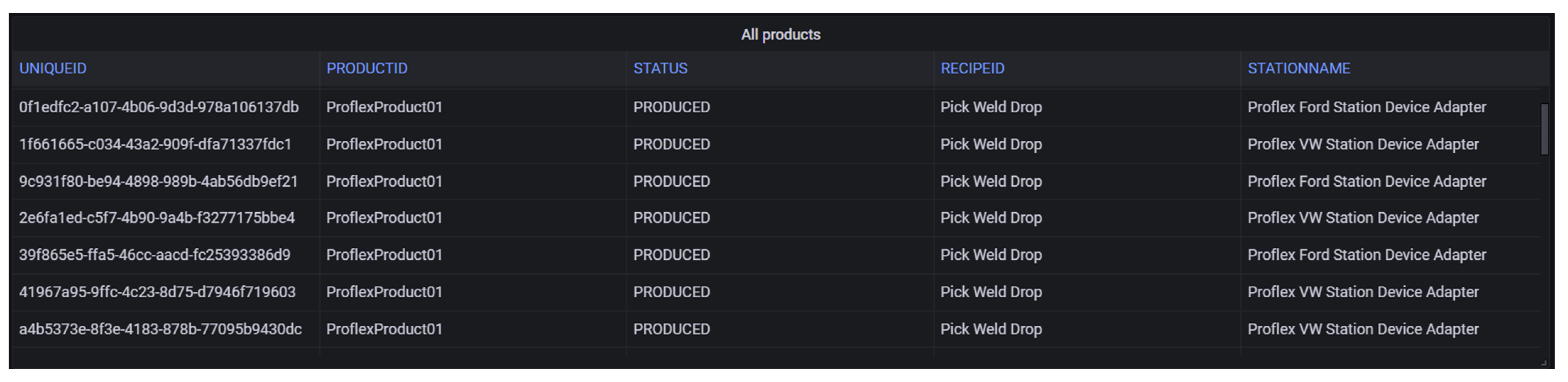
Products: In
Figure 19 is a simple table that shows the products of the factory and their status, ordered by the “not produced” products.
Figure 19.
Products panel.
Figure 19.
Products panel.
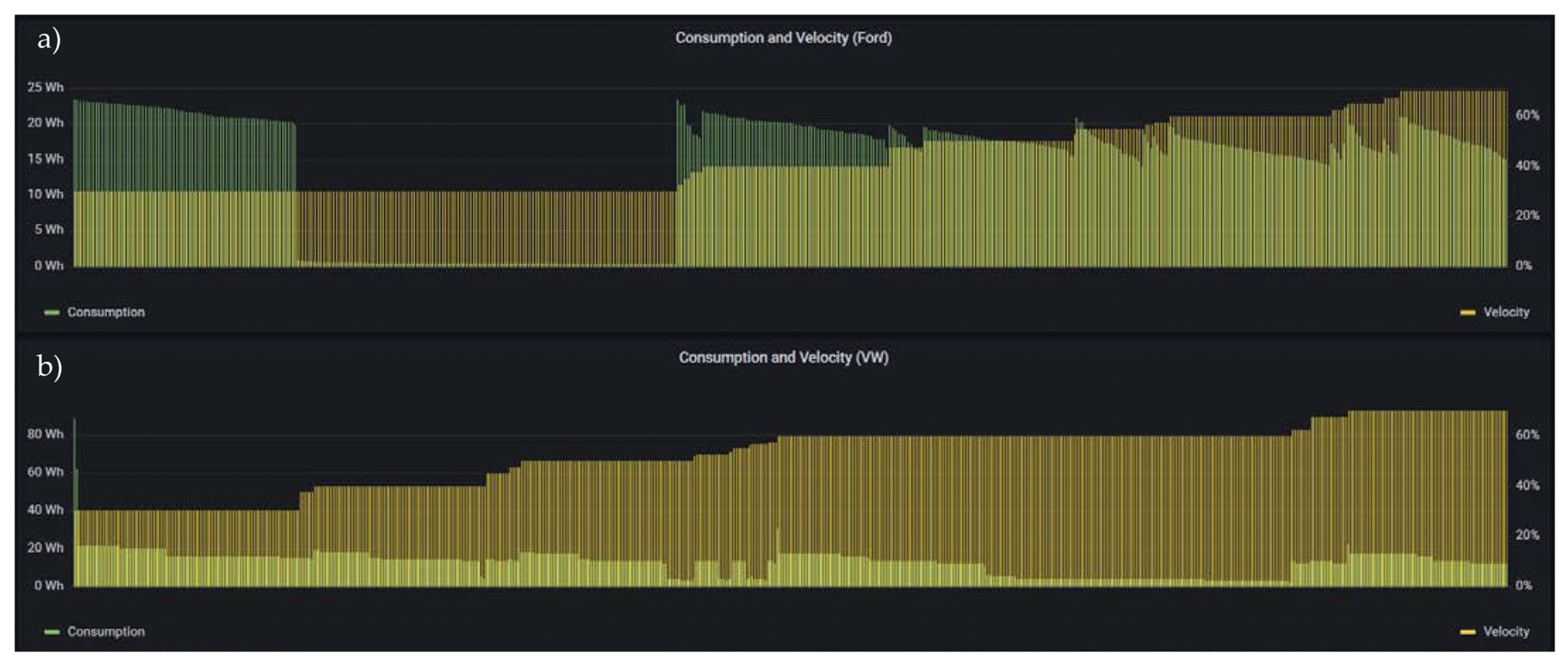
Consumption/velocity: In
Figure 20, there are two similar bar charts, one for each robotic cell. These bar charts represent the energy consumption paired with the velocity as a percentage. This metric allows the worker to quickly check if something is going wrong with the robotic cell. In this figure, it is possible to see some values where the energy consumption is very low, as it represents some simulations made by Introsys with non-representative values.
Figure 20.
Consumption/Velocity Panel (a) for the Ford robotic cell and (b) for the VW robotic cell.
Figure 20.
Consumption/Velocity Panel (a) for the Ford robotic cell and (b) for the VW robotic cell.
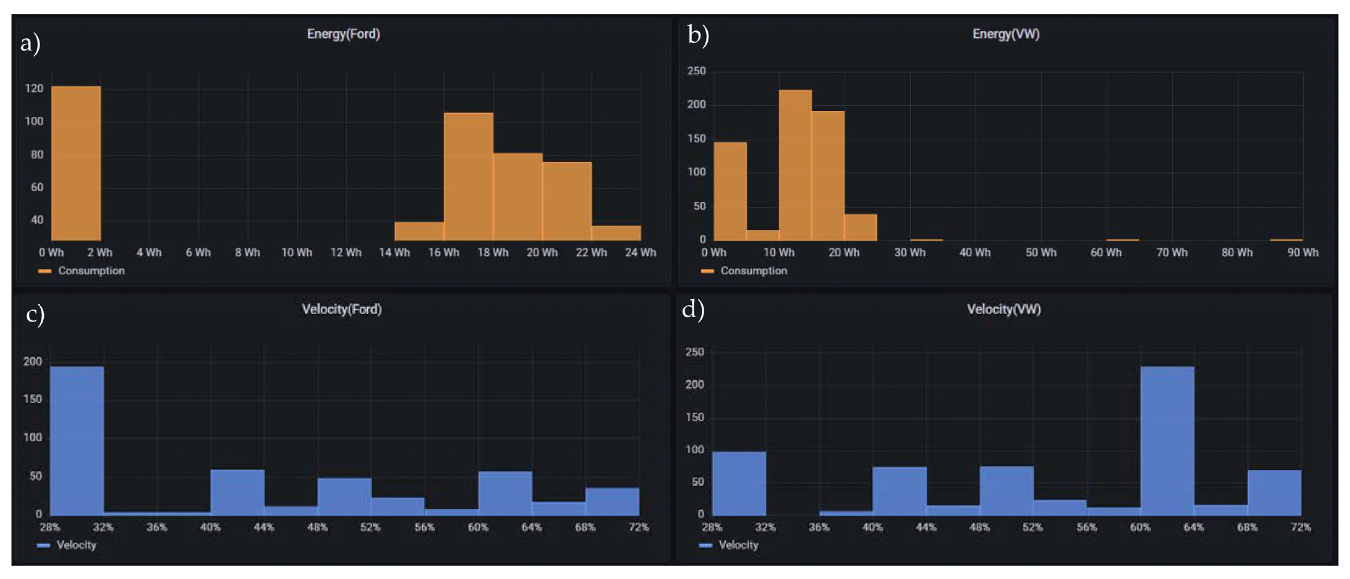
Energy/Velocity histogram: In
Figure 21, there are two similar histograms, one for each robotic cell. These histograms represent the energy consumption and velocity of each robotic cell. Histograms (a) and (b) represent the number of times of each the energy consumption intervals of the robotic cells from Ford and VW, respectively, while histograms (c) and (d) represent de number of times of the velocity intervals, also of the Ford and VW robotic cells, respectively.
Figure 21.
Energy/Velocity histogram panel, the (a,b) the energy consumption for Ford and VW respectively and the (c,d) the percentage velocity for Ford and VW respectively.
Figure 21.
Energy/Velocity histogram panel, the (a,b) the energy consumption for Ford and VW respectively and the (c,d) the percentage velocity for Ford and VW respectively.
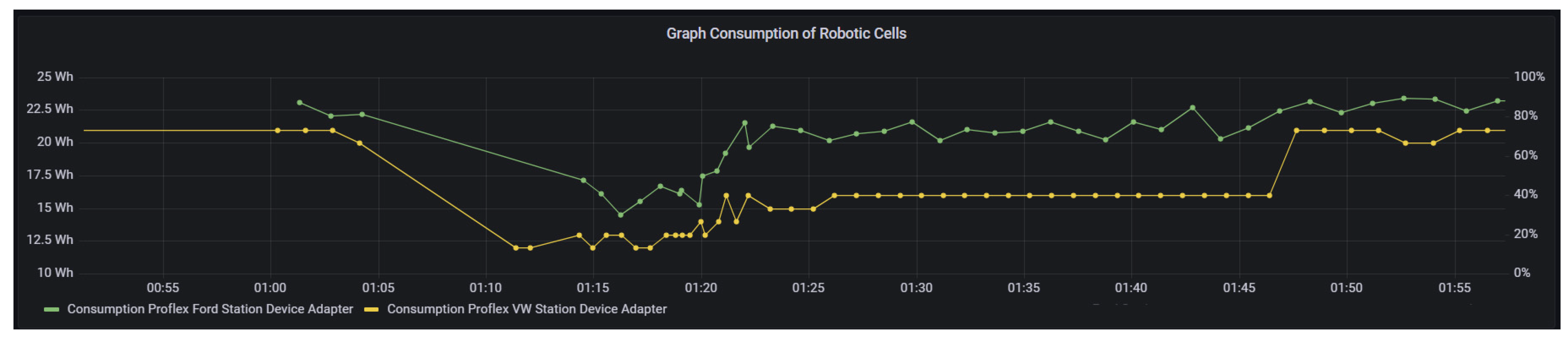
Time graph of robotic cell consumption: In
Figure 22, the time graph is a junction of four different graphs that the user can choose and even correlate with different metrics. The worker might want to see the consumption and velocity, or the consumption of both robotic cells, and this graph allows that customization.
Figure 22.
Time graph of each robotic cell energy consumption.
Figure 22.
Time graph of each robotic cell energy consumption.
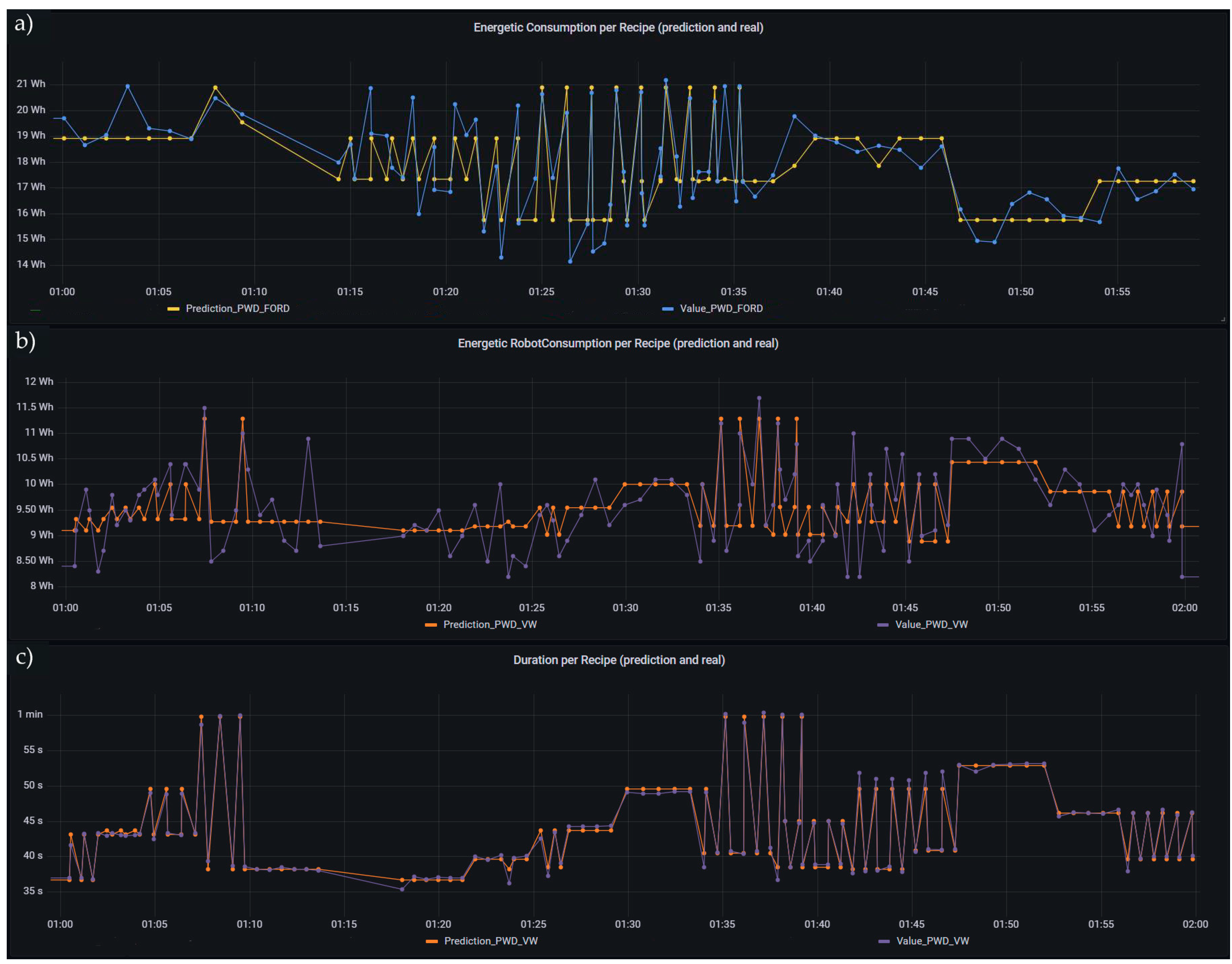
Predicted and real values per recipe: In
Figure 23, these graphs allow the user to choose different metrics and correlate them between the different recipes and stations with the predicted and real values of (a) cell, (b) robot energy consumption and (c) duration. This graph is deemed extremely useful, as it can show the total consumption or duration of the different robotic cells and compare them in an easy-to-read value with the prediction values. This allows the worker to easily check which station is having problems or is performing in a way that is out of the ordinary.
4. Discussion
The study conducted by the authors represents a vertical use case from shopfloor to cloud of a real implementation of cloud-based applications used by robotic cells that complies with Ford and VW production standards. From this study, it is possible to see a cloud application cable that can be used by any machine or software as long as it is connected to the middleware [
27].
In Industry 4.0, the deployment of a cloud-based application software allows an increase in efficiency of resources (for example, programs can be instantiated in the cloud and not locally), allowing easy scalability and integration from different shopfloor machines, but also from other software or even workers. Moreover, the centralization and sharing of such processes can easily allow the comparison and scheduling of production based on the results of the data gathered and processed by the software.
In this study’s specific case, the use of prediction software allows the understanding of which processes, recipes and products are more efficiently produced in each robotic cell. The scheduling of production should be done by considering the energy consumption of each process and efficiently produce each product. Another use of this prediction of energy consumption is the possibility of detecting any inefficiency or problems with the machine sooner than with other methods. Some problems could be detected if the energy consumption of the machine starts to increase in relation to the prediction, such as in the case of lack of lubrification or any problem contributing to the excessive effort of the motors to achieve the same production.
It is also critical to recognize some important aspects of this study. First, the test was conducted using only two robotic cells, and although the middleware and cloud-based software were ready to handle an increasing number of communications, restrictions in terms of hardware disallowed it, as no more robotic cells were available to be utilized in the study. Second, regarding the prediction results provided (
Table 1) it is clear that KPI Duration provides better results, and this was expected since the KPI Duration is internally controlled by the orchestrator, resulting in a KPI independent from all hardware devices installed in the cells. On the one hand, KPI Consumption in VW and KPI Robot Consumption in Ford provide the worst results in terms of differences between the predicted and actual registered value, and this was also expected, since it introduces dependencies on hardware devices. In the case of the KPI Consumption of VW, the sensor used provides energy consumption with some level of uncertainty due to its magnitude, which can result in an innate error that can reach ±10% of the normal detected values. This has a direct influence on the training of the ML model, and consequently, on the comparisons between the predicted and real values registered. On the other hand, the KPI Robot Consumption in Ford uses a sensor that monitors tri phase powers, which means that in order to obtain a consumption (energy), internally, the orchestrator is required to convert power to energy, and in consequence, make this process extremely dependent on sensor latency and update frequency. Since the provided sensor only allows low frequency values, this means that the energy calculated can incur significant variations in its reading from product to product. Regarding the chosen ML algorithm (Random Forest), it proved to be fast to train, easy to use, flexible, robust to noise and quite effective with prediction results very close to the real results (at least for the Duration parameter). This was expected, since, according to the literature, this model is very effective with regression problems and often used in predictive functions [
29,
30,
31].
Finally, is important to regard this study as an implementation test case, where the company had a specific problem that needed a resolution. The study was not meant to benchmark different approaches regarding ML algorithms, and as such, makes it difficult to compare to different studies (such [
22,
25]), as they do not deal with the specific cases and data of the present demonstration. Nevertheless, several studies relevant for this paper are mentioned in
Section 1.2; additionally, some important references for the creation and validation of the ML models are referenced in
Section 3.4.
As for future directions, the creation and use of an optimizer or scheduling software capable of automatically allocating the production based on time, cost efficiency or the best of both, by making the production the most cost-efficient at the given time, can be developed. Given that the scheduling is usually done manually, software that can take the inputs of the predictor software and compute the best-case scenario would be a great asset and an engineering feat.
5. Conclusions
This case study uses data from two shopfloor robotic cells that are on par with Volkswagen and Ford production standards to construct a ML algorithm capable of predicting the energy consumption of a product, based on the recipe and velocity of the process, and deploy these models on a cloud-based software API. Moreover, an HMI is developed capable to easy-to-read and adaptable graphs to facilitate the reading of important information and status either by a shopfloor worker or by a manager. This is based on an architecture capable of working with an expanding shopfloor’s machinery or software (both in the cloud and on the shopfloor), allowing an addition of the several layers of the factory. The work shows promising results, allowing for the prediction of the results of the energy consumption of each product with high accuracy, even with some measurement inconsistencies from the used hardware.
Nevertheless, is important to highlight some limitations of this case study, mainly the test of the architecture, which has only been implemented in a single factory, as it is important to use it in several different types of factories to be validated. Another important limitation is the data used for the models, which need to be collected when the machines are in prime state, as the condition of these machines will reveal a natural limitation of the models and consequently for all the predictions made since the model’s training. Finally, the limitation of input parameters as the only input parameters are the velocity and recipe type, so the models make the correlation between only these two parameters to compute an energy consumption.
It is important, in the future, to test the work done with several machines and products in a more complex environment. A scheduling software can be realized that can utilize the work done in this paper, mainly the architecture and the predictor software, to automatically schedule the machinery with different input parameters, for example, time, energy consumption and workers, and compute an optimal production schedule and machinery input for the given parameters.

 ,
, 


