
Numerical Simulation of the Operating Conditions for the Reduction of Iron Ore Powder in a Fluidized Bed Based on the CPFD Method
Abstract
:1. Introduction
2. Experimental Steps and Protocols
3. Mathematical Models
3.1. Governing Equations
3.2. Chemical Reactions
3.3. Simulated Experimental Conditions
4. Conclusion and Analysis
4.1. Metallization Rate
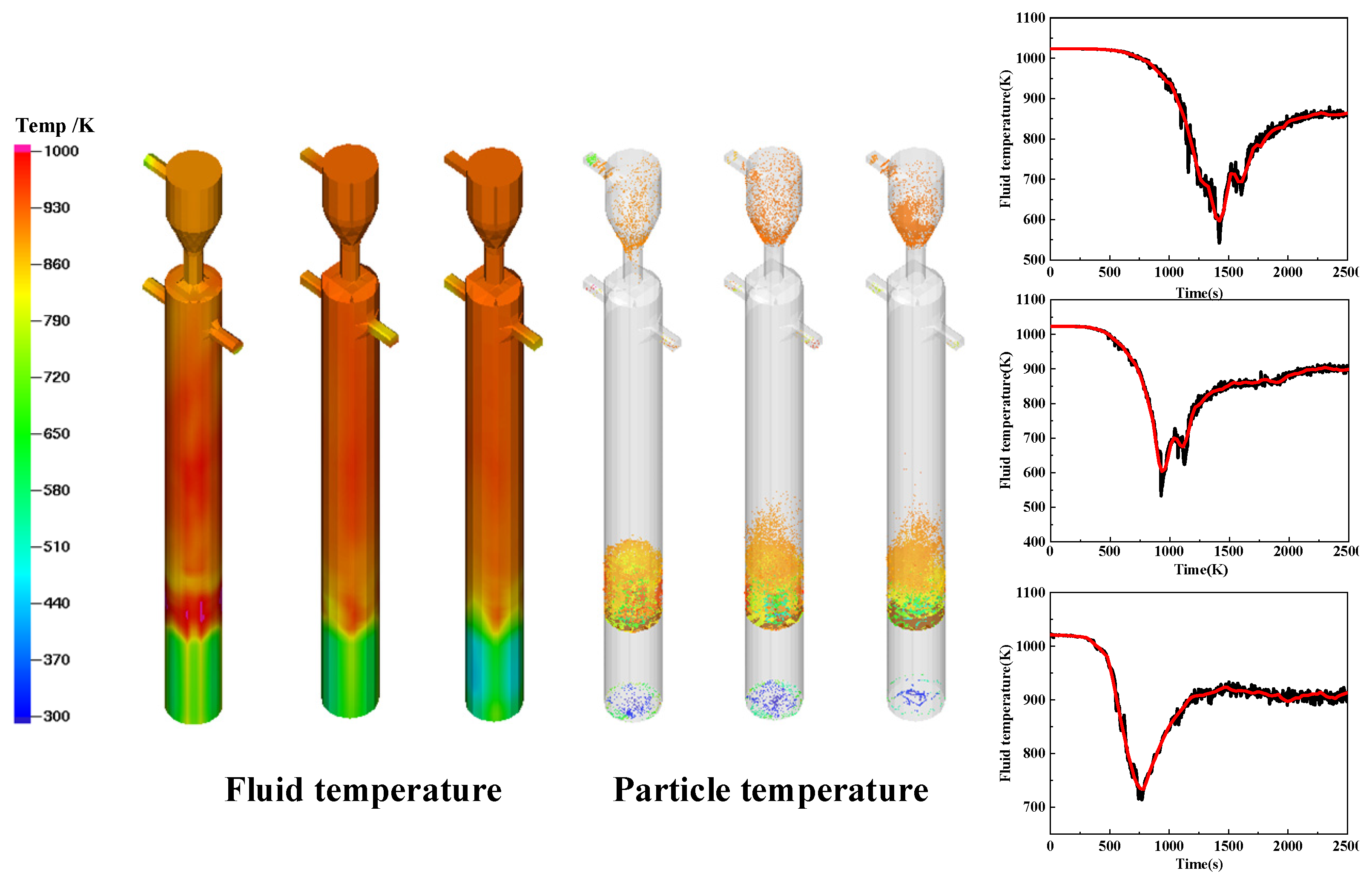
4.2. Reduction Temperature
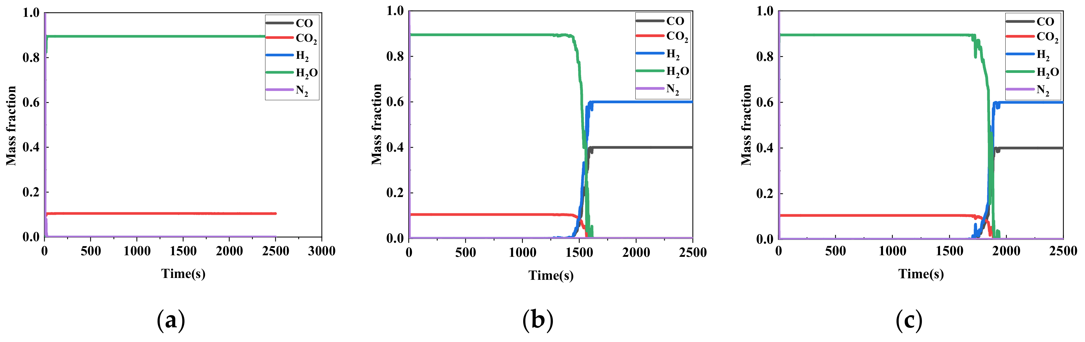
4.3. Types of Reducing Gases
4.4. Reduction Pressure
4.5. Linear Gas Velocity
5. Conclusions
Author Contributions
Funding
Conflicts of Interest
Nomenclature
| a | Pre-exponential factor |
| A | Particle acceleration |
| αg,αs | Gas and solid phase volume fraction |
| Cv | Specific heat capacity |
| Particle size, m | |
| Dg | Gas phase turbulent diffusion coefficient |
| Ea | Apparent activation energy |
| F | Force source, N |
| Fs | Frictional stress between particles |
| g | Gravitational acceleration, m/s2 |
| Local fluid wall heat transfer coefficient | |
| Dilute transfer heat coefficient | |
| hg | Enthalpy of mixture |
| Thermal conductivity of a fluid | |
| k | Rate constant |
| L | Bubble hole length, m |
| m | Particle mass, kg |
| δm˙g,i | Mass change of gas component i produced by homogeneous reaction |
| δm˙s | Change in gas mass per unit volume, kg/m3 |
| δm˙s,i | Mass transfer of gas component i from a heterogeneous reaction |
| ρg,ρs | Gas and solid phase density, kg/m3 |
| P | Average pressure, Pa |
| Prandtl number | |
| q | Energy transfer between gas phase and solid phase |
| q˙D | Energy changes due to component diffusion |
| Heat of reaction, J | |
| Qij | Thermal conductivity between particles |
| Qradi | Radiation heat transfer between particles and walls |
| Qreac | Heat of reaction |
| Qsg | Convective heat transfer between particles and gases |
| R | Molar gas constant |
| Re | Reynolds number |
| Sh | Energy transfer between gas phase and solid phase |
| T | Thermodynamic temperature |
| VP | Particle volume, m3 |
| ug,us | Gas and solid phase velocity, m/s |
| Yg,i | Mass fraction of gas components |
| τg | Gas phase stress tensor |
| τs | Particle collision stress |
| φ | Viscous dissipation |
| εs | Volume fraction of particles in unit grid |
| Wall particle volume fraction | |
| Dense packing value fraction |
References
- Kinaci, M.E.; Lichtenegger, T.; Schneiderbauer, S. A CFD-DEM Model for the Simulation of Direct Reduction of Iron-Ore in Fluidized Beds. Chem. Eng. Sci. 2020, 227, 115858. [Google Scholar] [CrossRef]
- Guenther, C.; Syamlal, M. The Effect of Numerical Diffusion on Simulation of Isolated Bubbles in a Gas–Solid Fluidized Bed. Powder Technol. 2001, 116, 142–154. [Google Scholar] [CrossRef]
- Kunii, D.; Levenspiel, O. Fluidization Engineering; Butterworth-Heinemann: Boston, MA, USA, 1991; ISBN 0-409-90233-0. [Google Scholar]
- Olofsson, G.; Ye, Z.; Bjerle, I.; Andersson, A. Bed Agglomeration Problems in Fluidized-Bed Biomass Combustion. Ind. Eng. Chem. Res. 2002, 41, 2888–2894. [Google Scholar] [CrossRef]
- Chladek, J.; Jayarathna, C.K.; Moldestad, B.M.E.; Tokheim, L.-A. Fluidized Bed Classification of Particles of Different Size and Density. Chem. Eng. Sci. 2018, 177, 151–162. [Google Scholar] [CrossRef]
- Jayarathna, C.K.; Halvorsen, B.M.; Tokheim, L.-A. Experimental and Theoretical Study of Minimum Fluidization Velocity and Void Fraction of a Limestone Based CO2 Sorbent. Energy Procedia 2014, 63, 1432–1445. [Google Scholar] [CrossRef]
- Rodríguez, J.M.; Sánchez, J.R.; Alvaro, A.; Florea, D.F.; Estévez, A.M. Fluidization and Elutriation of Iron Oxide Particles. A Study of Attrition and Agglomeration Processes in Fluidized Beds. Powder Technol. 2000, 111, 218–230. [Google Scholar] [CrossRef]
- Marco, E.; Santos, A.; Menéndez, M.; Santamaría, J. Fluidization of Agglomerating Particles: Influence of the Gas Temperature and Composition on the Fluidization of a Li/MgO Catalyst. Powder Technol. 1997, 92, 47–52. [Google Scholar] [CrossRef]
- Kraft, S.; Kirnbauer, F.; Hofbauer, H. CPFD Simulations of an Industrial-Sized Dual Fluidized Bed Steam Gasification System of Biomass with 8 MW Fuel Input. Appl. Energy 2017, 190, 408–420. [Google Scholar] [CrossRef]
- O’Rourke, P.J.; Zhao, P.; Snider, D. A Model for Collisional Exchange in Gas/Liquid/Solid Fluidized Beds. Chem. Eng. Sci. 2009, 64, 1784–1797. [Google Scholar] [CrossRef]
- Abbasi, A.; Ege, P.E.; de Lasa, H.I. CPFD Simulation of a Fast Fluidized Bed Steam Coal Gasifier Feeding Section. Chem. Eng. J. 2011, 174, 341–350. [Google Scholar] [CrossRef]
- Jia, C.; Li, J.; Chen, J.; Cui, S.; Liu, H.; Wang, Q. Simulation and Prediction of Co-Combustion of Oil Shale Retorting Solid Waste and Cornstalk in Circulating Fluidized Bed Using CPFD Method. Appl. Therm. Eng. 2020, 165, 113574. [Google Scholar] [CrossRef]
- Atsonios, K.; Nikolopoulos, A.; Karellas, S.; Nikolopoulos, N.; Grammelis, P.; Kakaras, E. Numerical Investigation of the Grid Spatial Resolution and the Anisotropic Character of EMMS in CFB Multiphase Flow. Chem. Eng. Sci. 2011, 66, 3979–3990. [Google Scholar] [CrossRef]
- Zeneli, M.; Nikolopoulos, A.; Nikolopoulos, N.; Grammelis, P.; Kakaras, E. Application of an Advanced Coupled EMMS-TFM Model to a Pilot Scale CFB Carbonator. Chem. Eng. Sci. 2015, 138, 482–498. [Google Scholar] [CrossRef]
- Zhang, N.; Lu, B.; Wang, W.; Li, J. Virtual Experimentation through 3D Full-Loop Simulation of a Circulating Fluidized Bed. Particuology 2008, 6, 529–539. [Google Scholar] [CrossRef]
- Zhang, N.; Lu, B.; Wang, W.; Li, J. 3D CFD Simulation of Hydrodynamics of a 150 MWe Circulating Fluidized Bed Boiler. Chem. Eng. J. 2010, 162, 821–828. [Google Scholar] [CrossRef]
- Zhou, Q.; Wang, J. CFD Study of Mixing and Segregation in CFB Risers: Extension of EMMS Drag Model to Binary Gas–Solid Flow. Chem. Eng. Sci. 2015, 122, 637–651. [Google Scholar] [CrossRef]
- Bidwe, A.R.; Duelli (Varela), G.; Dieter, H.; Scheffknecht, G. Experimental Study of the Effect of Friction Phenomena on Actual and Calculated Inventory in a Small-Scale CFB Riser. Particuology 2015, 21, 41–47. [Google Scholar] [CrossRef]
- Rehling, B.; Hofbauer, H.; Rauch, R.; Aichernig, C. BioSNG—Process Simulation and Comparison with First Results from a 1-MW Demonstration Plant. Biomass Conv. Bioref. 2011, 1, 111–119. [Google Scholar] [CrossRef]
- Barata, J. Modelling of Biofuel Droplets Dispersion and Evaporation. Renew. Energy 2008, 33, 769–779. [Google Scholar] [CrossRef]
- Liang, Y.; Zhang, Y.; Li, T.; Lu, C. A Critical Validation Study on CPFD Model in Simulating Gas–Solid Bubbling Fluidized Beds. Powder Technol. 2014, 263, 121–134. [Google Scholar] [CrossRef]
- Lim, J.-H.; Bae, K.; Shin, J.-H.; Kim, J.-H.; Lee, D.-H.; Han, J.-H.; Lee, D.H. Effect of Particle–Particle Interaction on the Bed Pressure Drop and Bubble Flow by Computational Particle-Fluid Dynamics Simulation of Bubbling Fluidized Beds with Shroud Nozzle. Powder Technol. 2016, 288, 315–323. [Google Scholar] [CrossRef]
- Zhou, Y.; Zhu, J. A Review on Fluidization of Geldart Group C Powders through Nanoparticle Modulation. Powder Technol. 2021, 381, 698–720. [Google Scholar] [CrossRef]
- Chu, K.W.; Wang, B.; Yu, A.B.; Vince, A. CFD-DEM Modelling of Multiphase Flow in Dense Medium Cyclones. Powder Technol. 2009, 193, 235–247. [Google Scholar] [CrossRef]
- Bandara, J.C.; Jayarathna, C.; Thapa, R.; Nielsen, H.K.; Moldestad, B.M.E.; Eikeland, M.S. Loop Seals in Circulating Fluidized Beds—Review and Parametric Studies Using CPFD Simulation. Chem. Eng. Sci. 2020, 227, 115917. [Google Scholar] [CrossRef]
- Wu, Y.-L.; Jiang, Z.-Y.; Zhang, X.-X.; Xue, Q.-G.; Miao, Z.; Zhou, Z.; Shen, Y.-S. Process Optimization of Metallurgical Dust Recycling by Direct Reduction in Rotary Hearth Furnace. Powder Technol. 2018, 326, 101–113. [Google Scholar] [CrossRef]
- Hou, Q.-F.; Samman, M.; Li, J.; Yu, A.-B. Modeling the Gas-Solid Flow in the Reduction Shaft of COREX. ISIJ Int. 2014, 54, 1772–1780. [Google Scholar] [CrossRef]
- Stollhof, M.; Penthor, S.; Mayer, K.; Hofbauer, H. Influence of the Loop Seal Fluidization on the Operation of a Fluidized Bed Reactor System. Powder Technol. 2019, 352, 422–435. [Google Scholar] [CrossRef]
- Weber, G.; Di Giuliano, A.; Rauch, R.; Hofbauer, H. Developing a Simulation Model for a Mixed Alcohol Synthesis Reactor and Validation of Experimental Data in IPSEpro. Fuel Process. Technol. 2016, 141, 167–176. [Google Scholar] [CrossRef]
- Mehrabian, R.; Scharler, R.; Obernberger, I. Effects of Pyrolysis Conditions on the Heating Rate in Biomass Particles and Applicability of TGA Kinetic Parameters in Particle Thermal Conversion Modelling. Fuel 2012, 93, 567–575. [Google Scholar] [CrossRef]
- Kirnbauer, F.; Hofbauer, H. Investigations on Bed Material Changes in a Dual Fluidized Bed Steam Gasification Plant in Güssing, Austria. Energy Fuels 2011, 25, 3793–3798. [Google Scholar] [CrossRef]
- Snider, D.M. Three Fundamental Granular Flow Experiments and CPFD Predictions. Powder Technol. 2007, 176, 36–46. [Google Scholar] [CrossRef]
- Valipour, M.S.; Motamed Hashemi, M.Y.; Saboohi, Y. Mathematical Modeling of the Reaction in an Iron Ore Pellet Using a Mixture of Hydrogen, Water Vapor, Carbon Monoxide and Carbon Dioxide: An Isothermal Study. Adv. Powder Technol. 2006, 17, 277–295. [Google Scholar] [CrossRef]
- Yan, R.; Liang, D.T.; Laursen, K.; Li, Y.; Tsen, L.; Tay, J.H. Formation of Bed Agglomeration in a Fluidized Multi-Waste Incinerator. Fuel 2003, 82, 843–851. [Google Scholar] [CrossRef]
- Loha, C.; Chattopadhyay, H.; Chatterjee, P.K. Three Dimensional Kinetic Modeling of Fluidized Bed Biomass Gasification. Chem. Eng. Sci. 2014, 109, 53–64. [Google Scholar] [CrossRef]
- Parisi, D.R.; Laborde, M.A. Modeling of Counter Current Moving Bed Gas-Solid Reactor Used in Direct Reduction of Iron Ore. Chem. Eng. J. 2004, 104, 35–43. [Google Scholar] [CrossRef]
- van Wachem, B.G.M.; Almstedt, A.E. Methods for Multiphase Computational Fluid Dynamics. Chem. Eng. J. 2003, 96, 81–98. [Google Scholar] [CrossRef]
- Hu, H.; Zhou, Q.; Zhu, S.; Meyer, B.; Krzack, S.; Chen, G. Product Distribution and Sulfur Behavior in Coal Pyrolysis. Fuel Process. Technol. 2004, 85, 849–861. [Google Scholar] [CrossRef]
- Chu, K.W.; Wang, B.; Xu, D.L.; Chen, Y.X.; Yu, A.B. CFD–DEM Simulation of the Gas–Solid Flow in a Cyclone Separator. Chem. Eng. Sci. 2011, 66, 834–847. [Google Scholar] [CrossRef]
- Adamczyk, W.P.; Klimanek, A.; Białecki, R.A.; Węcel, G.; Kozołub, P.; Czakiert, T. Comparison of the Standard Euler–Euler and Hybrid Euler–Lagrange Approaches for Modeling Particle Transport in a Pilot-Scale Circulating Fluidized Bed. Particuology 2014, 15, 129–137. [Google Scholar] [CrossRef]
- Benyahia, S.; Galvin, J.E. Estimation of Numerical Errors Related to Some Basic Assumptions in Discrete Particle Methods. Ind. Eng. Chem. Res. 2010, 49, 10588–10605. [Google Scholar] [CrossRef] [Green Version]
- Austin, P.R.; Nogami, H.; Yagi, J. A Mathematical Model for Blast Furnace Reaction Analysis Based on the Four Fluid Model. ISIJ Int. 1997, 37, 748–755. [Google Scholar] [CrossRef]
- Negri, E.D.; Alfano, O.M.; Chiovetta, M.G. Direct Reduction of Hematite in a Moving-Bed Reactor. Analysis of the Water Gas Shift Reaction Effects on the Reactor Behavior. Ind. Eng. Chem. Res. 1991, 30, 474–482. [Google Scholar] [CrossRef]
- Usui, T.; Ohmi, M.; Yamamura, E. Analysis of Rate of Hydrogen Reduction of Porous Wustite Pellets Basing on Zone-Reaction Models. ISIJ Int. 1990, 30, 347–355. [Google Scholar] [CrossRef]
- Nakhaei, M.; Wu, H.; Grévain, D.; Jensen, L.S.; Glarborg, P.; Dam–Johansen, K. CPFD Simulation of Petcoke and SRF Co–Firing in a Full–Scale Cement Calciner. Fuel Process. Technol. 2019, 196, 106153. [Google Scholar] [CrossRef]
- Wang, L.X. Simulation Study of a New Smelting Reduction System Based on Iron Fine Ore; Chinese Academy of Sciences: Beijing, China, 2000. [Google Scholar]
- Xu, Q.; Gu, Z.; Wan, Z.; Huangfu, M.; Meng, Q.; Liao, Z.; Wu, B. Effect of Coated Cow Dung on Fluidization Reduction of Fine Iron Ore Particles. Processes 2021, 9, 1175. [Google Scholar] [CrossRef]


| No. | Reduction Temperature/K | Type of Reducing Gas | Reducing Pressure/MPa | Linear Velocity/m/s |
|---|---|---|---|---|
| 1 | 923 | H2 | 0.2 | 0.6 |
| 2 | 1023 | H2 | 0.2 | 0.6 |
| 3 | 1123 | H2 | 0.2 | 0.6 |
| 4 | 923 | H2 | 0.1 | 0.6 |
| 5 | 1023 | H2 | 0.1 | 0.6 |
| 6 | 1123 | H2 | 0.1 | 0.6 |
| 7 | 1023 | H2 | 0.1 | 0.6 |
| 8 | 1023 | CO | 0.1 | 0.6 |
| 9 | 1023 | H2 + CO | 0.1 | 0.6 |
| 10 | 1023 | H2 | 0.2 | 0.6 |
| 11 | 1023 | CO | 0.2 | 0.6 |
| 12 | 1023 | H2 + CO | 0.2 | 0.6 |
| 13 | 1023 | H2 + CO | 0.1 | 0.6 |
| 14 | 1023 | H2 + CO | 0.2 | 0.6 |
| 15 | 1023 | H2 + CO | 0.4 | 0.6 |
| 16 | 923 | H2 + CO | 0.1 | 0.6 |
| 17 | 923 | H2 + CO | 0.2 | 0.6 |
| 18 | 923 | H2 + CO | 0.4 | 0.6 |
| 19 | 1023 | H2 + CO | 0.1 | 0.4 |
| 20 | 1023 | H2 + CO | 0.1 | 0.6 |
| 21 | 1023 | H2 + CO | 0.1 | 0.8 |
| 22 | 1023 | H2 | 0.2 | 0.4 |
| 23 | 1023 | H2 | 0.2 | 0.6 |
| 24 | 1023 | H2 | 0.2 | 0.8 |
| Equation | Equation Expression |
|---|---|
| Continuity equation | |
| Momentum equation | |
| Component transport equation | |
| Energy conservation equation | |
| Particle equation of motion | |
| Particle collision model | |
| Particle energy transfer model | |
| Volume fraction of particles in unit grid | |
| Local fluid wall heat transfer coefficient | |
| Diluted phase heat transfer coefficient | |
| Drag coefficient |
| Parameters | Numerical Value |
|---|---|
| Gravitational acceleration | 9.81 m/s2 |
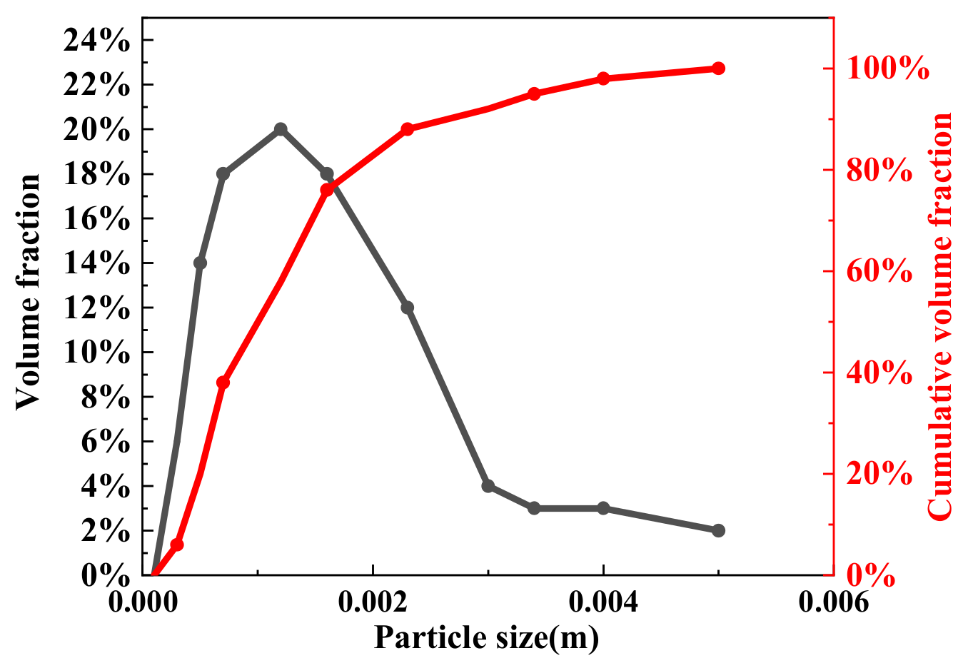
| Diameter of mineral powder | 7.5 × 10⁻⁵~1.5 × 10⁻⁴ m |
| Mineral powder density | 4216.81 kg/m3 |
| Adhesive diameter | 5 × 10⁻³~1 × 10⁻² m |
| Drag model | Wen-Yu |
| Non-dimensional exponent, β | 3 |
| Non-dimensional constant, a | 10−8 |
| Turbulence model | Large eddy simulation (LES) turbulence |
| Maximum momentum of particle collision | 40% |
| Time step | 0.001 s |
| Total time | 2500 s |
| A Reduction Temperature /K | B Reduction Gas Type | C Reduction Pressure/MPa | D Gas Linear Velocity/m/s |
|---|---|---|---|
| A1 A2 A3 | B1 B2 B3 | C1 C2 C3 | D1 D2 D3 |
| 923 1023 1123 | H2 CO Mixture | 0.1 0.2 0.4 | 0.4 0.6 0.8 |
| No. | Reduction Temperature/K | Type of Reducing Gas | Reducing Pressure/MPa | Linear Velocity/m/s | Metallization Rate /% | Simulated Metallization Rate/% |
|---|---|---|---|---|---|---|
| 1 | 1123 | H2 | 0.1 | 0.6 | 76.45 | 86.45 |
| 2 | 1023 | CO | 0.1 | 0.6 | 60.46 | 68.46 |
| 3 | 1023 | H2 + CO | 0.1 | 0.6 | 63.15 | 70.15 |
| 4 | 923 | H2 + CO | 0.2 | 0.6 | 80.04 | 99.13 |
| 5 | 923 | H2 + CO | 0.4 | 0.6 | 81.65 | 99.81 |
| 6 | 1023 | H2 + CO | 0.1 | 0.4 | 51.88 | 58.88 |
| 7 | 1023 | H2 + CO | 0.1 | 0.8 | 60.19 | 69.19 |
| 8 | 1023 | H2 | 0.2 | 0.4 | 56.87 | 62.87 |
| No. | Reduction Temperature/K | Type of Reducing Gas | Reducing Pressure/MPa | Linear Velocity/m/s | Simulation Equilibration Time/s |
|---|---|---|---|---|---|
| 1 | 923 | H2 | 0.2 | 0.6 | 1215 |
| 2 | 1023 | H2 | 0.2 | 0.6 | 990 |
| 3 | 1123 | H2 | 0.2 | 0.6 | 1240 |
| 4 | 923 | H2 | 0.1 | 0.6 | 1255 |
| 5 | 1023 | H2 | 0.1 | 0.6 | 1105 |
| 6 | 1123 | H2 | 0.1 | 0.6 | 1305 |
| No. | Reduction Temperature/K | Type of Reducing Gas | Reducing Pressure/MPa | Linear Velocity/m/s | Simulation Equilibration Time/s |
|---|---|---|---|---|---|
| 7 | 1023 | H2 | 0.1 | 0.6 | 1375 |
| 8 | 1023 | CO | 0.1 | 0.6 | 1675 |
| 9 | 1023 | H2 + CO | 0.1 | 0.6 | 1580 |
| 10 | 1023 | H2 | 0.2 | 0.6 | 1050 |
| 11 | 1023 | CO | 0.2 | 0.6 | 1305 |
| 12 | 1023 | H2 + CO | 0.2 | 0.6 | 1155 |
| No. | Reduction Temperature/K | Type of Reducing Gas | Reducing Pressure/MPa | Linear Velocity/m/s | Simulation Equilibration Time/s |
|---|---|---|---|---|---|
| 13 | 1023 | H2 + CO | 0.1 | 0.6 | 1625 |
| 14 | 1023 | H2 + CO | 0.2 | 0.6 | 1115 |
| 15 | 1023 | H2 + CO | 0.4 | 0.6 | 1050 |
| 16 | 923 | H2 + CO | 0.1 | 0.6 | 1605 |
| 17 | 923 | H2 + CO | 0.2 | 0.6 | 1105 |
| 18 | 923 | H2 + CO | 0.4 | 0.6 | 1055 |
| No. | Reduction Temperature/K | Type of Reducing Gas | Reducing Pressure/MPa | Linear Velocity/m/s | Simulation Equilibration Time/s |
|---|---|---|---|---|---|
| 19 | 1023 | H2 + CO | 0.1 | 0.4 | ---- |
| 20 | 1023 | H2 + CO | 0.1 | 0.6 | 1580 |
| 21 | 1023 | H2 + CO | 0.1 | 0.8 | 1875 |
| 22 | 1023 | H2 | 0.2 | 0.4 | ---- |
| 23 | 1023 | H2 | 0.2 | 0.6 | 1055 |
| 24 | 1023 | H2 | 0.2 | 0.8 | 1400 |
Publisher’s Note: MDPI stays neutral with regard to jurisdictional claims in published maps and institutional affiliations. |
© 2022 by the authors. Licensee MDPI, Basel, Switzerland. This article is an open access article distributed under the terms and conditions of the Creative Commons Attribution (CC BY) license (https://creativecommons.org/licenses/by/4.0/).
Share and Cite
Wan, Z.-w.; Huang, J.-y.; Zhu, G.-m.; Xu, Q.-y. Numerical Simulation of the Operating Conditions for the Reduction of Iron Ore Powder in a Fluidized Bed Based on the CPFD Method. Processes 2022, 10, 1870. https://doi.org/10.3390/pr10091870
Wan Z-w, Huang J-y, Zhu G-m, Xu Q-y. Numerical Simulation of the Operating Conditions for the Reduction of Iron Ore Powder in a Fluidized Bed Based on the CPFD Method. Processes. 2022; 10(9):1870. https://doi.org/10.3390/pr10091870
Chicago/Turabian StyleWan, Zi-wei, Jin-yu Huang, Guo-min Zhu, and Qi-yan Xu. 2022. "Numerical Simulation of the Operating Conditions for the Reduction of Iron Ore Powder in a Fluidized Bed Based on the CPFD Method" Processes 10, no. 9: 1870. https://doi.org/10.3390/pr10091870