An Efficient Ant Colony Algorithm Based on Rank 2 Matrix Approximation Method for Aircraft Arrival/Departure Scheduling Problem

Abstract

The Aircraft Arrival/Departure Problem (AADSP) is the core problem in current runway system, even has become the bottleneck to prevent the improvement of the airport efficiency. This paper studies the single runway AADSP. A Mixed Integer Programming (MIP) model is constructed and an algorithm named Ant Colony based on Rank 2 Matrix Approximation (RMA-AC) method is proposed. Numerical results validate that the new algorithm, as well as the new model, exhibits better performance than CPLEX and the traditional two-phase algorithm. The runway efficiency enhanced by RMA-AC, within 20 s computation, is about 2–5% even for the 800 aircraft sequences. It is a promising method to improve the efficiency of the future aircraft scheduling system.

1. Introduction

With the rapid improvement of social economy and people’s living standards, the air traffic flow has continued to grow in recent years (Boeing [1], Federal Aviation Administration [2]). Although the outbreak of COVID-19 has temporarily limited aviation demand, authoritative forecasts indicate that sharp increase of air traffic will appear after the epidemic (Gudmundsson [3]). How to improve the capacity of the air transportation system will continue to be a significant but challenging problem for governments, airlines and passengers.

Many researches and investigations have pointed out that insufficient throughput of runway is the bottleneck of the air transport system (Bennell et al. [4]). However, the construction of new runways is expensive. For example, the construction of the third runway in Wuhan Tianhe International Airport cost 3.08 billion yuan (Wuhan Network Information Office [5]). Therefore, many experts and scholars attempt to make the most use of the existed runway, that is, to sequence the aircraft on the runway to improve the efficiency of runway utilization. It is known as the Aircraft Arrival/Departure Scheduling Problem (AADSP), or Aircraft Scheduling Problem (ASP) for simple (Beasley et al. [6], Balakrishnan and Chandran [7], Ikli et al. [8]).

ASP aims to take off/land as many aircraft as possible within a given period of time. ASP concerns a given minimum separation time (MST) table.

Table 1. MST (in sec.) between successive aircraft on the same runway for three aircraft types with two status.

			Following
			Arrival			Departure
			A1	A2	A3	D1	D2	D3
Leading		A1	99	133	196	40	40	40
	Arrival	A2	74	107	131	35	35	35
		A3	74	80	98	30	30	30
		D1	50	53	65	60	90	120
	Departure	D2	50	53	65	60	60	90
		D3	50	53	65	60	60	60

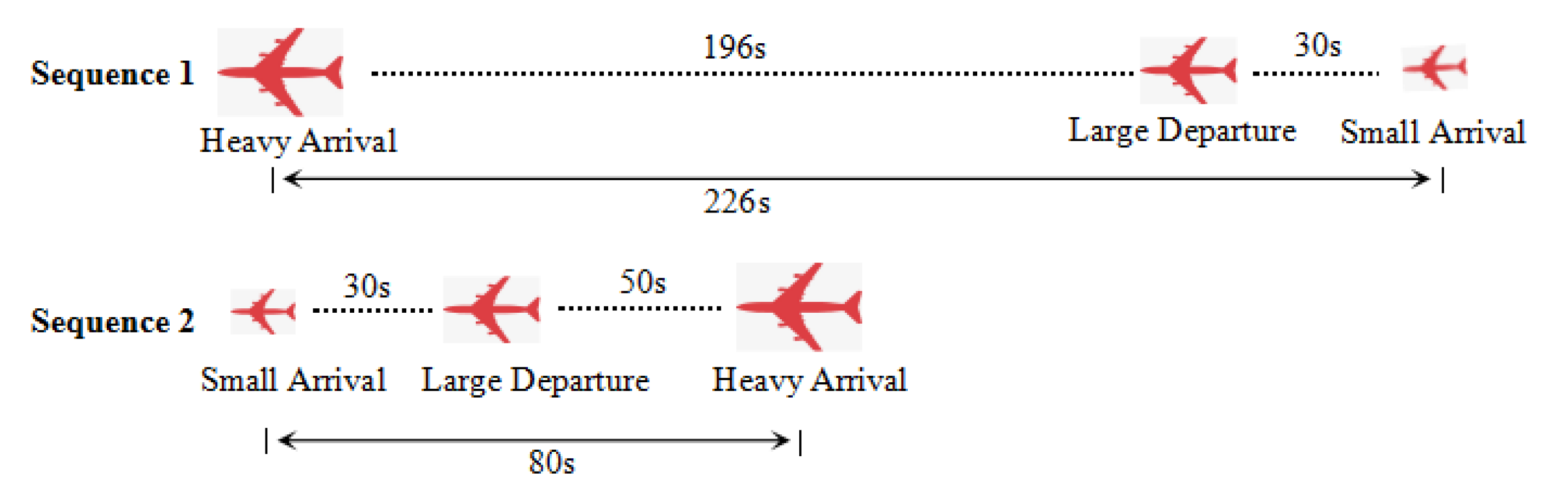
Note: A1-heavy arrival, A2-large arrival, A3-small arrival, D1-heavy departure, D2-large departure, D3-small departure.

illustrates the MST between the successive aircraft concerning three typical aircraft types with arrival or departure status, that is, small arrival, large arrival, heavy arrival, small departure, large departure and heavy departure. The MST table is asymmetrical. If a small arrival aircraft lands after a heavy arrival, the required separation between them is 196s; however, when a heavy arrival aircraft lands after a small arrival, the separation is only 60 s. So a proper scheduling strategy may greatly shorten the makespan. Figure 1 presents two scheduling strategies for the same three aircraft. The strategy of sequences 2 saves more than 65% of time than that of sequence 1.

The asymmetry nature leads ASP to be NP-hard with high computational complexity. There are at most $A_n^n=[n(n-1)(n-2)···1]$ possible sequencing strategies with n aircraft (Beasley et al. [6], Balakrishnan and Chandran [7]). The Branch and Bound (B&B), Ant Colony (AC) and Matrix Approximation (MA) algorithms are the most used solution methods.

Branch and Bound (B&B): Brinton [9] has introduced the first B&B approach for ASP in 1992, which is a foundation tool of the Center TRACON Automation System (CTAS) developed by NASA. Then Beasley et al. [6] proposes an widely cited Mixed Integer Programming (MIP) approach for ASP, and designs the corresponding B&B algorithm. Some additional constraints are added to reduce the zero-one space of the mixed integer formulation. Bennell et al. [4] present an extensive literature overview on B&B. Prakash et al. [10] proposes the B&B algorithm for single runway AADSP, where the data-splitting method is used to reduce the search space. It splits the original sequence into all possible pairs of sub-sequences, and then independently solves each sub-sequence, while ensuring global optimality. Then Prakash et al. [11] extend this method to the multi-runway case. The winter AADSP is studied by Pohl et al. [12]. The B&B algorithm is designed and three pruning tree rules, concerning time windows, separation identical aircraft and dominant snow removal patterns, are used.

Ant colony (AC): Ant colony is firstly adopted by Randall [13] for ASP in 2002. The objective function is to minimize the total penalty costs. Then Zhan et al. [14] combines the AC system with Receding Horizon Control (RHC) for real-time scheduling. By comparing with Hu and Chen [15], it validates that the AC is better than GA under the RHC strategy. Wu et al. [16] extends this method to the multi-runway case, and designs a two-stage RHC based AC algorithm. In the first stage, AC algorithm optimize the aircraft based on single runway problem; in the second stage, the aircraft are assigned to the multi-runway based on the first stage queue and the actual runway occupation. Bencheikh et al. [17] use a bi-level graph to model the multi-runway ASP and designs an AC algorithm. Ants start from a dummy initial node, select a runway, then insert an aircraft in this runway, based on the aircraft priority and the ant colony memory. Numerical results show that their AC finds optimal solution for 80% of the test instances. Bencheikh et al. [18] then study the dynamic ASP and propose a new algorithm named memetic which involves the local heuristic algorithm in AC. Ma et al. [19] uses the AC algorithm for the AADSP, a two-phase algorithm is proposed for the air traffic management. In the first phase, the takeoff aircraft are separated from the original sequence, and AC algorithm is used to schedule the landing sequence. In the second phase, the takeoff aircraft are inserted into the scheduled landing sequence while assure the landing first. A parameter M is set to restrict the time of each landing aircraft moving back from the scheduled time, which is not more than M. This method (named TPLP-M) is used as a comparison in the following numerical study.

Matrix Approximation (MA): The MA method is proposed by Ma et al. [20] and Faye [21]. Ma et al. [20] use a rank 2 matrix to approximate the original Minimum Separation Time (MST) matrix. Then the ASP becomes sequence-independent and thus easier to solve. This method sacrifices the solution quality, but accelerates the computational speed. Faye [21] use the rank 2 matrix approximation method to study the multi-runway scheduling problem where the B&B algorithm is involved in the method. Lidier and Stolletz [22] admit the advantages of this method, but points out that this method will produce certain errors when approximating the matrix. Xu [23] studies the mechanism of errors generating, and use the AC algorithm to repair the accuracy loss. The methods have two steps: first, the aircraft MST matrix is approximated by rank 2 matrix, which similar as Ma et al. [20] and Faye [21]; second, AC algorithm is used to supplement the loss in the matrix approximating process. The numerical study validates that this new algorithm is better than the algorithm in Ma et al. [20] when minimize the makespan.

Other methods: Some other methods for runway and aircraft scheduling see in Anagnostakis and Clarke [24], Liu et al. [25], Atkins and Brinton [26], Bohme [27], Lee [28], Willemain et al. [29], Pinedo et al. [30], Khassiba et al. [31], Huo et al. [32], Yu et al. [33], Ghosh et al. [34]. And some hybrid algorithms are in Eslami et al. [35], Khajehzadeh et al. [36], Khajehzadeh et al. [37].

In this paper, we go on investigating the MA method, and combine it with the AC algorithm to solve AADSP. AC is chosen here because each ant in AC directly returns a sequencing strategy which is a possible choice to increase the precision of the MA method. We firstly generate a rank 2 matrix (denoted by MST${}^{\prime }$) to approximate the actual minimum separation time (MST), where the optimal solution concerning MST${}^{\prime }$ is easy to find when the aircraft time window constraint is ignored and the triangle inequality assumption is not violated. Then we use AC to optimize the AADSP while considering the differences between MST and MST${}^{\prime }$ and the additional constraints. The numerical study validates that this new method has better performance than CPLEX and the two-stage algorithm in Ma et al. [19]. It is a promising method to improve the efficiency of the aircraft scheduling system.

In the remainder of this paper, we use RMA-AC to denote “the AC algorithm based on RMA method” for abbreviation.

This paper is organized as follows. The AADSP is defined in Section 2. In Section 3, the MST constraint is analyzed, and the RMA method is proposed. In Section 4, RMA-AC algorithm is originally designed to solve AADSP. The numerical study is conducted in Section 5, while some conclusions are summarized in Section 6.

2. Problem Definition

2.1. Basic Concepts

(1) First Come First Served (FCFS)

The FCFS strategy is widely used in the airport scheduling system. In the landing case, FCFS is implemented according to the estimated landing time of each aircraft. The estimated landing time is achieved by the aircrafts’ planned arrival route, cruise speed, and the standard procedure descent profile. In the take-off case, the captain proposes to the ATC the time when the aircraft can leave the gate and drive to the runway, so as to determine the take-off FCFS sequence. The advantage of FCFS owes to its simplified operation process to the controller and fairness to each aircraft, while the disadvantage owes to the low runway utilization.

(2) Time Windows Constraint

The time window constraint restricts that the aircraft must take-off/land within its earliest and latest possible take-off/landing time, otherwise insecurity may happen. We use $E_i$ and $L_i$ to indicate the earliest and latest possible takeoff/landing time of the aircraft i, then the actual takeoff/landing time should be restricted within the range of $[E_i,L_i]$. $E_i$ is determined by the factors including the aircraft speed, runway availability, weather factors, scheduling strategy, and so on; while $L_i$ is determined by the factors including aircraft speed, runway availability, limited aircraft fuel, maximum allowable delay time, scheduling strategy, and so on.

(3) Minimum Separation Time (MST)

The aircraft in the air generates wake vortex. If two aircraft get too close, the generated wake will cause dangerous rolling moment to the following aircraft. So the minimum separation must kept between them. The MST is determined by the aircraft weight, type, speed, navigation facilities, and other factors. The aircraft weight is the most important factor relating to the aircraft wake vortex. Generally speaking, heavy aircraft generates stronger wake, and can also bear stronger wake disturbance; while small aircraft are just the opposite. Therefore, the case of a small aircraft following a heavy aircraft (compared with a heavy aircraft following a small) requires greater separation (see in Table 1, and see also in Hancerliogullari et al. [38]).

It is worthy to note that, in AADSP, the triangle inequality for aircraft minimum separation may not satisfy, that is, $d_{ij}<d_{is}+d_{sj},i,j,s\in \Lambda$, where $\Lambda$ is the aircraft sequence set, and $d_{ij}$ is the MST of aircraft i followed by aircraft j. For example, when there are three aircraft for scheduling, which are 1 arrival heavy, 2 small departure, 3 small arrival, then $d_{13}=196>d_{12}+d_{23}=75+60$.

2.2. Problem Description

Suppose there are n aircraft, and they are labeled according to their order in the FCFS sequence. $\Lambda =\{1,2,···,n\}$ denotes the aircraft set. $\pi$ is the final scheduled sequence which indicates the order of all the aircraft. ${\pi }_i$ is the ith aircraft in sequence $\pi$, and its value indicates the order of aircraft ${\pi }_i$ in the original FCFS sequence. For example, ${\pi }_5=6$ means that the fifth aircraft in the scheduled sequence $\pi$ is the sixth aircraft in the FCFS sequence. $d_{{\pi }_i{\pi }_{i+1}}$ denotes the MST between two successive aircraft (${\pi }_i$ and ${\pi }_{i+1}$) in sequence $\pi$. $E_{{\pi }_i}$ and $L_{{\pi }_i}$ are the earliest and latest take-off/landing time of aircraft ${\pi }_i$, respectively. Then the final takeoff/landing time $x_{{\pi }_i}$ for aircraft ${\pi }_i$ can be achieved by

$$x_{{\pi }_i}=\left\{\begin{array}{cc}{E}_{{\pi }_i}\hfill & \mathrm{if}i=1;\hfill \\ \underset{x_{{\pi }_i}\le L_i}{max}\{E_{{\pi }_i},x_{{\pi }_{i-1}}+d_{{\pi }_{i-1}{\pi }_i}\},\hfill & \mathrm{if}i=2;\hfill \\ \underset{x_{{\pi }_i}\le L_i}{max}\{E_{{\pi }_i},x_{{\pi }_{i-1}}+d_{{\pi }_{i-1}{\pi }_i},x_{{\pi }_{i-2}}+d_{{\pi }_{i-2}{\pi }_i}\}\hfill & \mathrm{other}.\hfill \end{array}\right.$$

(1)

The objective function is the makespan (W), which is the takeoff/landing time of the last aircraft in the scheduled sequence $\pi$ (denoted by ${\pi }_{\mathrm{end}}$), that is,

$$\left({\mathrm{MIP}}^1\right)min{W}_{\pi }=x_{{\pi }_{\mathrm{end}}},\forall {\pi }_i\in \Lambda$$

(2)

2.3. Mixed Integer Programming (MIP) Model

Suppose the arrival/departure aircraft set is $\Lambda =\{1,2,···,n\}$. Each aircraft $i\in \Lambda$ has a predefined time window $[E_i,L_i]$. $d_{ij}$ is the MST of aircraft i followed by j, and $x_i$ is the executed take-off/landing time of aircraft i. The MIP model is described in Equations (3)–(8).

The objective function (3) is to minimize the makespan of the final aircraft sequence, which is equivalent to Equation (2). Here, $x_i$ is the takeoff/landing time of aircraft i, and constraint (7) restrict $W\ge x_i$, $i=1,2,···,n$. Thus W is the take-off/landing time of the last aircraft.

Constraint (4) ensures each aircraft i takoff/landing within its time window, which is between the earliest takeoff/landing time $E_i$ and the latest takeoff/landing time $L_i$.

In constraint (5), ${\delta }_{ij}$ is a 0-1 variable. ${\delta }_{ij}=1$ means that aircraft i should takeoff/landing before aircraft j, while ${\delta }_{ij}=0$ means that aircraft i should after j. ${\delta }_{ij}$ and ${\delta }_{ji}$ should not equal to 0 (or 1) at the same time. ${\delta }_{ij}+{\delta }_{ji}=1$ ensures this requirement. U is the domain of all possible $(i,j)$ in ${\delta }_{ij}$, that is $U=\left\{\right(i,j):i,j\in \Lambda ,i\ne j\}$.

Constraint (6) ensures the MST constraint, where $d_{ij}$ is the MST of aircraft j following i. There are two cases

(i) Aircraft i before j (${\delta }_{ji}=0$). Then $x_j\ge x_i+d_{ij}$ ensures the separation $d_{ij}$ between aircraft i and j.

(ii) Aircraft i after j (${\delta }_{ji}=1$). Then $x_j\ge x_i+d_{ij}-M$, which is ineffective when M is large enough.

For the special case of triangle inequality not satisfying, constraint (6) ensures all aircraft in the runway satisfying MST constraint, and thus involves the special case.

Constraint (8) is the definition and restriction of all variables.

$$\left({\mathrm{MIP}}^2\right)minW$$

(3)

$$\mathrm{s}.\mathrm{t}.E_i\le x_i\le L_i;\forall i\in \Lambda$$

(4)

$${\delta }_{ij}+{\delta }_{ji}=1;\forall (i,j)\in U$$

(5)

$$x_j-x_i\ge d_{ij}-{\delta }_{ji}·M;\forall (i,j)\in U$$

(6)

$$W\ge x_i;\forall i\in \Lambda$$

(7)

$$x_i\ge 0,W\ge 0,{\delta }_{ij}=0,1;\forall (i,j)\in U$$

(8)

3. Rank 2 Matrix Approximation (RMA) Method

The RMA method is originally proposed by Ma et al. [20] and Faye [21]. Firstly, it generates a new rank 2 matrix (denoted by MST${}^{\prime }$), and the ASP concerning this new MST${}^{\prime }$ is linearly solvable. Secondly, MST${}^{\prime }$ limitlessly approximates the actual MST until they get close enough. Finally, the solution of ASP concerning the new MST${}^{\prime }$ is exact the (hypo-)optimal solution of that concerning the actual MST, that is, the traditional difficult ASP (concerning MST) is transferred to an easier ASP (concerning MST${}^{\prime }$). Following are the MST${}^{\prime }$ generating process and some useful properties.

3.1. Construction of Rank 2 Matrix Approximation Method

An important factor leading to the high complexity of ASP is the asymmetric nature of the MST matrix. The idea of the RMA method is to approximate the actual MST matrix by a rank 2 matrix, thus the ASP is simplified (Ma et al. [20], Faye [21], Xu [23]).

The MST matrix is used to avoid the wake-vortex effect and ensure the safety of the following aircraft (Xu [23]). As we known, heavy aircraft can generate and bear stronger vortex, while small aircraft just the opposite. 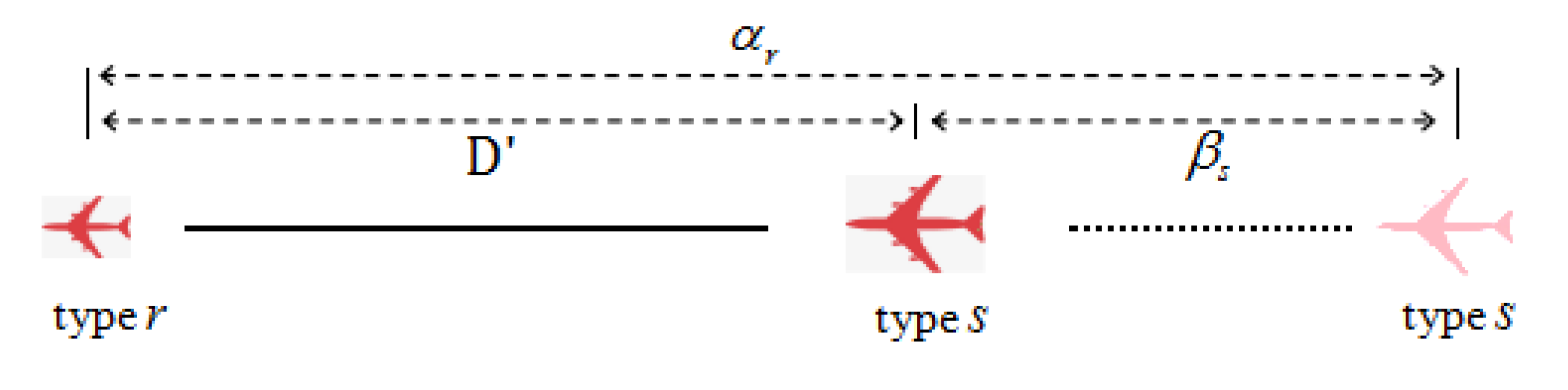Then we can divide the MST matrix into two parts, where ${\alpha }_r$ denotes the ability of the leading aircraft of type r generating vortex and ${\beta }_s$ denotes the ability of the following aircraft of type s bearing vortex. Thus the new MST matrix is achieved by $D_{rs}^{\prime }={\alpha }_r-{\beta }_s$ (see in Figure 2). Here, $D^{\prime }$ is the new rank 2 matrix, which is achieved by $\left({\mathrm{LP}}^3\right)$. $\Theta$ is the aircraft type set, and suppose there are p type of aircraft.

The objective function (9) is to minimize the total differences between the original MST matrix D and the lately generated rank 2 matrix $D^{\prime }$. $\Delta D$ measures the differences between D and $D^{\prime }$ (see in Equation (10)).

Constraint (11) is the lately generated rank 2 matrix $D^{\prime }$, where each element in it can be divided into two parts. The first part (denoted by ${\alpha }_r$) models the ability of the leading aircraft of type r to generate vortex, and the second part (denoted by ${\beta }_s$) models the ability of the following aircraft of type s to bear vortex.

Constraint (12) restricts the main variables ($\Delta D_{rs}$, ${\alpha }_r$ and ${\beta }_s$) non-negative. $\Delta D_{rs}\ge 0$ makes each element in $D^{\prime }$ not bigger than the corresponding element in D, which ensures the following theorem 1 and the condition (3) in theorem 3.

$$\left({\mathrm{LP}}^3\right)min{\mathsf{\Sigma }}_{r=1}^p{\mathsf{\Sigma }}_{s=1}^p\Delta D_{rs}$$

(9)

$$\mathrm{s}.\mathrm{t}.D_{rs}-D_{rs}^{\prime }=\Delta D_{rs};\forall r,s\in \Theta$$

(10)

$${\alpha }_r-{\beta }_s=D_{rs}^{\prime };\forall r,s\in \Theta$$

(11)

$$\Delta D_{rs}\ge 0,{\alpha }_r\ge 0,{\beta }_s\ge 0;\forall r,s\in \Theta$$

(12)

We can also use $\Delta$MST to denote $\Delta D$. Then there comes three main types of ASP, which are ASP-MST, ASP-MST${}^{\prime }$, and ASP-$\Delta$MST. ASP-MST means that in the ASP the separation between the successive aircraft is determined by MST; ASP-MST${}^{\prime }$ means that determined by MST${}^{\prime }$; and ASP-$\Delta$MST means that determined by $\Delta$MST.

Following, $D_{rs}$, $D_{rs}^{\prime }$ and $\Delta D_{rs}$ denotes, respectively, the element in the matrices of MST, MST${}^{\prime }$ and $\Delta$MST when an aircraft of type r is followed by another of type s.

3.2. Important Property of ASP-MST${}^{\prime }$

The rank 2 matrix MST${}^{\prime }$ generated above has two main properties to make optimization easier. Firstly, ASP-MST${}^{\prime }$ is the lower-bound of ASP-MST. Secondly, ASP-MST${}^{\prime }$ is sequence-independent and easier to solve (while ASP-MST is sequence-dependent). When the RAM method optimizes the original ASP-MST, it first finds the lower-bound via ASP-MST${}^{\prime }$, and then generates a solution approximating this lower bound to form a good final solution.

In this subsection, the time window constraint is assumed ignored and the triangle inequality for MST is assumed not violated, for simple. The case of violating the two assumptions is discussed in Section 4 when designing the AC algorithm for real scheduling. Theorems 1 and 2 explain the two properties of ASP-MST${}^{\prime }$ (see their proofs in Ma et al. [20]). Theorem 3 supports the approximating process (see its proof in Xu [23]). Here, $W_{\pi }$, $W_{\pi }^{\prime }$ and $\Delta W_{\pi }$ are the makespan of sequence $\pi$ in ASP-MST, ASP-MST${}^{\prime }$ and ASP-$\Delta$MST, respectively. $\Theta$ is the aircraft type set. When considering Table 1, we have $\Theta =\left\{1\right(A1),2(A2),3(A3),4(D1),5(D2),6(D3\left)\right\}$.

Theorem 1.

The makespan of each sequence π in ASP-MST${}^{\prime }$ is the lower bound of π in ASP-MST, that is, $W_{\pi }^{\prime }\le W_{\pi }$.

Theorem 2.

The optimal solution of minimizing makespan for ASP-$MS{T}^{\prime }$ only depends on the first and the last aircraft in the final sequence, if the time window constraint is assumed ignored, the triangle inequality for MST is assumed not violated, and ${\alpha }_i$ and ${\beta }_i$ are given constant, $\forall i\in \Theta$.

Theorem 2 simplifies ASP-MST${}^{\prime }$ when the time window constraint is ignored and triangle inequality is not violated. Theorem 3 explains the relationship of ASP-MST and ASP-MST${}^{\prime }$, and presents sufficient condition of the optimal solution of ASP-MST.

Theorem 3.

When the time window constraint is ignored and triangle inequality is not violated, the sequence Π is optimal (with minimized makespan) in ASP-MST model if the following three requirements are satisfied.

(1)

Sequence Π is the optimal sequence in ASP-$MS{T}^{\prime }$ model;

(2)

Sequence Π has 0 makespan in ASP-$\Delta MST$ model, i.e., $\Delta W_{\Pi }=0$;

(3)

All elements in ΔMST are nonnegative, i.e., all elements in MST ${}^{\prime }$ are not bigger than the corresponding elements in MST.

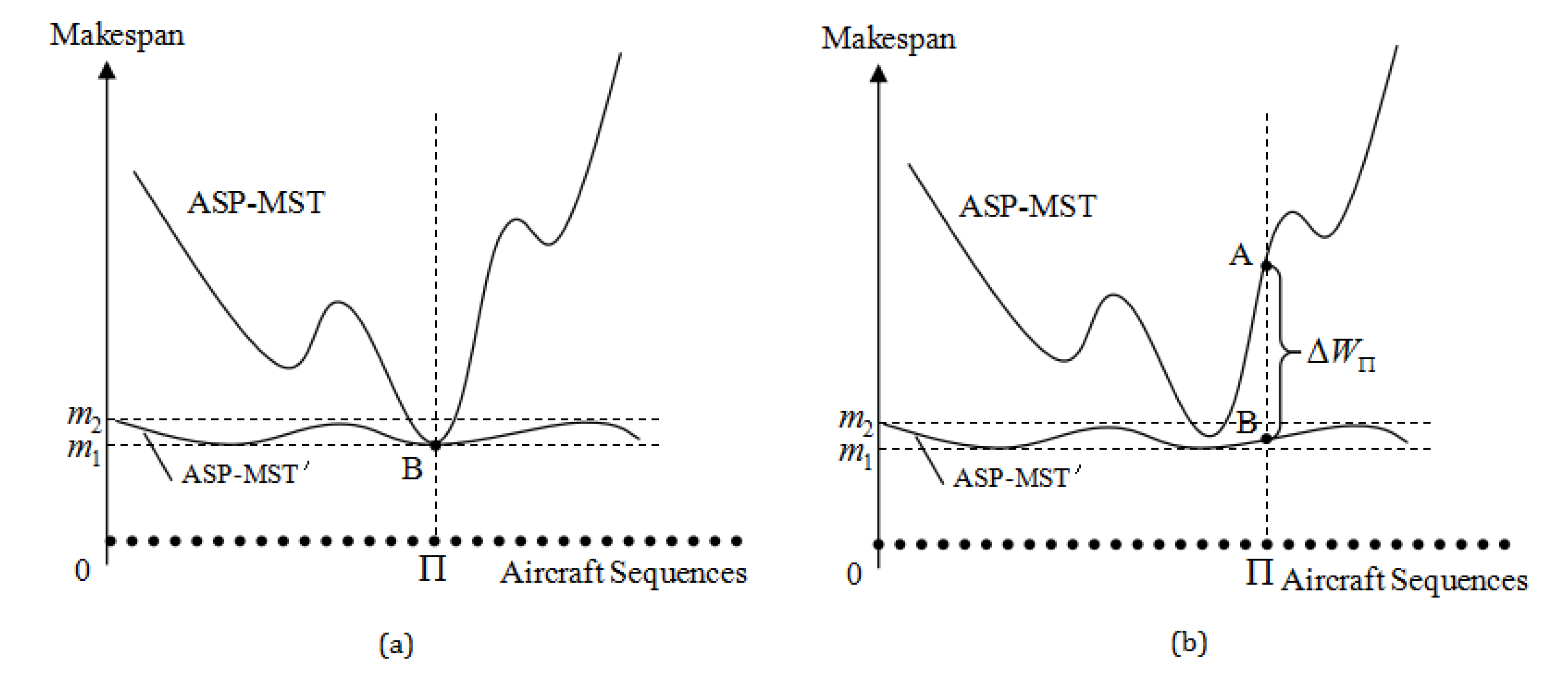
Figure 3a illustrates the relationship between ASP-MST and ASP-MST${}^{\prime }$. Requirement (3) shows the ASP-MST${}^{\prime }$ curve always below ASP-MST curve. Requirements (2) means that ASP-MST curve is tangent to ASP-MST${}^{\prime }$ curve at the point representing sequence $\Pi$. Requirement (1) shows that the ASP-MST${}^{\prime }$ curve reaches the bottom at the point representing sequence $\Pi$. Thus ASP-MST is minimized at the point of $\Pi$.

If requirement (1) is not satisfied, but requirements (2) and (3) are satisfied, by a sequence $\Pi$, then $\Pi$ is strongly hypo-optimal. Here, “strongly hypo-optimal” means that the sequence’s optimality is only determined by its first and last aircraft. A sequence in ASP-MST${}^{\prime }$ is at least strongly hypo-optimal when the time window constraint is ignored and triangle inequality is not violated (Theorem 1).

Based on the above theorems, the optimization of ASP based on the RMA method contains three steps. First, for a given aircraft sequence, we use ${\mathrm{LP}}^3$ to construct a rank 2 matrix $D^{\prime }$ satisfying the requirement (3) of theorem 3. Second, optimize $\mathrm{ASP}\text{-}\Delta \mathrm{MST}$ according to the requirement (2) in theorem 3 to minimize the makespan of $\mathrm{ASP}\text{-}\Delta \mathrm{MST}$. Finally, the optimal or nearly optimal solution is obtained (that is, find the aircraft sequence $\Pi$ so that $\Delta W_{\Pi }$ in Figure 3b is minimized). Following we use AC algorithm to optimize $\mathrm{ASP}\text{-}\Delta \mathrm{MST}$ and consider the case with time window constraint and triangle inequality violation.

4. Ant Colony Algorithm Based on RMA Method

As shown above, RMA method generates rank 2 matrices of MST${}^{\prime }$. Then we can optimize ASP-MST${}^{\prime }$ which is sequence-independent and easier to solve, but a significant loss of precision may happen between MST and MST${}^{\prime }$. To overcome it, the AC algorithm is used to supplement the precision via considering $\Delta \mathrm{MST}(=\mathrm{MST}-{\mathrm{MST}}^{\prime })$. The time window constraint and triangle inequality violation are also considered. Numerical results in Section 4 validate the efficiency of this new algorithm, named RMA-AC.

4.1. RMA-AC Algorithm Construction

Following introduces the RMA-AC algorithm for AADSP. AC is a famous meta-heuristic algorithm via modeling the ants behavior searching for food. It is originally developed for the Traveling Salesman Problem (TSP), which aims to find the shortest route for a traveler visiting each node once and only once in a graph, starting and finishing at the same node (Dorigo [39]).

The AADSP is similar as an open TSP (the tour does not return to the origin), where the runway is regarded as a traveler and aircraft as nodes (Randall [13], Bennell et al. [4]). The time window constraint and triangle inequality violation are considered. The objective is to minimize makespan in Equation (2). The ants are expected to visit out all nodes as soon as possible, which is equivalent to the runway landing as many aircraft as possible. Following is the techniques setting for RMA-AC.

(1) Aircraft Sequences Classification

The aircraft with the same type are not expected to overtake each other, so they are put together to construct subsequences (${ϝ}^r$) according to their orders in the FCFS sequence ($ϝ$). Each time only the first ant-unvisited aircraft in ${ϝ}^r$ is chosen to take-off/land so that the overtaking of aircraft with the same type is avoided. Since there are p aircraft types, we get p subsequences, which are ${ϝ}^1$, ${ϝ}^2$, $···$, ${ϝ}^p$. All aircraft in ${ϝ}^r$ have the same aircraft type of r, $r\in \Theta$. ${ϝ}_i^r$ denotes the ith aircraft in ${ϝ}^r$.

For example, a FCFS sequence is of types $1,5,2,1,2,2,1,5$, $\Theta =\{1,2,3,4,5,6\}$. Then there are 6 subsequences. ${ϝ}^1$ is constructed by the 1st, 4th and 7th aircraft in FCFS according to their order; ${ϝ}^2$ is by the 3rd, 5th and 6th aircraft; ${ϝ}^3$ and ${ϝ}^4$ are empty sets, ${ϝ}^5$ is constructed by the 2nd and 8th aircraft, and ${ϝ}^6$ is also an empty set.

(2) Ants Initialization. The initial pheromone in each arc is set as ${\tau }_0(i,j)=1$, $\forall i\ne j$. Here i and j are the nodes (aircraft), and arcs are imagined between nodes. $L^s=\{L_1^s,L_2^s,···,L_p^s\}$ is an aircraft set for the ant s’s next possible visiting. At the starting, $L_r^s={ϝ}_1^r,\forall r\in \Theta$, and each ant s randomly visits an aircraft in $\{{ϝ}_1^1$, ${ϝ}_1^2$, $···$, ${ϝ}_1^p\}$. After ant s visiting ${ϝ}_1^r$, we set $L_r^s:={ϝ}_2^r$; after visiting ${ϝ}_2^r$, we then set $L_r^s:={ϝ}_3^r$; and so on until all aircraft in ${ϝ}^r$ are visited.

(3) State Transition Rule. After ant s visiting aircraft i, it randomly selects the next allowable aircraft j to visit according to $\mathrm{Pb}(i,j)$.

$$\begin{array}{c}\hfill \begin{array}{c}\hfill \mathrm{Pb}(i,j)=\left\{\begin{array}{cc}\frac{{\left[\tau (i,j)\right]}^{\alpha }{\left[\eta (i,j)\right]}^{\beta }}{{\sum }_{u\in L^s}{\left[\tau (i,u)\right]}^{\alpha }{\left[\eta (i,u)\right]}^{\beta }},\hfill & \mathrm{if}j\in L^s\hfill \\ 0,\hfill & \mathrm{otherwise}\hfill \end{array}\right.\end{array}\end{array}$$

(13)

where $L^s$ is the allowable aircraft which follows aircraft i. $\tau (i,j)$ is the existed pheromone in arc $(i,j)$, and $\eta (i,j)$ is the heuristic information factor. The parameters $\alpha$ and $\beta$ determine the relative importance of $\tau$ versus $\eta$. The heuristic information $\eta (i,j)$ is set as

$$\eta (i,j)=\left\{\begin{array}{cc}\frac{1}{\Delta d_{ij}+max(0,E_j-x_i)+1},\hfill & i={\pi }_1\hfill \\ \frac{1}{max\{\Delta d_{ij},\Delta d_{i-1,j}-\Delta d_{i-1,i}\}+max(0,E_j-x_i)+1},\hfill & i\ge {\pi }_2\hfill \end{array}\right.,$$

(14)

because there are three main factors affecting the final makespan, which are the nonnegative number in $\Delta$MST (denoted by $\Delta d_{ij}$), the time window constraint (denoted by $max(0,E_j-x_i)$), and the triangle inequality violation (denoted by $max\{\Delta d_{ij},\Delta d_{i-1,j}-\Delta d_{i-1,i}\}$). The denominator is set as $+1$ to avoid the infeasible case of 0 denominator. In the actual computing, a simple setting may be more effective, which is

$$\mathrm{OR}\eta (i,j)=\frac{1}{\Delta d_{ij}+max(0,E_j-x_i)+1}.$$

(15)

It weakens the effect of triangle inequality violation in the state transition process. The final makespan computing should be added when ants complete their tours.

(4) Pheromone Updating Rules. The pheromone updating is carried out on each arc $(i,j)$ as Equation (16) after all ants completing their tours.

$${\tau }_{ij}^{t+1}=(1-\gamma ){\tau }_{ij}^t+\Delta {\tau }_{ij}$$

(16)

where ${\tau }_{ij}^t$ is the original pheromone in arc $(i,j)$, and ${\tau }_{ij}^{t+1}$ is the updated pheromone. $(1-\gamma ){\tau }_{ij}^t$ models the pheromone evaporation, where the evaporation ratio is $(1-\gamma )$. $\Delta {\tau }_{ij}$ denotes the lately released pheromone. $\Delta {\tau }_{ij}={\sum }_s\Delta {\tau }_{ij}^s$, and $\Delta {\tau }_{ij}^s$ is defined, for an ant s, as

$$\begin{array}{c}\hfill \begin{array}{c}\hfill \Delta {\tau }_{ij}^s=\left\{\begin{array}{cc}\frac{Q}{x_{{\pi }_{\mathrm{end}}}^s},\hfill & \mathrm{if}\mathrm{arc}(i,j)\mathrm{is}\mathrm{visited}\mathrm{by}\mathrm{ant}s\hfill \\ 0,\hfill & \mathrm{otherwise}\hfill \end{array}\right.\end{array}\end{array}$$

(17)

where $x_{{\pi }_{\mathrm{end}}}^s$ is the tour makespan achieved by Equation (1) for ant s, and Q is a given constant.

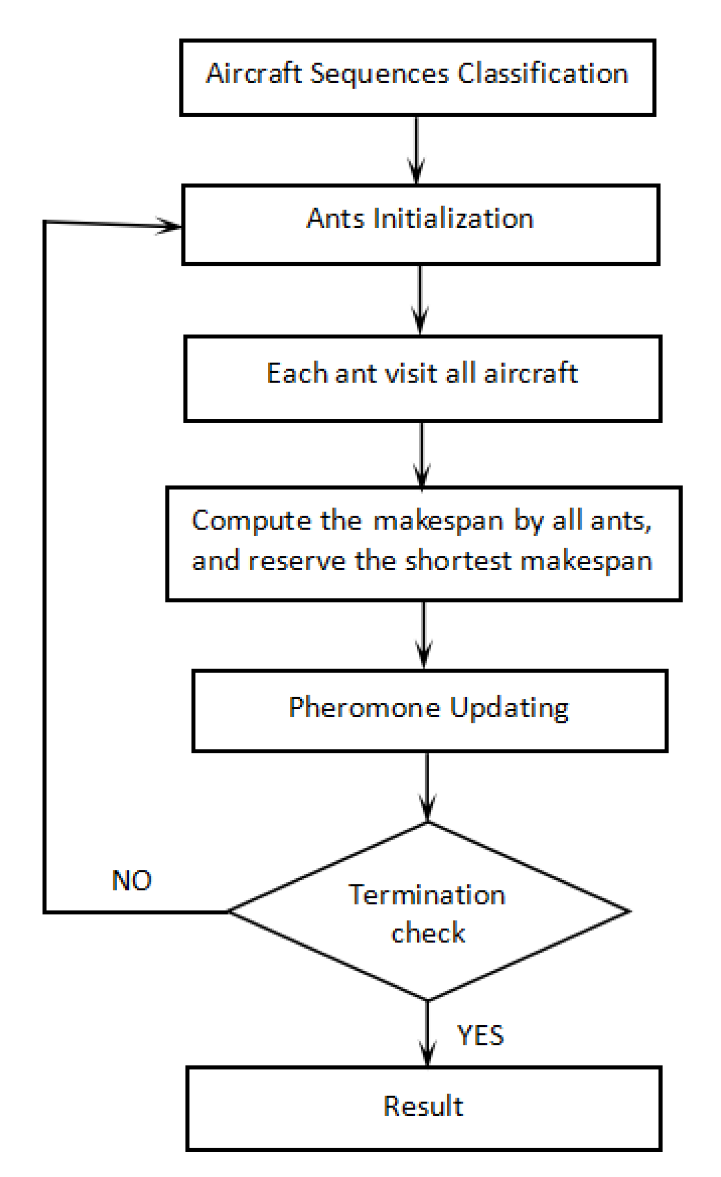
4.2. Complete AC Algorithm

The complete RMA-AC algorithm is explained as follows, see also in Figure 4.

Step 1. Initialization. There are m ants traveling between aircraft. The aircraft sequence is divided into p subsequences according to Section 4.1(1). $L^s=\{L_1^s,L_2^s,···,L_p^s\}$ is the possible aircraft set for ant s’s next visiting. At the starting, each ant s randomly selects an aircraft in $L^s$ to visit. If $L_i^s={ϝ}_1^i$ is chosen, we set $L_i^s={ϝ}_2^i$.

Step 2. Each ant s randomly visits the next aircraft in $L^s$ by Equations (13) and (15). After s visiting $L_i^s={ϝ}_j^i$, set $L_i^s:={ϝ}_{j+1}^i$. If all aircraft in ${ϝ}^i$ have been visited ($j+1>|{ϝ}^i|$), delete $L_i^s$ from $L^s$.

Step 3. If all aircraft in $L^s$ have been visited by ant s ($L^s=\varnothing$), go to Step 4; otherwise ($L^s\ne \varnothing$), go to Step 2.

Step 4. Calculate out ant s’s tour makespan $x_{{\pi }_{\mathrm{end}}}^s$ by Equation (1), then find the shortest tour ${min}_s{x}_{{\pi }_{\mathrm{end}}}^s$. Compare it with the historical shortest tour, and reserve the shorter one.

Step 5. Update the pheromone ${\tau }_{ij}$ by Equations (16) and (17).

Step 6. Termination check. If the termination criteria of the limit time is met, then break the loop and return the final result. Otherwise, go to Step 1.

5. Numerical Study

In this section, two types of data are used to evaluate the algorithm. One is the fixed date given by the literature [19], and the other is the random data generated according to literature [38]. Here, 1, 2 and 3 represent $heavy$, $large$ and $small$ type of landing aircraft, respectively; 4, 5 and 6 represent $heavy$, $large$ and $small$ type of takeoff aircraft, respectively. The parameters of RMA-AC algorithm, as well as TPLP-M algorithm in [19], are set as $m=150$, $\alpha =1$, $\beta =4$, $\gamma =0.1$, $Q=100$. The completion time of FCFS is calculated out by Equation (1), where $\pi$ is replaced by FCFS. Matlab 7.11.0 and CPLEX Optimization Studio 12.5 are used for programming. The computation is carried out in the personal computer with Intel(R) Core(TM) i3-2310M CPU @ 2.10 GHz 2.10 GHz, RAM 4.00GB and Windows 7 OS.

5.1. Test of Fixed Aircraft Sequence

The data in the literature [19] is used for computation, which contains 40 aircraft in total for take-off and landing.

Table 2. RMA-AC, TPLP-M and CPLEX to minimize makespan for the given data within 20 s.

Data			FCFS	CPLEX		TPLP-M		RMA-AC
No.	Aircraft	Earliest	Executed	No.	Executed	No.	Executed	No.	Executed
	Type	Time (s)	Time (s)		Time (s)		Time (s)		Time (s)
1	2	71	71	1	71	2	128	3	154
2	2	128	178	2	178	3	202	1	287
3	1	154	252	3	252	1	335	6	361
4	5	348	348	4	348	4	370	4	401
5	4	353	408	5	408	6	420	2	494
6	1	355	458	6	458	5	460	5	529
7	1	474	557	7	557	7	519	7	579
8	1	622	656	8	656	8	633	9	628
9	4	628	696	10	696	9	673	8	678
10	6	640	816	9	756	11	829	10	748
11	3	651	881	11	821	10	859	11	874
12	4	734	911	12	851	12	919	12	904
13	4	807	971	13	911	15	1024	13	964
14	4	1011	1031	14	1011	13	1059	15	1017
15	2	1013	1084	15	1064	16	1131	14	1052
16	2	1113	1191	16	1171	14	1166	16	1124
17	5	1160	1226	17	1206	20	1262	18	1161
18	4	1161	1286	20	1302	17	1292	21	1224
19	4	1175	1346	18	1332	21	1342	19	1264
20	3	1221	1411	19	1392	18	1382	20	1420
21	1	1224	1485	22	1445	23	1447	17	1450
22	2	1404	1618	21	1519	19	1487	22	1503
23	1	1430	1692	23	1618	22	1580	23	1577
24	4	1520	1732	24	1658	24	1615	24	1617
25	5	1526	1822	27	1717	26	1665	26	1676
26	1	1599	1872	25	1757	25	1705	25	1716
27	1	1699	1971	28	1816	27	1764	27	1775
28	1	1744	2070	30	1856	30	1814	30	1815
29	2	1807	2203	26	1915	28	1864	29	1908
30	6	1814	2238	31	1955	31	1904	31	1943
31	6	1874	2298	29	2048	29	1997	28	1993
32	5	1959	2358	32	2083	32	2032	32	2033
33	4	2082	2418	33	2143	33	2092	33	2093
34	3	2195	2483	34	2208	34	2224	34	2195
35	6	2241	2538	35	2263	35	2254	35	2241
36	1	2250	2588	37	2328	37	2322	37	2306
37	3	2283	2784	38	2360	38	2360	38	2360
38	5	2360	2814	36	2410	36	2410	36	2410
39	5	2379	2874	39	2450	39	2450	39	2450
40	4	2392	2934	40	2510	40	2510	40	2510
makespan(s)			2934		2510 *		2510 *		2510 *
CPU Time(s)					1.8		20		20

Note: 1-Heavy Arrival, 2-Large Arrival, 3-Small Arrival, 4-Heavy Departure, 5-Large Departure, 6-Small Departure, * represents the best solution.

illustrates the final results by CPLEX, TPLP-M and RMA-AC algorithms. It is clear that all of the three algorithms find the optimal solution within 20 s. The reason of setting 20 s is because the air-traffic controller should make quick decision when scheduling the aircraft. A decision cost more than 20 s time of computing loses practical value.

In order to prove the effectiveness and stability of TPLP-M and RMA-AC algorithms, the data in Table 2 is tested for 20 times. The average values, worst solution and the best solution are exhibited (see in

Table 3. Solution quality of RMA-AC, TPLP-M and CPLEX with the time limit of 20 s.

Algorithm	Worst	Best	Average	Average	Runway
	Solution	Solution	Value	CPU Time	Enhance
CPLEX	2510	2510	2510	2	14.5%
TPLP-M	2618	2510	2559	10	12.8%
RMA-AC	2533	2510	2525	10	13.9%
TPLP-M	2627	2510	2545	20	13.3%
RMA-AC	2531	2510	2518	20	14.2%
TPLP-M	2611	2510	2568	60	12.5%
RMA-AC	2526	2510	2517	60	14.2%

). When the CPU computing time is 10 s, 20 s and 60 s, all the solutions obtained by RMA-AC algorithm have better performance than TPLP-M algorithm

In order to test the convergence of the RMA-AC algorithm, Figure 5 records the average sequence makespan in each generations. It is clear that the results returned by the RMA-AC gradually converges with the increase of the ants generations.

5.2. Test of Random Aircraft Sequences

The random data is generated according to literature [38]. In the sequence, six types of aircraft are randomly generated, and the arrival and departure aircraft both accounts for 50%. The heavy aircraft accounts for 50%, the large aircraft accounts for 30%, and the small aircraft accounts for 20%. The earliest arrival/departure time $E_i$ follows the discrete uniform distribution, which is a random number in the interval of $[0,65n]$ (n denotes the number of aircraft). The latest arrival/departure time is the earliest arrival/departure time plus 60 min. The CPU computing time is restricted 20 s. The main reason is that the aircraft scheduling decision is a real-time decision-making problem, which need quickly calculated results. Decision with more than 20 s time of computing often loses practical value since the aircraft has changed its position for a long distance.

Table 4. A comparison of the solution by the three methods for the random data.

	FCFS	CPLEX		TPLP-M		RMA-AC
Aircraft	Makespan	Runway	Time	Runway	Time	Runway	Time
Number	(s)	Enhance	(s)	Enhance	(s)	Enhance	(s)
40	3188	10.87% *	2	10.36%	20	10.64%	20
80	5984	5.73% *	7	4.81%	20	5.43%	20
120	8832	4.51% *	10	3.65%	20	4.45%	20
160	11,846	4.87%	20	4.65%	20	5.11%	20
200	14,664	4.48%	20	3.78%	20	4.71%	20
240	17,498	2.61%	20	2.70%	20	3.58%	20
280	20,838	2.64%	20	4.84%	20	5.32%	20
320	23,380	3.16%	20	3.58%	20	4.29%	20
360	26,363	1.88%	20	3.28%	20	3.92%	20
400	29,111	1.44%	20	2.14%	20	3.06%	20
440	31,995	1.52%	20	2.37%	20	3.17%	20
480	34,658	0.81%	20	1.93%	20	2.69%	20
520	37,440	0.49%	20	1.67%	20	2.54%	20
560	40,257	0.48%	20	1.88%	20	2.64%	20
600	43,873	0.32%	20	3.03%	20	3.65%	20
640	46,595	0.19%	20	2.88%	20	3.72%	20
680	49,434	0.25%	20	2.39%	20	3.25%	20
720	52,378	0.26%	20	2.46%	20	3.18%	20
760	54,940	0.50%	20	2.02%	20	2.89%	20
800	58,038	0.39%	20	2.47%	20	3.40%	20

Note: * labels the optimal solution, underline labels the best solution among three methods.

and Figure 6 show the results of 20 groups with the number of aircraft from 40 to 800. The data in each group were tested for 5 times and the average value is illustrated.

By comparing the results of three methods of CPLEX, TPLP-M and RMA-AC, we can see that the three methods are obviously better than the FCFS algorithm which is widely used in the current runway system. When the number of aircraft is less than or equal to 120, CPLEX gives the best results, and the runway efficiency is improved by about 4–11%. When the number of aircraft is greater than 120, RMA-AC gives the best solution, and the runway efficiency is improved by about 2–5%. By comparing the results of TPLP-M and RMA-AC, it is obvious that the latter has better performance than the former one.

6. Conclusions and Future Work

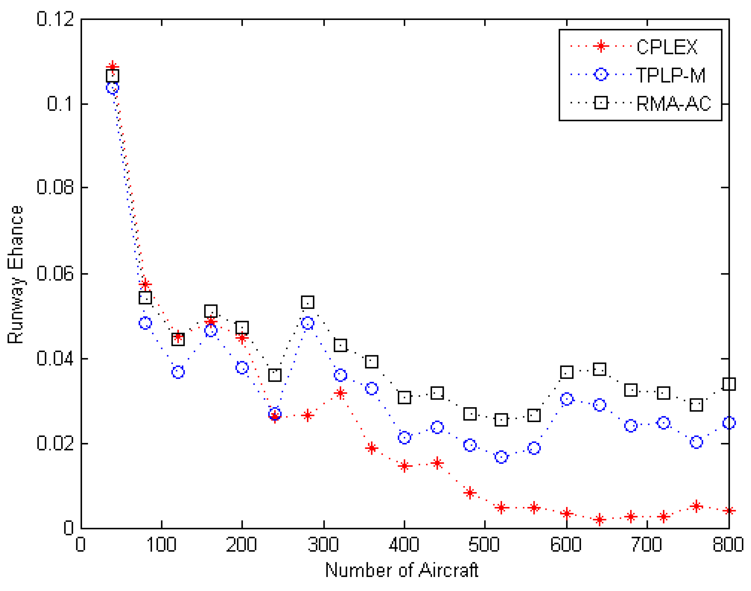
The Aircraft Scheduling Problem (ASP) is the key problem determining airport scheduling efficiency. This paper studies the single runway Aircraft Arrival/Departure Scheduling Problem (AADSP). A Mixed Integer Programming (MIP) model is constructed, and three methods are used, which are the classical Two-Phase with Landing Priority (TPLP-M) algorithm, Ant Colony based on Rank 2 Matrix Approximation (RMA-AC) and the CPLEX optimizer. Numerical experiments show that the three methods can improve the efficiency of runway scheduling. When the number of aircraft is not more than 120, the CPLEX solution is the best; When the number of aircraft is more than 120, the RMA-AC solution is the best. These methods have a positive effect on optimizing the current airport scheduling system, improving the efficiency of runway scheduling and reducing aircraft delay. Numerical result also validates that RMA-AC has better performance than TPLP-M.

There are some research directions for the future study. Firstly, a more efficient algorithm can be designed to improve the efficiency of solution, such as combining the RMA methods with other heuristic algorithm for optimization to get higher efficiency. Secondly, considering the terminal area structure and runway structure, a practical model suitable for a specific airport can be established, such as multi-runway scheduling model. Thirdly, AADSP can be carried out under specific scenarios, such as in busy hours, under emergencies, in the epidemic prevention and control environment. In addition, extending the RMA method to solve other combinatorial optimization problems is also challenging and interesting.