Design and Control Applied to an Extractive Distillation Column with Salt for the Production of Bioethanol

Abstract

Extractive distillation with salts, unlike other dehydration technologies, is better due to the null toxicity that exists in the distillate, since salt cannot be evaporated. With this distillation technology, it is possible to obtain a high concentration of ethanol, however, there are still problems in the control of the distillation columns in the presence of disturbances. The present work deals with the simulation and control of an extractive distillation column using CaCl${}_2$ as a separating agent, for which the Aspen Dynamics^® simulator is used. The measurement and control of the ethanol composition are carried out by means of temperature, in addition, four control structures are evaluated and compared. These structures are L, D, LV, and DV, which are the most common in conventional distillation, and their performance is measured by means of deterministic indicators applying changes (disturbances) of composition and the flow rate in the main feed of the column. The most relevant results of this work lead to the fact that by applying a controller, it is possible to maintain the desired purity above the international purity standards (99% ethanol) that govern biofuels.

1. Introduction

In recent years, research has focused on the search for alternative sources of renewable energy. This is to reduce the dependence on fossil fuels and the greenhouse gas emissions derived from them. To reduce this dependence on fossil fuels, bioethanol has been introduced, produced through fermentation technologies from sugars and starches from raw materials, such as cane, corn, wheat, beet, barley, and sorghum, among others. This type of bioethanol production from these raw materials is known as first-generation biofuel, there are also second- and third-generation biofuels, which use materials, such as plants, trees, animal waste, algae, marine plants, or any other type of vegetable or animal waste. In addition, another type of raw material that is being used recently is the food waste that we generate throughout the food supply chain, from production to human consumption. This type of raw material is known as biomass and is divided into vegetable and lignocellulosic [1,2,3,4,5,6,7].

To produce this type of bioethanol, it is necessary to remove excess water from the ethanol-water mixture produced by fermentation. Depending on the technique used to ferment, the raw material, the bacteria used, and the environmental conditions, it can produce between 3% and 15% molar fraction [8,9]. This concentration is too low to be used as a fuel or additive, because when burned it will not have the same efficiency; that is, it will contain most of the water vapor and this will prevent the ignition and burning of the fuel, not to mention the damage that it can cause inside the engine due to the condensation of the water vapor. Therefore, to be used as a fuel or additive, bioethanol must have a purity equal to or greater than 99.5 wt%, in accordance with international standards (EN 15376; ASTMD 5798-11) [10,11].

To achieve the concentration required by the aforementioned standards, it is necessary to dehydrate the ethanol using non-ideal mixture separation technologies that allow changing or correcting the non-ideal VLE (vapor-liquid equilibrium) of the ethanol-water system to an ideal VLE. As has been mentioned and described in different articles, the ethanol-water mixture is a non-ideal mixture that at a composition of 89% molar fraction of ethanol, with an approximate temperature of $78.17$ ${}^{°}\mathrm{C}$ and at a pressure of 1.01325 bar (1 atm), creates an azeotrope [12,13,14,15,16,17].

To break, eliminate, or move this azeotrope it is necessary to use one of the different types of distillation that can be used to dehydrate ethanol, such as: azeotropic distillation with: salts (using calcium chloride (CaCl${}_2$), potassium acetate, sodium acetate, etc.), solvents, (benzene, gasoline, glycerol, etc.), vacuum distillation (which could theoretically), ionic liquids. Other separation technologies to obtain bioethanol are adsorption (using some types of zeolite), membrane processes, and reverse osmosis, or finally, the combination of processes, which are known as hybrid processes [18,19,20,21,22,23,24,25,26,27,28,29,30,31].

The present work is based on using conventional distillation column control structures with classical control techniques, PI and PID, to control the production of fuel-grade ethanol in an extractive distillation column with salts, using CaCl${}_2$ to 16.7 wt% as a separating agent.

The purpose of these controllers is to ensure two essential aspects: product purity in accordance with international fuel ethanol quality standards in terms of water content, as well as a correct operation before input changes and oscillatory disturbances that represent more realistic behaviors in the said distillation column. Another important contribution of this work is the addition of a degree of freedom to the extractive distillation model to feed the salt through the control signals. In addition, time delays of the measured variables used in the control system are considered, which alter the dynamics of the extractive distillation column.

In addition, in this work, the extractive distillation column is simulated and controlled using the aspenONE^® suite. The simulation of the technique used includes the prediction of the VLE with CaCl${}_2$ considering experimental data provided by Nishi [32] and activity coefficients for the E-NRTL thermodynamic model for the ethanol-water-CaCl${}_2$ system are estimated using the Aspen Properties Data Regression System^® (DRS) and are reported in Cantero et al. [1]. The extractive distillation simulation uses the Aspen Plus^® RadFrac block, which performs rigorous calculations for columns in ordinary distillation, absorption, desorption, extractive, and azeotropic distillation, three-stage distillation, and reactive distillation applications; it solves MESH equations, including mass balance equations (M), equilibrium relations (E), composition summation (S), and enthalpy balance (H). The distillation simulation is carried out in a steady state, where the molar flows, compositions, and temperatures are analyzed and compared with those reported in Llano-Restrepo et al. [16] and Hashemi et al. [33].

On the other hand, this process, due to the complexity of the non-linearity of the process and the non-ideal mixture, allows future work to be carried out, such as the use of different types of control (intelligent, predictive, multivariable, etc.), the use of different techniques of control structures (DB, R/F, LB, etc.), the optimization of the plant (separating agent, stages, heats, etc.), the diagnosis and isolation of faults, and most importantly, the economic evaluation, and energy consumption [1,2,3,18,34].

The document is organized in section sections, of which, Section 2 deals with the mathematical model used for VLE prediction and the distillation column. Section 3 describes the behavior of the process in a stable state. Section 4 presents the results of the analyses used to design the salt distillation column. Section 5 presents the results of the control structures and their behavior disturbances. Section 6 analyzes the error rates, according to integral error measurements and classical performance indicators, and interprets the most effective control structure. Finally, Section 7 offers a synthesis of the objective and importance of the work.

2. Mathematical Model of the Extractive Distillation Column with Salt

The simulation of the extractive distillation technique with CaCl${}_2$ was carried out using the aspenONE^® suite, more specifically, the following suite programs. Aspen Properties^® DRS v8.6 was used in the simulations of this work to obtain the VLE database. To obtain the molar flows, compositions, temperatures, heat, or enthalpy balances in a stable state, the Aspen Plus^® v8.6 simulator was used. Finally, for the simulation of the dynamic state behavior of the process, together with the classic control techniques, Aspen Plus Dynamics^® v8.4 was used.

The thermodynamic model, Equation (1), used in the simulation for the VLE prediction was E-NRTL [35,36]; this thermodynamic model is contained in the aspenONE^® suite. m and j take the values of components 1 (water) and 2 (ethanol) in the same way as the activity coefficients for the cations, Equation (2), and anions, Equation (3). This model was chosen because it is the most recommended for this type of system [37].

$$\begin{array}{c}\hfill \frac{G^{E,lc}}{RT}=\sum _m{x}_m\frac{{\sum }_j{x}_j{G}_{jm}{\tau }_{jm}}{{\sum }_k{x}_k{G}_{km}}+\sum _c{x}_c\sum _{a^{\prime }}\frac{x_{a^{\prime }}}{{\sum }_{a^{″}}{x}_{a^{″}}}\\ \hfill \times \frac{{\sum }_j{x}_j{G}_{jc,a^{\prime }c}{\tau }_{jc,a^{\prime }c}}{{\sum }_k{x}_k{G}_{kc,a^{\prime }c}}+\sum _a{x}_a\sum _{c^{\prime }}\frac{x_{c^{\prime }}}{{\sum }_{c^{″}}{x}_{c^{″}}}\times \frac{{\sum }_j{x}_j{G}_{ja,c^{\prime }a}{\tau }_{ja,c^{\prime }a}}{{\sum }_k{x}_k{G}_{ka,c^{\prime }a}}\end{array}$$

(1)

$$\begin{array}{c}\hfill \frac{1}{Z_c}ln{\gamma }_c^{lc}={\displaystyle \sum _{a\prime }}\frac{x{a}^{\prime }}{{\displaystyle {\sum }_{a^{″}}}{x}_{a^{″}}}\times \frac{{\displaystyle {\sum }_k}{x}_k{G}_{kc,a^{\prime }c}{\tau }_{kc,a^{\prime }c}}{{\sum }_k{x}_k{G}_{kc,a^{\prime }c}}+{\displaystyle \sum _m}\frac{x_m{G}_{cm}}{{\sum }_k{x}_k{G}_{km}}\times \\ \hfill \left({\tau }_{cm}-\frac{{\sum }_k{x}_k{G}_{km}{\tau }_{km}}{{\sum }_k{x}_k{G}_{km}}\right)+{\displaystyle \sum _a}{\displaystyle \sum _{c\prime }}\frac{x_{c^{\prime }}}{{\sum }_{c^{″}}{x}_{c^{″}}}\times \frac{x_a{G}_{ca,c^{\prime }a}}{{\sum }_k{x}_k{G}_{ka,c^{\prime }a}}\times \\ \hfill \left({\tau }_{ca,c^{\prime }a}-\frac{{\sum }_k{x}_k{G}_{ka,c^{\prime }a}{\tau }_{ka,c^{\prime }a}}{{\sum }_k{x}_k{G}_{ka,c^{\prime }a}}\right)\end{array}$$

(2)

$$\begin{array}{c}\hfill \frac{1}{Z_a}ln{\gamma }_a^{lc}={\displaystyle \sum _{c\prime }}\frac{x_c^{\prime }}{{\sum }_{c^{″}}{x}_{c^{″}}}\times \frac{{\sum }_k{x}_k{G}_{ka,c^{\prime }a}{\tau }_{kc,a^{\prime }c}}{{\sum }_k{x}_k{G}_{ka,c^{\prime }a}}+{\displaystyle \sum _m}\frac{x_m{G}_{am}}{{\sum }_k{x}_k{G}_{km}}\times \\ \hfill \left({\tau }_{am}-\frac{{\sum }_k{x}_k{G}_{km}{\tau }_{km}}{{\sum }_k{x}_k{G}_{km}}\right)+{\displaystyle \sum _c}{\displaystyle \sum _{a^{\prime }}}\frac{x_{a^{\prime }}}{{\sum }_{a^{″}}{x}_{a^{″}}}\times \frac{x_a{G}_{ac,a^{\prime }c}}{{\sum }_k{x}_k{G}_{kc,a^{\prime }c}}\times \\ \hfill \left({\tau }_{ac,a^{\prime }c}-\frac{{\sum }_k{x}_k{G}_{kc,a^{\prime }c}{\tau }_{kc,a^{\prime }c}}{{\sum }_k{x}_k{G}_{kc,a^{\prime }c}}\right)\end{array}$$

(3)

To demonstrate that the selected model adequately represents the systems, the results obtained for molar flows, composition, and temperatures in this work were compared with the corresponding ones offered by the consulted literature. Subsequently, it was verified that the relative error obtained was less than 5%, as it is the most recommended value of this type of study.

In order to make the comparison between the simulated dehydration technologies, the molar flow of ethanol in the ethanol-water mixture was taken into account to be the same for the technologies analyzed (100 kmol/h).

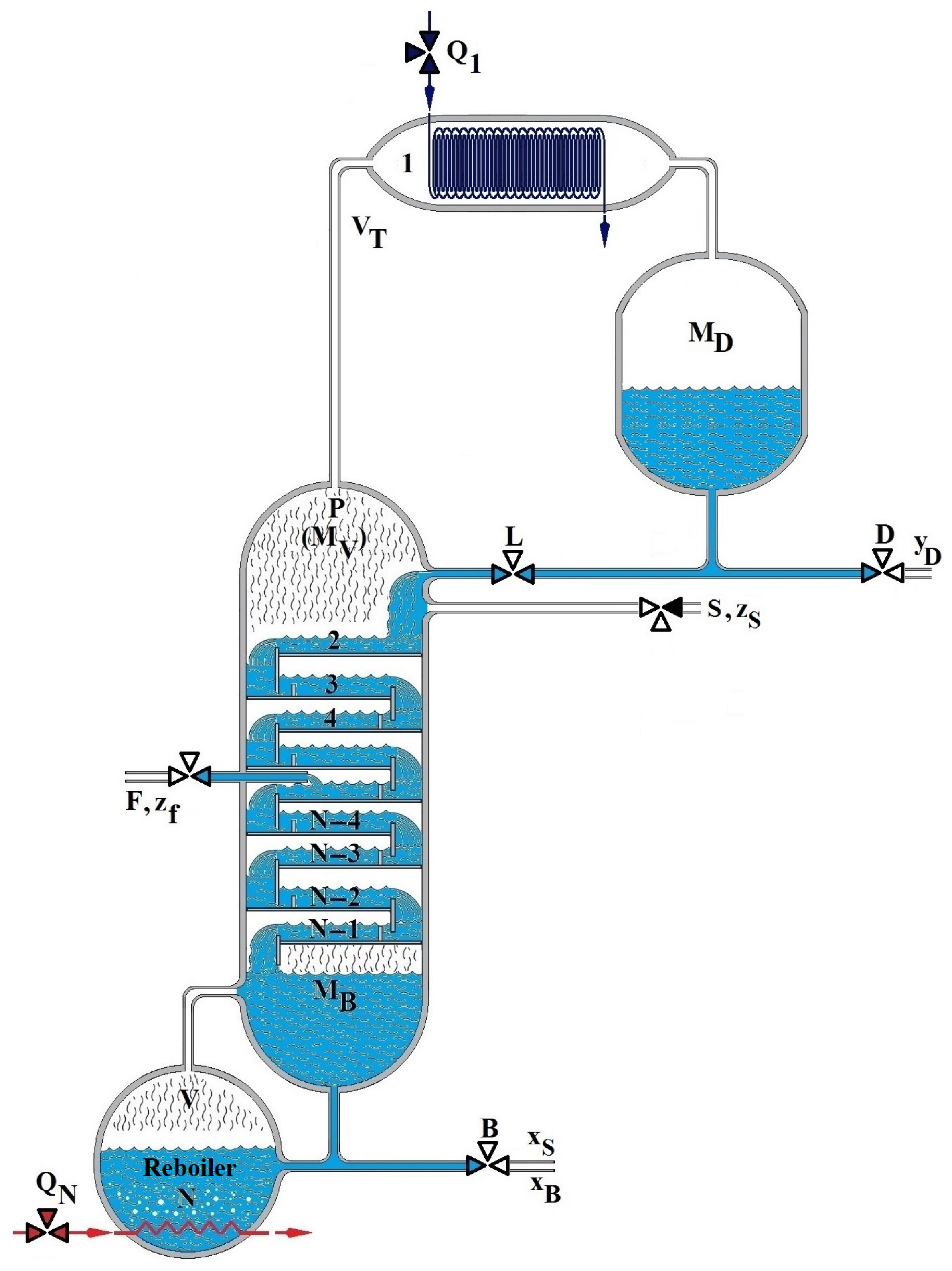
Description of the Extractive Distillation Column with Salt

Extractive distillation using salt as a separating agent operates on the same principle as conventional distillation. The main difference that exists is an extractive distillation column has a second feed typically located in the second tray of the column, and this is where the salt is introduced. This salt can be fed in solid form; however, it is not recommended because the salt can clog the feeding pipe; for this reason, it is recommended to dilute the salt with the reflux. In one way or another, the salt in each tray within the distillation column associates with the ethanol-water mixture creating the salting out effect. This effect is a phenomenon that consists in modifying the thermodynamic behavior of a mixture consisting of a solute in the aqueous phase by adding salt [38,39,40].

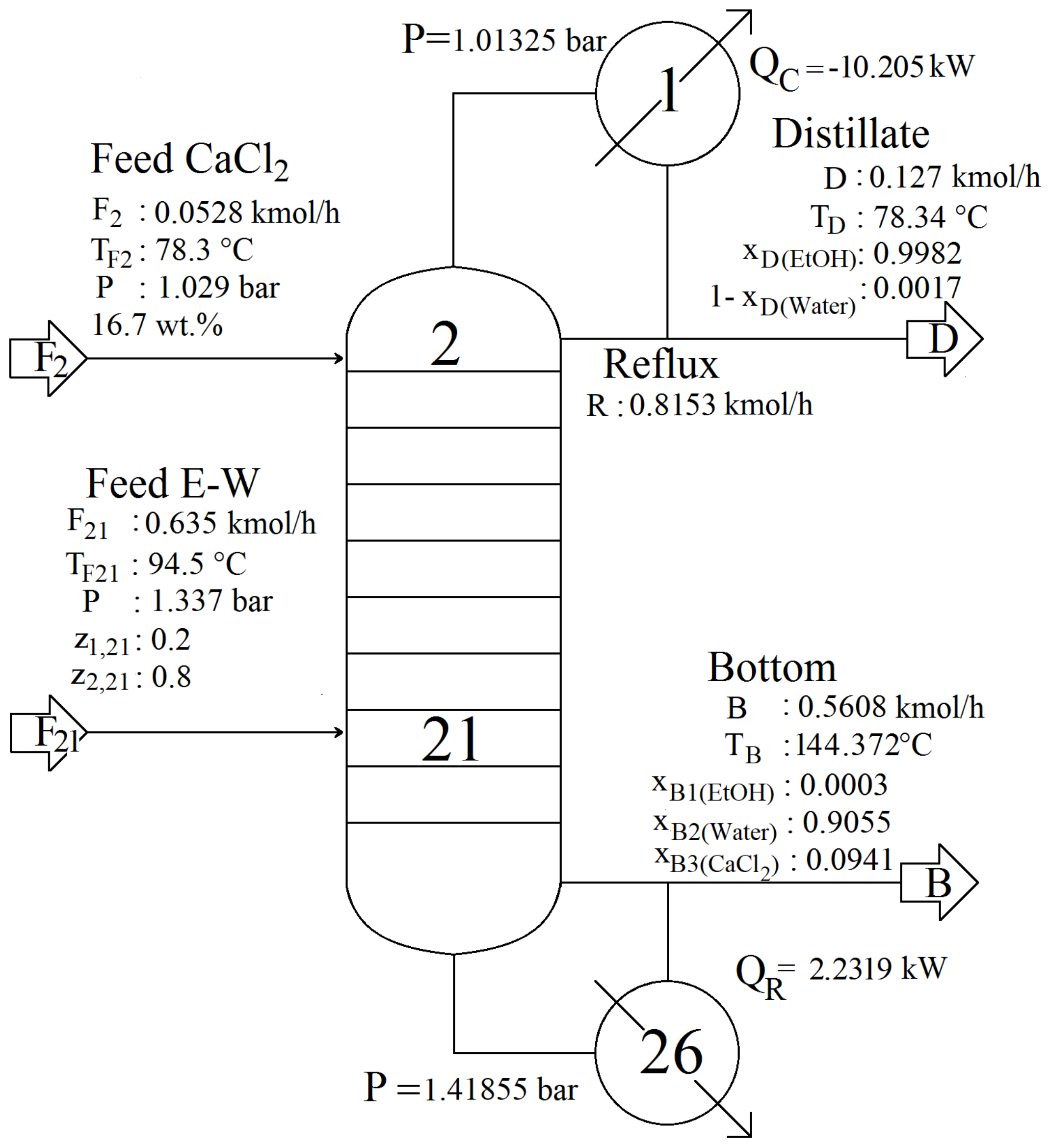
In the case of our column, the feed of the ethanol-water mixture enters as saturated vapor; in addition, there is a reflux current, through which the salt is also fed, whose compositions for the conditions described in

Table 1. Input data, specified parameters, and overall output data for the simulation of the saline extractive distillation column with CaCl${}_2$ as a separating agent.

Input/Output Data and Specified Parameters	Symbol	Value
Input data and specified parameters
Number of equilibrium stages	N	26
Main feed stage		21
Column efficiency (%)		50
Main feed thermodynamic state		Saturated vapor
Main feed temperature (${}^{°}$C)	T${}_{F,2}$	94.5
Main feed molar flow rate (kmol/h)	F${}_{21}$	0.635
Main feed ethanol mole fraction	x${}_{1,21}$	0.2
Main feed water mole fraction	x${}_{2,21}$	0.8
Salt feed molar flow rate (kmol/h)	F${}_2$	0.528
Salt feed temperature (${}^{°}$C)	T${}_{F,2}$	78.3
Distillate molar flow rate (kmol/h)		0.127
Reflux ratio		6.42
Operating pressure (atm)	P	1
Output data
Ethanol molar flow rate in distillate (kmol/h)	x${}_{1,1}$	0.127
Water molar flow rate in distillate (kmol/h)	x${}_{2,1}$	0.0017
Condenser heat duty (kW)	Q${}_C$	−10.205
Reboiler heat duty (kW)	Q${}_R$	2.2319

are x${}_3$ = 0.0648 on a free salt basis. This salt composition was calculated using Equation (4):

$$F_s=0.0648\times L\times F\times z$$

(4)

where 0.0648 is the composition of the salt; L is the reflux; F is the mixed feed; and z is the ethanol concentration.

Figure 1 shows the diagram of the column used in the simulation of extractive distillation of the ethanol-water-CaCl${}_2$ system, ready to incorporate the control loops (or control structures) and be evaluated. Table 1 summarizes the characteristics of the said plant; it has to produce ethanol above 99% mol of purity.

3. Simulation of Extractive Distillation Column with Salt in Stable State

The study that was taken as a basis to develop this simulation was the one developed by Llano-Restrepo et al. [16]. Who simulated the process in a stable state in the “FORTRAN” programming language with the thermodynamic model E-NRTL of absolute ethanol production at atmospheric pressure extractive distillation with the addition of 16.7 wt of CaCl${}_2$.

Unlike the study carried out by Llano-Restrepo et al. [16], in this work, the extractive distillation column was designed, simulated, and controlled at the pilot plant level using the Aspen Plus^® v8.6 simulator and the E-NRTL thermodynamic model, useful for predicting the VLE of an azeotropic mixture.

The simulation of the technique used includes the prediction of VLE-CaCl${}_2$, which was compared with the experimental data provided by Nishi [32]. To make this comparison, the activity coefficients had to be estimated in the E-NRTL thermodynamic model of the ethanol-water-CaCl${}_2$ system using the Aspen Properties^® DRS, since Aspen Plus^® does not have all.

Table 2. VLE data estimated from experimental data of the ethanol-water-CaCl${}_2$ system at 1 atm pressure and 16.7 wt% of CaCl${}_2$. Liquid phase apparent mole fractions: (a) ethanol; (b) water; (c) CaCl${}_2$; vapor phase mole fraction: (d) ethanol; (e) water; (f) temperatures.

(a)			(b)			(c)
${\mathit{x}}_{{\mathit{E}}_{\mathit{exp}}}$	${\mathit{x}}_{{\mathit{E}}_{\mathit{Est}}}$	$\Delta {\mathit{x}}_{\mathit{E}}$	${\mathit{x}}_{{\mathit{W}}_{\mathit{exp}}}$	${\mathit{x}}_{{\mathit{W}}_{\mathit{Est}}}$	$\Delta {\mathit{x}}_{\mathit{E}}$	${\mathit{x}}_{{{\mathit{CaCl}}_{\mathit{2}}}_{\mathit{exp}}}$	${\mathit{x}}_{{{\mathit{CaCl}}_{\mathit{2}}}_{\mathit{Est}}}$	$\Delta {\mathit{x}}_{{\mathit{CaCl}}_{\mathit{2}}}$
0	0	0	0.9736	0.9736	0	0.0264	0.0264	0
0.0195	0.0195	0	0.9534	0.9534	0	0.0271	0.0271	0
0.0389	0.0389	0	0.9331	0.9331	0	0.028	0.028	0
0.097	0.097	0	0.8727	0.8727	0	0.0303	0.0303	0
0.1931	0.1931	0	0.7725	0.7725	0	0.0344	0.0344	0
0.2885	0.2885	0	0.6732	0.6732	0	0.0383	0.0383	0
0.3831	0.3831	0	0.5747	0.5747	0	0.0422	0.0422	0
0.477	0.477	0	0.477	0.477	0	0.046	0.046	0
0.5701	0.5701	0	0.3801	0.3801	0	0.0498	0.0498	0
0.6625	0.6625	0	0.2839	0.2839	0	0.0536	0.0536	0
0.7541	0.7541	0	0.1885	0.1885	0	0.0574	0.0574	0
0.845	0.845	0	0.0939	0.0939	0	0.0611	0.0611	0
0.9352	0.9352	0	0	0	0	0.0648	0.0648	0
(d)			(e)			(f)
${\mathit{y}}_{{\mathit{E}}_{\mathit{exp}}}$	${\mathit{y}}_{{\mathit{E}}_{\mathit{Est}}}$	$\Delta {\mathit{y}}_{\mathit{E}}$	${\mathit{y}}_{{\mathit{W}}_{\mathit{exp}}}$	${\mathit{y}}_{{\mathit{W}}_{\mathit{Est}}}$	$\Delta {\mathit{y}}_{\mathit{W}}$	${\mathit{T}}_{\mathit{exp}}$	${\mathit{T}}_{\mathit{Est}}$	$\Delta {\mathit{T}}_{{}^{°}\mathit{C}}$
0	0	0	1	1	0	102.8	104.51	1.7116
0.271	0.2710	6.90 × ${10}^{-6}$	0.729	0.7634	0.0344	96.00	97.737	1.7370
0.389	0.3890	2.49 × ${10}^{-6}$	0.611	0.5872	0.0237	91.60	91.329	0.2709
0.542	0.5420	2.41 × ${10}^{-6}$	0.458	0.4150	0.0429	85.00	84.293	0.7061
0.647	0.6470	3.13 × ${10}^{-7}$	0.353	0.3439	0.0090	82.45	82.334	0.1158
0.694	0.6940	1.25 × ${10}^{-7}$	0.306	0.3003	0.0056	81.45	81.800	0.3500
0.753	0.7529	4.70 × ${10}^{-7}$	0.247	0.2686	0.0216	81.25	82.396	1.1466
0.795	0.7949	4.16 × ${10}^{-7}$	0.205	0.2276	0.0226	80.70	82.383	1.6831
0.828	0.8279	1.41 × ${10}^{-7}$	0.172	0.1819	0.0099	81.50	82.027	0.5274
0.867	0.8669	4.02 × ${10}^{-8}$	0.133	0.1360	0.0030	81.50	81.788	0.2887
0.915	0.9150	7.86 × ${10}^{-9}$	0.085	0.0904	0.0054	82.40	81.743	0.6561
0.942	0.9420	8.14 × ${10}^{-8}$	0.058	0.0438	0.0141	81.65	81.045	0.6044
1	1	0	0	0	0	82.65	81.123	1.5263

shows the results and the differences ($\Delta$) of the compositions in apparent and salt-free molar fractions of the experimental data and those estimated by the DRS.

Table 3. Comparison between the data calculated by the $DRS$ versus the experimental data of Nishi and those estimated by Llano and Hashemi: (a) vapor phase; (b) differences between the vapor phase data; (c) temperatures; (d) difference between the temperature data.

(a)					(b)
Nishi		$\mathit{DRS}$	Llano	Hashemi	$\Delta {\mathit{y}}_{\mathit{Exp}}$
${\mathit{x}}_{\mathit{Exp}}$	${\mathit{y}}_{\mathit{Exp}}$	${\mathit{y}}_{\mathit{Est}}$	${\mathit{y}}_{\mathit{Est}}$	${\mathit{y}}_{\mathit{Est}}$	$\mathit{DRS}$	$\mathit{Llano}$	$\mathit{Hashemi}$
0	0	0	0	0	0	0	0
0.02	0.271	0.271	0.264	0.271	0	0.007	0
0.04	0.389	0.389	0.394	0.393	0	0.005	0.004
0.10	0.542	0.542	0.558	0.466	0	0.016	0.076
0.20	0.647	0.647	0.651	0.595	0	0.004	0.052
0.30	0.694	0.694	0.701	0.694	0	0.007	0
0.40	0.753	0.753	0.743	0.762	0	0.010	0.009
0.50	0.795	0.795	0.785	0.800	0	0.010	0.005
0.60	0.828	0.828	0.829	0.840	0	0.001	0.012
0.70	0.867	0.867	0.872	0.868	0	0.005	0.001
0.80	0.915	0.915	0.916	0.910	0	0.001	0.005
0.90	0.942	0.942	0.959	0.941	0	0.017	0.001
(c)					(d)
Nishi	$\mathit{DRS}$	Llano	Hashemi		$\Delta \mathit{T}{}^{°}{\mathit{C}}_{\mathit{Exp}}$
${\mathit{T}}_{\mathit{Exp}}$	${\mathit{T}}_{\mathit{Est}}$	${\mathit{T}}_{\mathit{Est}}$	${\mathit{T}}_{\mathit{Est}}$		$\mathit{DRS}$	$\mathit{Llano}$	$\mathit{Hashemi}$
102.8	104.51	103.69	108.5		1.71	0.89	5.70
96.00	97.74	95.92	96.01		1.74	0.08	0.01
91.60	91.33	91.41	87.67		0.27	0.19	3.93
85.00	84.29	85.16	84.12		0.71	0.16	0.88
82.45	82.33	82.10	82.62		0.12	0.35	0.17
81.45	81.80	81.30	81.46		0.35	0.15	0.01
81.25	82.4	81.11	80.83		1.15	0.14	0.42
80.70	82.38	81.14	80.88		1.68	0.44	0.18
81.50	82.03	81.27	81.49		0.53	0.23	0.01
81.50	81.79	81.47	81.84		0.29	0.03	0.34
82.40	81.74	81.72	82.43		0.66	0.68	0.03
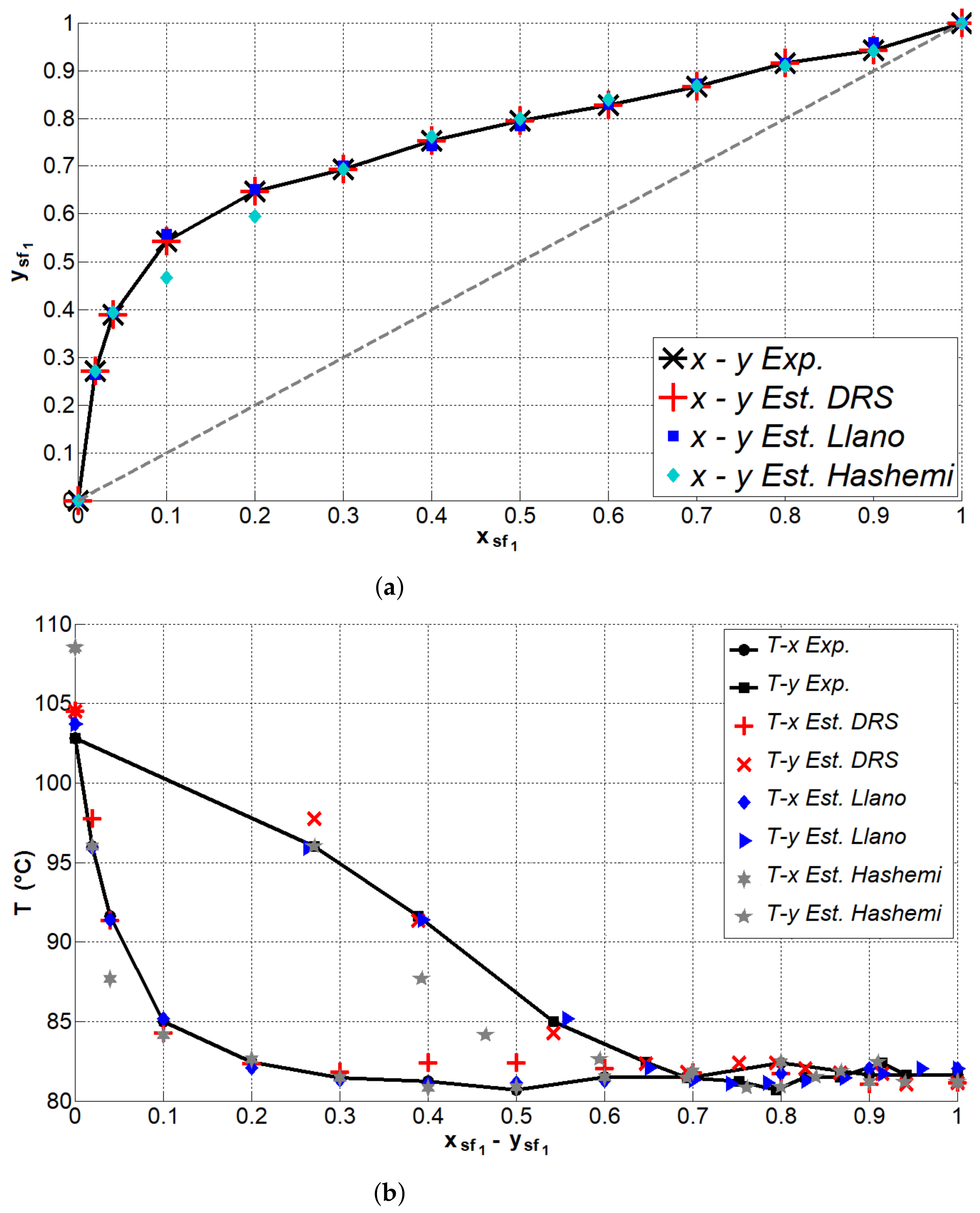
81.65	81.05	82.02	81.19		0.60	0.37	0.46

shows and compares the data reported in the literature for VLE-CaCl${}_2$. Experimental data were reported by Nishi (1975) [32]; Llano-Restrepo et al. [16]; and Hashemi et al. [33] vs. Aspen Plus^® DRS estimates. It is worth mentioning that only the vapor phase ($y_{Exp,Est}$) was reported, since it is the most important product to be obtained in the distillation, in addition to the absence of salt. In Figure 2, these data are represented graphically. It can be seen that the data regressed by the DRS in the vapor phase are very good approximations with respect to the experimental and temperature data; it can be seen that at the bottom of the equilibrium, the data estimated by the DRS have a maximum error of 1.74 ${}^{°}$C. This bottom of the equilibrium represents the reboiler of the extractive distillation column.

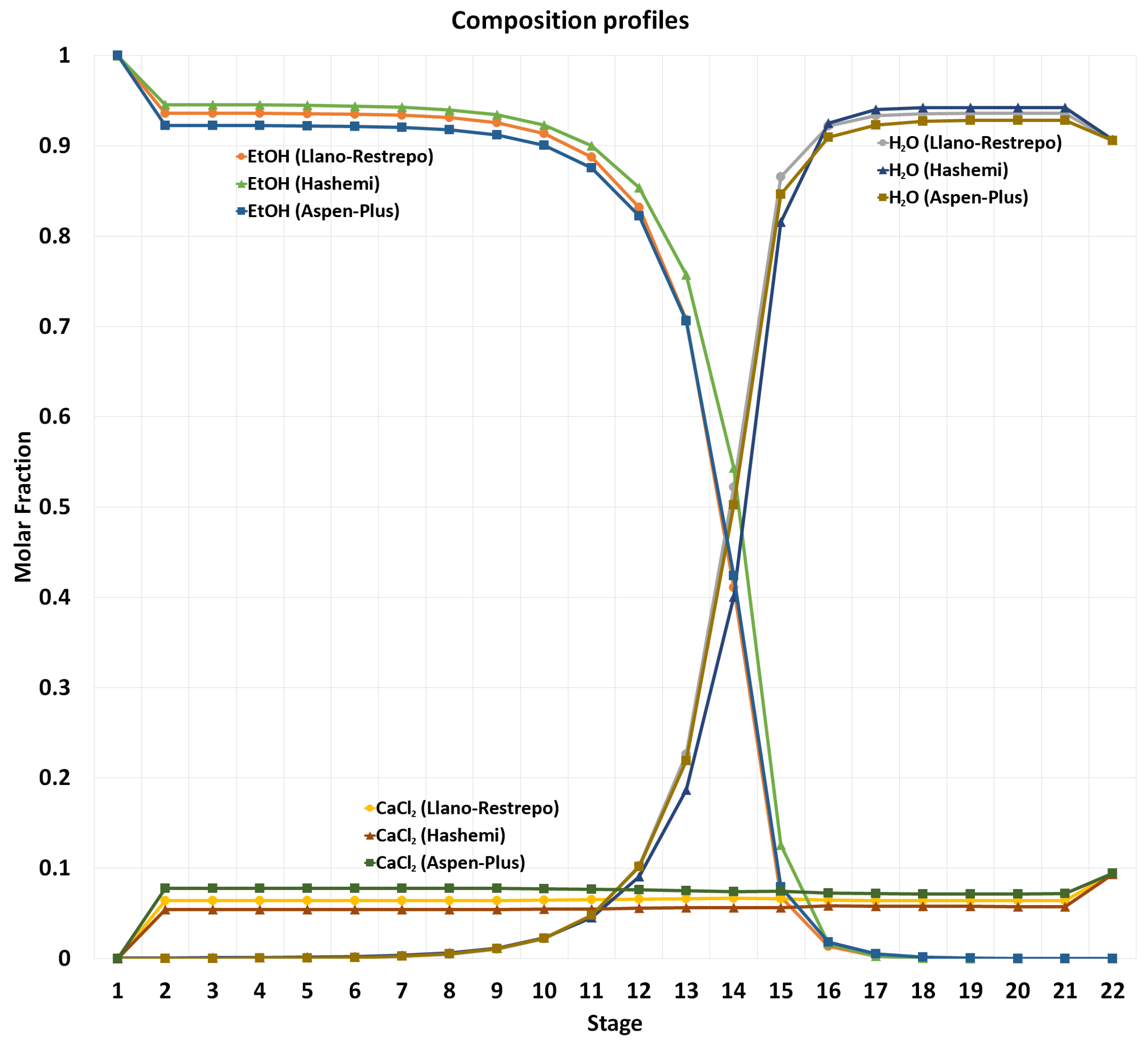
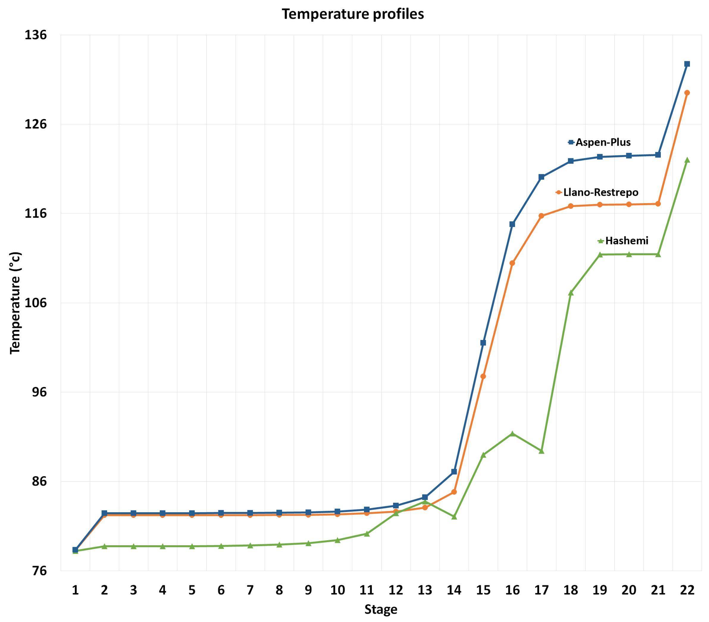
In addition, the extractive distillation simulation was performed using the Aspen Plus^® RadFrac block, which performs rigorous calculations for columns in ordinary distillation, extractive distillation applications, and more; solving the MESH equations. Figure 3 shows the graph of the composition profile results and Figure 4 shows the graph of the simulation temperature results. These profiles were analyzed and compared with the results reported in [16,33], obtaining a relative error of less than 5%.

When the results of the VLE-CaCl${}_2$ and the profiles of the salt distillation column were compared and validated, the next step was to design our own extractive salt distillation column using RadFrac tool of Aspen Plus^®, in order to add dynamics to our plant.

4. Dynamic Simulation of Extractive Distillation Column with Salt

Dynamic simulation is used to evaluate control strategies in the face of disturbances. To perform the dynamics of the simulation carried out in Aspen plus^® v8.6, it had to be exported to Aspen Plus Dynamics^® v8.4 using the “pressure-driven” option. Before exporting it, it was necessary to size the equipment. For this, the procedure proposed in the book by Treybal [41] was used and compared with the application of tray-sizing of the RadFrac block of Aspen Plus^®. This application calculates the characteristics of the distillation column. The levels of the reflux tanks and the one at the base of the column were calculated using the method proposed by Luyben [42] proposing 10 min of retention or hold up when they are at 50% of the liquid level.

Table 4. Characteristics of the column of the saline extractive distillation column.

Characteristics	Aspen Plus®	Treybal	Luyben
Number of stages	24	24	24
Tray spacing (m)	0.10	0.15	N.A.
Flooding factor ($C_f$)	0.80	0.0424	N.A.
Foaming factor	0.80	0.80	N.A.
Column diameter (m)	0.102	0.11	0.10
Total area (m${}^2$)	0.0081	0.0095	0.0077
Active area per panel (m${}^2$)	0.0065	0.0062	N.A.
Downcomer area (m${}^2$)	0.000816	0.00083	N.A.
Weir height (m)	0.074	0.077	N.A.
Reflux drum total liquid volume (L)	N.A.	N.A.	10
Reboiler total liquid volume (L)	N.A.	N.A.	2
N.A. = Not Applicable

shows the characteristics obtained by these methods. It should be noted that the total number of trays reported in Table 4 does not consider tray number 1 and the last tray, since they are the condenser and the reboiler, respectively.

Aspen Plus Dynamics^® simulations use rigorous nonlinear models. The E-NRTL thermodynamic model was used due to its ability to closely match the ethanol-water-CaCl${}_2$ VLE experimental data. The column operates at 1 atmospheric pressure with a pressure drop of 0.016 atm per tray. The feed flow rate is 0.635 kmol/h. Aspen^® tray numbering notation is used (numbered stages from reflux drum to kettle). Total condensers, partial reboilers, and trays with efficiencies of 50% are used to try to make it as real as possible, these efficiencies were estimated from the O’Connell empirical correlation. A column that produces high-purity products at both ends was considered in this article.

4.1. Analysis and Location of Temperature Sensing

In the distillation columns, the compositions are measured directly by composition analyzers by means of chromatography; however, this implies a dead time of 5 to 10 min, also, its reliability is insufficient for online control. Another way to infer its composition is from temperature measurements on the trays, as this is less expensive and faster for indirect composition control, plus it usually has a lag time constant that will depend on the specifications of the sensor to use.

In distillation columns with binary isobaric systems (constant pressure), the temperature is relative to the composition. In other words, temperature measurements provide accurate information on component concentrations; however, they must be strategically located on the column tray(s). This will depend on the products or degrees of freedom that we want to control within the salt extractive distillation column.

Thanks to temperature sensors, it is possible to effectively control its composition. Furthermore, such sensors are inexpensive and reliable, and introduce only a small measure of delay to the control loop. Therefore, temperature measurements are widely used to provide inferential control of compositions [43].

The selection of the tray to control its temperature (this is the reference to infer the concentration) is not usually a matter of dynamics but changes in the stable state; for this, a balance must be maintained between the following two rules:

• The temperature of the tray must be insensitive to changes in the composition of the feed, in other words, the composition must be constant.
• The temperature of the tray must be sensitive to changes in the manipulated variable.

The balance of these two rules can be conducted using different selection criteria. The three criteria used in this work are described in more detail in Luyben [44].

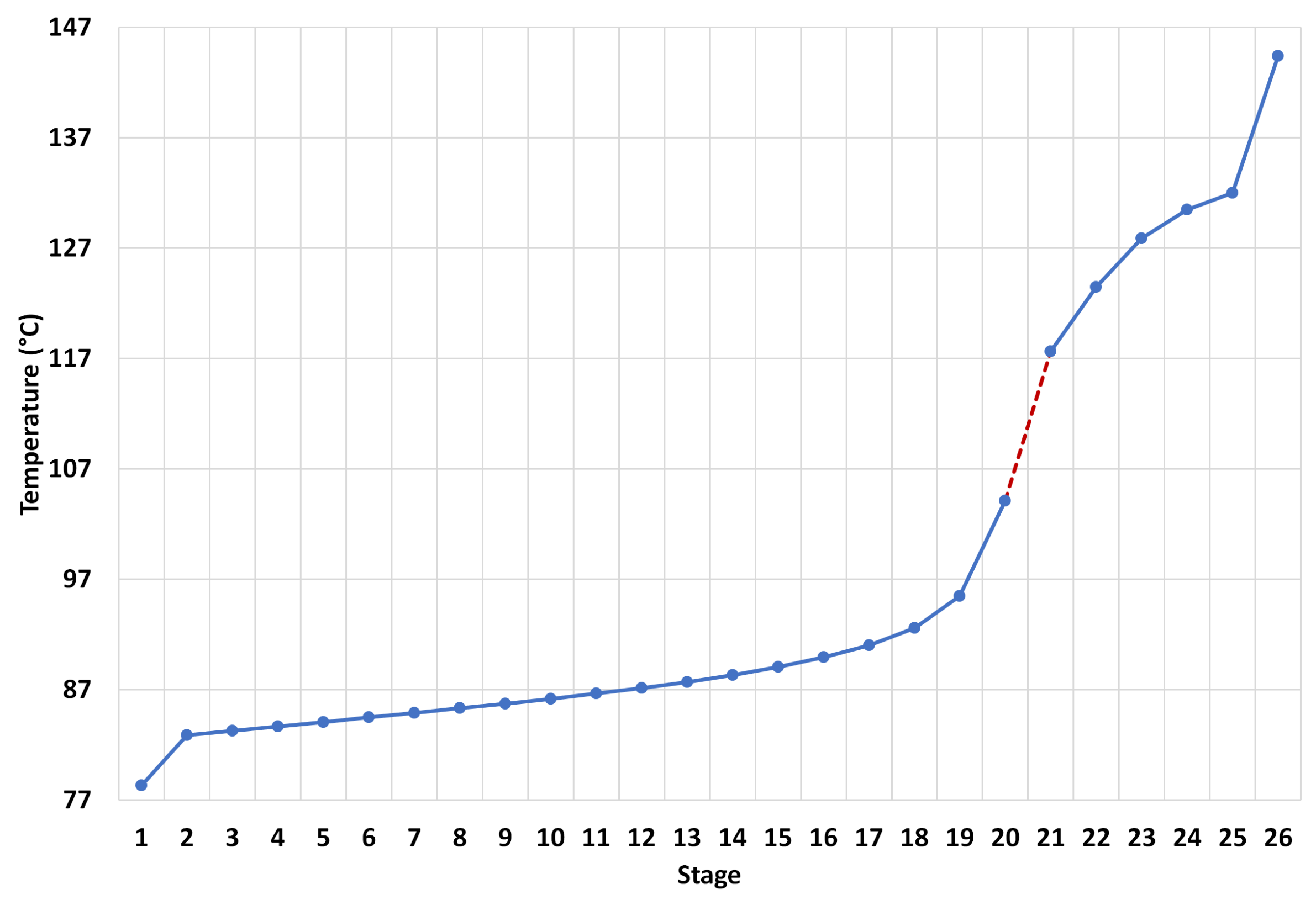
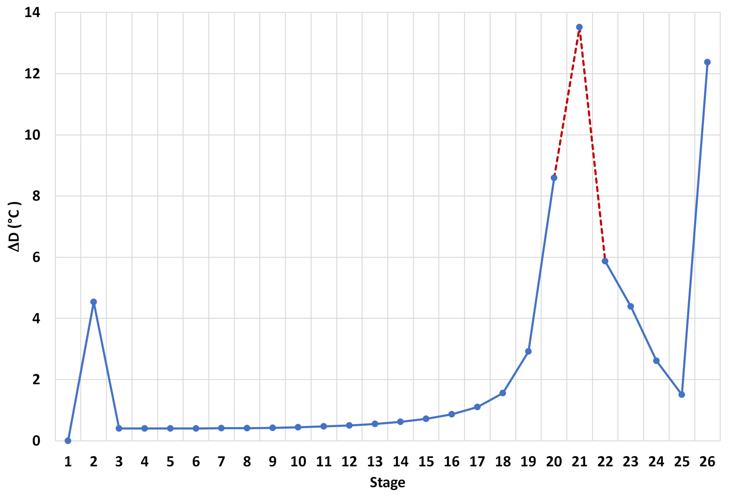
The first criterion used was the maximum slope criterion in the temperature profile. The development was as follows:

• From the results of the temperature profile of the simulation in the steady state with its nominal inputs, the tray or the stage of the temperature profile that varies the most in the column must be selected. This tray or stage of the column is the location where the temperature must be measured by a sensor.
• Figure 5 deals with the temperature profile of the ethanol-water-CaCl${}_2$ column simulation. In Figure 6, small temperature variations are observed from the top to stage 17; therefore, stages 20 and 22 were selected because they have the maximum slopes.

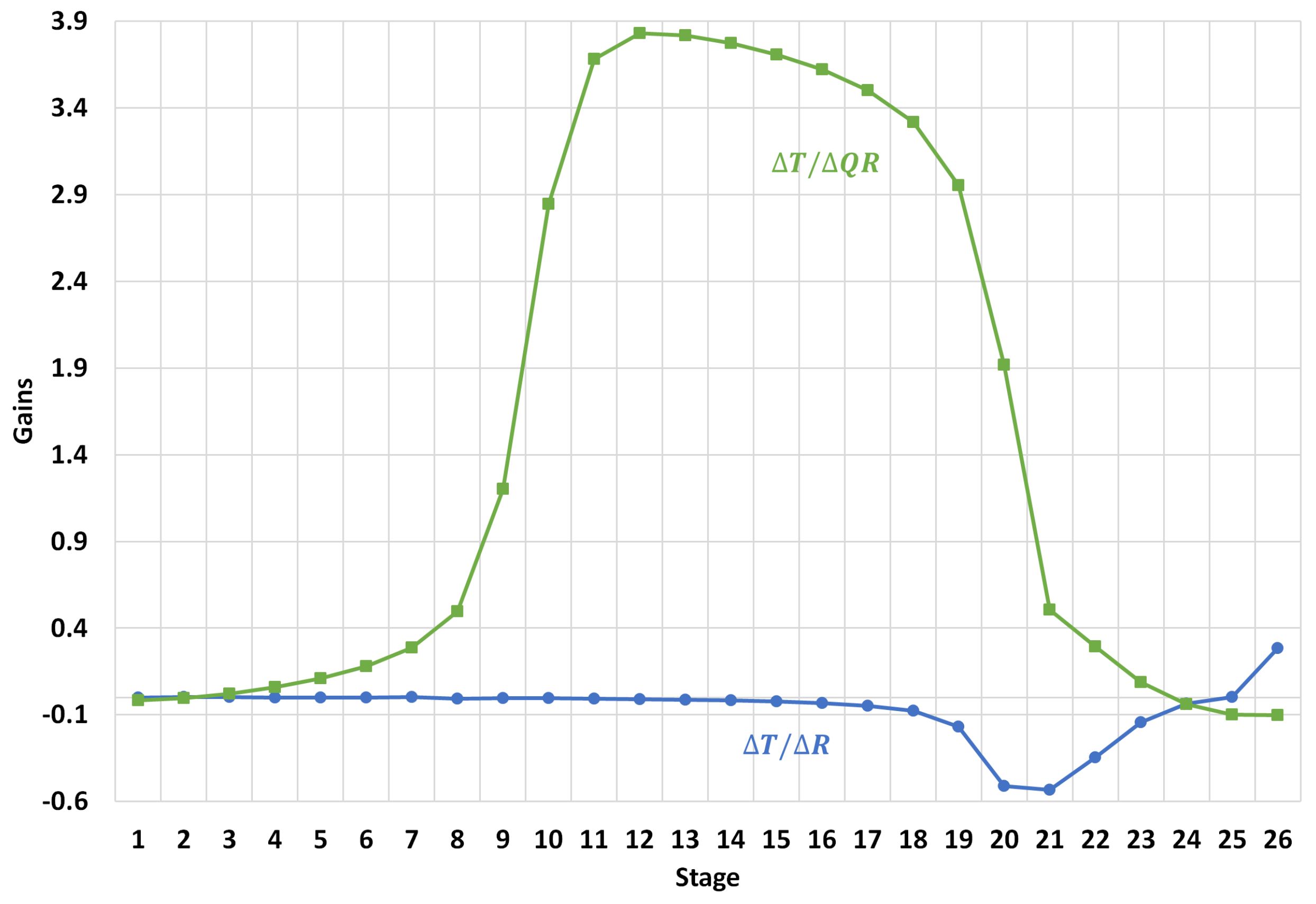
The second criterion used was sensitivity. Its development is described below:

• A small change in the manipulated variables must be made to analyze the changes in temperature, stage by stage.
• For a $dualend$ control strategy, it is necessary to measure the influence that exists on the temperature when making a small change in reflux (L) and heat in the reboiler (V).
• Therefore, a small change in the reboiler heat and reflux (0.3% and 3%, respectively) is introduced and the variation in the temperature profile is analyzed. Figure 7 shows the results of the analysis of the gain matrix $K_{26\times 2}$ and as can be seen, stage 20 is more affected by changes in reflux than the rest of the column. On the other hand, between stages 18 and 22, it is affected more by changes in the reboiler heat, and stage 22 is selected because it is below the feed.

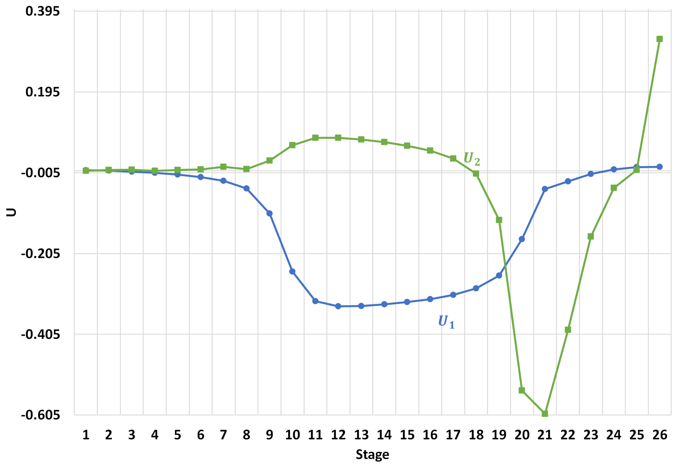
The third criterion was the SVD criterion.

• The gain matrix K was factored into three matrices: K = USV, where K and U obtain information on the sensitivity and interaction of the sensors Figure 8. The absolute maximum value of vector U${}_1$ shows the location of the most temperature-sensitive sensor, while the second position, vector U${}_2$, indicates less interaction (sensitivity) with respect to the first position, Luyben (2012). In the case of the ethanol-water-CaCl${}_2$ distillation, the simulations indicate that the appropriate location of the sensors above the main feed inlet (which corresponds to the largest value of the vector U${}_1$) is stage 20 and below the main feed input is stage 22 (maximum value of the vector U${}_2$). The results for the $dualend$ control are shown in Table 2.

Figure 8. Singular value decomposition (SVD). Analysis of singular vectors U${}_1$ and U${}_2$ vs. stage location.

Figure 8. Singular value decomposition (SVD). Analysis of singular vectors U${}_1$ and U${}_2$ vs. stage location.

In summary, the manipulation of the temperatures of trays 20 and 22 for the use of the structure of two control points, was the result of the application of the three criteria described above, taking into account that, in reality, the trays of the column are not affected immediately by either temperature or changes in the reflux flow. For this reason, in the simulation with Aspen Dynamics^®, a delay of 6 s per tray is considered, giving a total of 2 min on the tray 20 control loop sensor, while a delay of 2.2 min was placed on the tray 22 sensor [42,44,45,46,47].

Disturbances

Disturbances are random alterations that affect our main system or plant variables. In the case of the extractive distillation column, the main feed flow (F) can be considered as a disturbance since it has a composition ($z_F$) and a condition ($q_f$, steam). This flow is considered a disturbance because it affects the four output variables of the column ($y_D$, $x_B$, $M_B$, $M_D$). Furthermore, according to Luyben [48], variations in the composition of the feed are the main disturbances that exist in the control of a distillation column.

On the other hand, Figure 9 shows the extractive distillation column and its variables, the salt feed flow (S or $F_S$), which also has a composition ($z_S$) and a condition ($q_S$, solid); it is not considered a disturbance because this flow does not disturb or affect the distillation column, as when it varies or there are changes in the main feed, whether in flow, composition, or reflux ratio, this feed also changes. That is why this feed flow (S) is considered an ideal control and has a relationship through Equation (4).

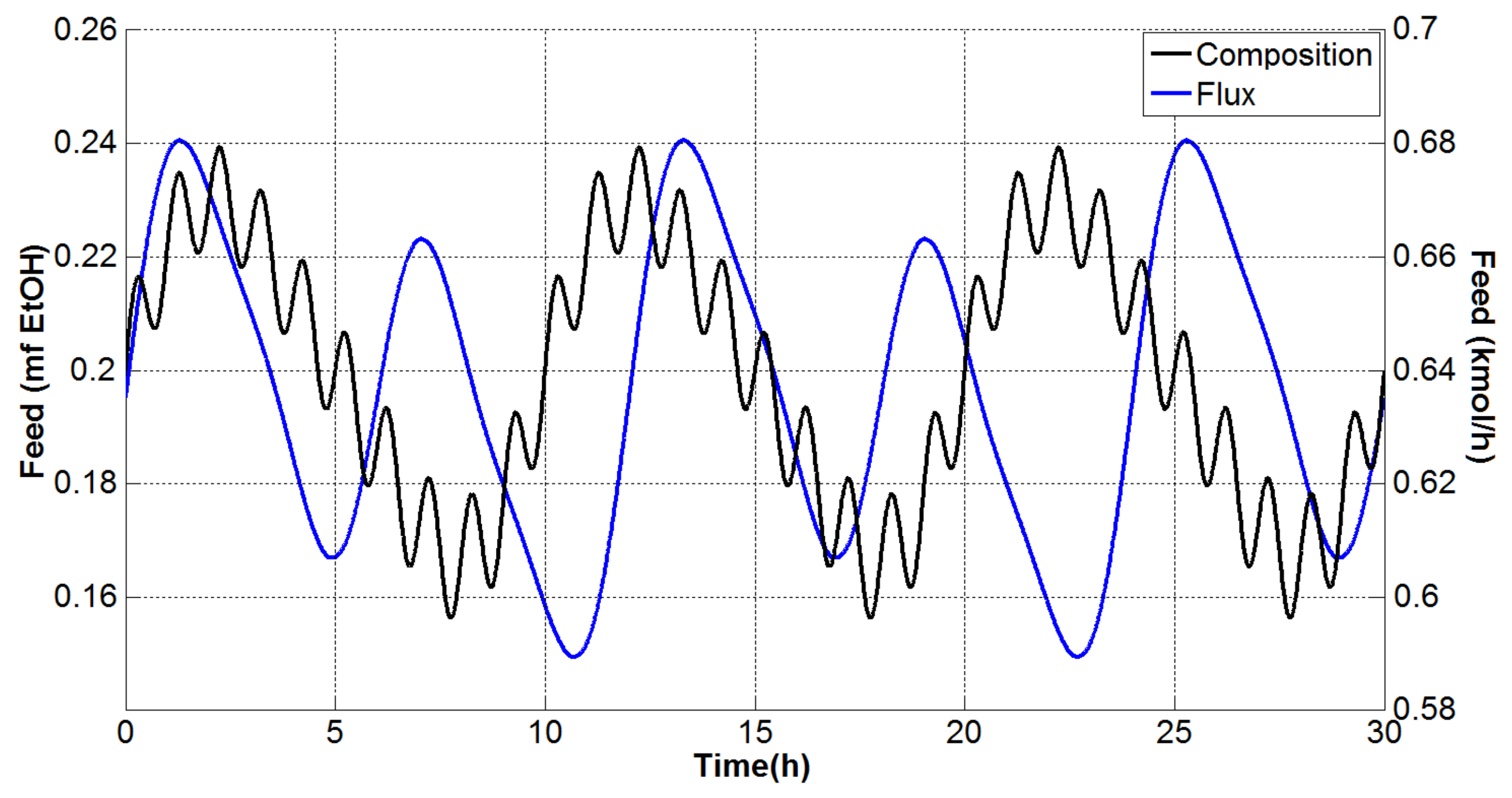
Figure 10 shows the continuous fluctuation disturbance. This perturbation is one of two perturbations used to evaluate the control structures.

This fluctuation was the result of the sum of three sinusoidal functions with different frequencies. The first simulations were performed with a +10% change in the composition of the ethanol in the input feed, then, a change of −10% was considered. The second series of tests was carried out in the same way but altered the nominal flow of the feed. As mentioned at the beginning of this paragraph, the third series of tests used continuous fluctuations; combining the oscillations in the feed flow and the composition of the ethanol, the different series of perturbations were introduced individually to analyze their behavior.

5. Control Strategy

In industrial practice, it is important to choose the right control structure for a distillation column. There is no “unique” structure for all columns, so some authors consider that each column should be treated independently [49]. As mentioned above, the development of the control strategy requires the conversion of the steady state model to a dynamic model to evaluate the effect of the main disturbances in the extractive distillation column.

Within the control strategies for conventional distillation columns, the control of one or two main variables is considered and this will depend on: (1) alterations in the composition of the feed and the final products; and (2) power consumption. These two types of controls were considered for the saline extractive distillation column since, as mentioned above, the extractive distillation column contains an ideal control by means of the relation of the Equation (4); therefore, the modeling of the saline extractive distillation column was treated as a binary distillation column because it considered a mixture of two pseudo-components: ethanol/salt—Water/salt. The input variables, also called manipulated variables (u) of the said column, are: reflux (L); the distillate (D); the heat in the reboiler ($Q_N$ or V); the heat removed from the condenser ($Q_1$ or $V_T$); and the bottom current (B). The output variables (y) or controlled variables are the distillate ($y_D$) and residue ($x_B$) products; as well as the levels in the reflux tanks ($M_D$), column base ($M_B$), and pressure (P or $M_V$), and can be seen in Figure 9. Consequently, the control for this distillation column is posed as a problem of $5\times 5$ [50] (see Equation (5)).

$$u=\left(\begin{array}{c}L\\ D\\ B\\ Q_1\\ Q_N\end{array}\right);y=\left(\begin{array}{c}{y}_D\\ x_B\\ M_D\\ M_B\\ P\end{array}\right)$$

(5)

The output variables $M_D$, $M_B$, and P, are part of the secondary control loops, which ensure stability and operability in the process. This problem can be reduced to one of the following two options:

(i)

Control of a primary loop or $1\times 1$. This type of control is used when there is a mixture of two components and the interest is to maintain the purity of a product or a column stream. This structure is called the $singleend$ or $singlepointcontrol$. The variables to manipulate for this work were L and D.

(ii)

Control of two primary loops or $2\times 2$. This type of control is used when there is a mixture of more than two components whose objective is to preserve the purity close to the desired specifications in the two product streams of the distillation column, both the distillate and the bottom [51]. Therefore, the structure called $dualend$ is used. These control loops define and give the name to the control structure or strategy. The basic control structures to be used in this work are LV and DV.

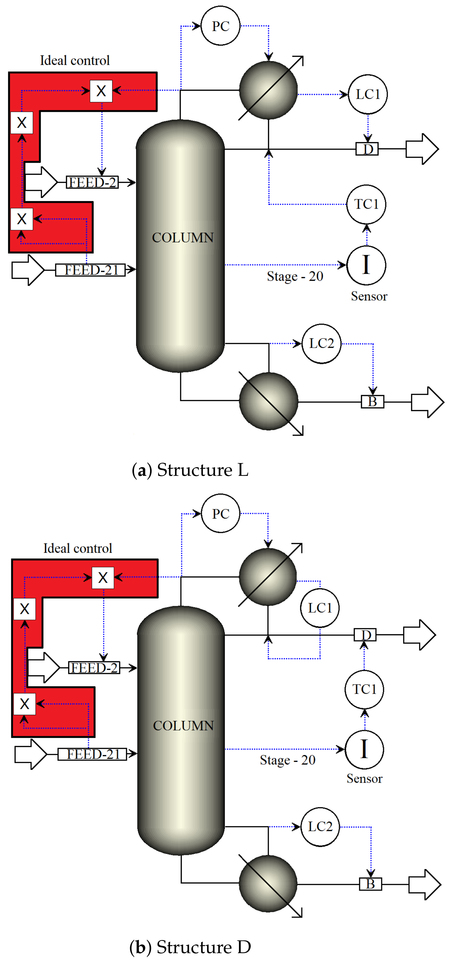
5.1. Single End Structures

To evaluate the behavior of the column before the aforementioned disturbances, it was necessary to install the following control loops for structure L (Figure 11a):

• Loop TC1: The temperature controller on tray 20. The flow rate of the reflux is used to regulate the temperature of this tray.
• PC loop: Pressure controller. The condenser pressure is controlled by manipulating the flow of liquid from the condenser.
• Loop LC1: Reflux tank level controller. The level of the reflux tank is regulated by manipulating the flow of the distillate.
• Loop LC2: Waste tank level controller. The bottom tank level of the column is regulated by manipulating the flow of the residue.
• FEED-2 loop: CaCl${}_2$ feed. The salt feed is controlled by an ideal flow controller in order to fix the salt concentration close to 16.7 p/p in all of the trays of the column (to preserve the validity of the ELV estimate). The salt feed flow is calculated online using Equation (4).

Moreover, for structure D (Figure 11b), the control loops are the same, unlike loop TC1; temperature controller on tray 20. To regulate the temperature in this tray, the distillate flow is used.

The gains of the four controllers that were used in the simulation of the structures in Figure 11a,b are reported in

Table 5. Controller gain for the single temperature control.

(a) Structure L						(b) Structure D
Controller		PC	LC1	LC2	TC1	Controller		PC	LC1	LC2	TC1
P	$K_C$	17.8	26.01	32.6	1.44	P	$K_C$	17.8	87.8	32.6	2.15
I	${\tau }_I$	1.5	7	1	12.6	I	${\tau }_I$	1.5	2.5	1	26.1
D	${\tau }_D$				3.15	D	${\tau }_D$				6.52

, of which, the secondary loops are PIs and the main loop (the temperature one) is PID. The tunings were performed using the Ziegler-Nichols oscillation method.

5.2. Dual End Structures

For structures with two control points, the problem to be solved is the adjustment or control of the temperatures, since there is an interaction between the two loops. However, the condition number (CN) calculated from $SVD$ of the general gain matrix G (Figure 8), suggests that the $controldual$ of the temperature is possible. Normally, this structure is recommended by Luyben [51]:

• For columns with medium and high concentration feeds;
• When the control cannot be resolved with a control $singleend$;
• When a high purity is required in both products (distillate and bottom).

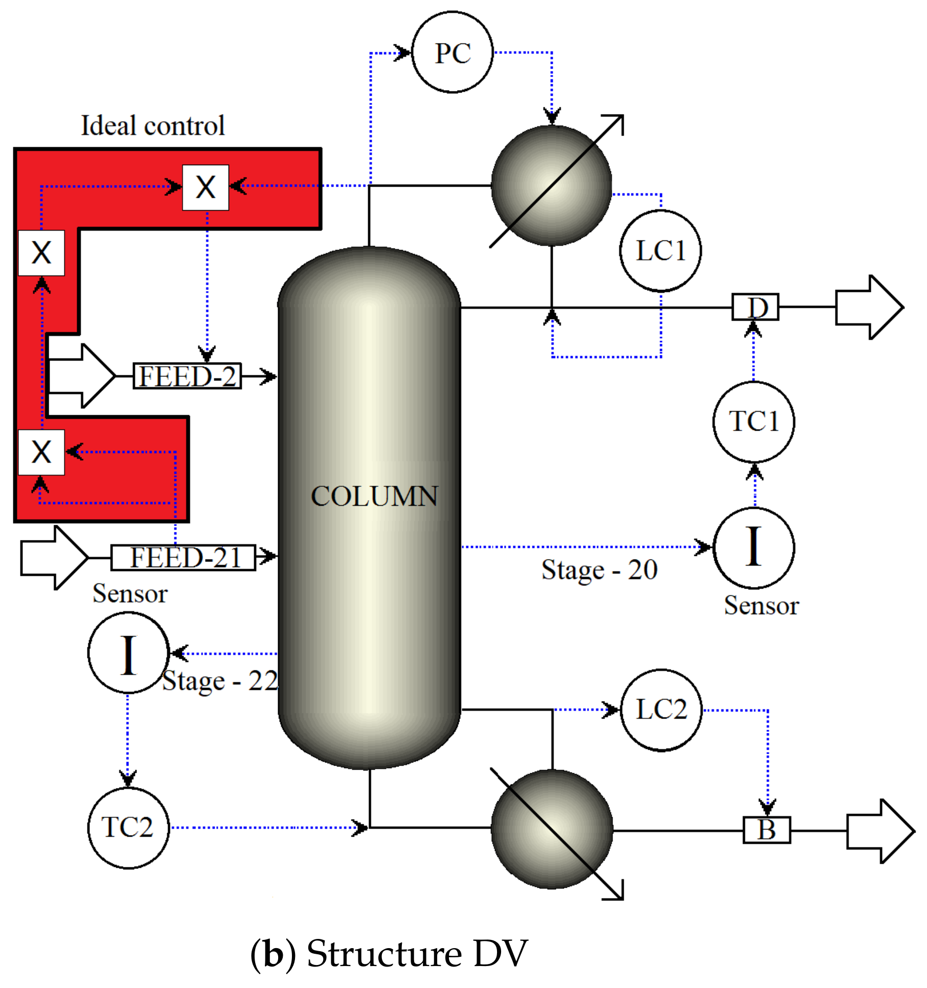
In Figure 12a, the $LV$ control structure is shown and the control loops are clearly seen, which are defined as follows:

• Loop TC1: Temperature controller on tray 20. The flow rate of the reflux is used to regulate the temperature of this tray.
• Loop TC2: Temperature controller in tray 22. The regulation of the temperature in this tray is conducted by means of the heat from the reboiler.
• PC loop: Pressure controller. Regulation of the flow of the liquid from the condenser controlled condenser pressure.
• Loop LC1: Reflux tank level controller. The level of the reflux tank is regulated by manipulating the flow of the distillate.
• Loop LC2: Waste tank level controller. The level at the bottom of the column is regulated by manipulating the bottom flow.
• FEED-2 loop: CaCl${}_2$ feed. The salt feed is controlled by an ideal flow controller, in order to fix the salt concentration close to 16.7 p/p in all the trays of the column (to preserve the validity of the ELV estimate). The salt feed flow is calculated online using Equation (4).

Likewise, the control loops for the $DV$ structure (Figure 12b) are the same, unlike the TC1 loop; temperature controller on tray 20. To regulate the temperature in this tray, the distillate flow is used.

The gains of the five controllers that were used in the simulation of the structures in Figure 12a,b are shown in

Table 6. Controller gain for the dual temperature control.

(a) Structure LV							(b) Structure DV
Controller		PC	LC1	LC2	TC1	TC2	Controller		PC	LC1	LC2	TC1	TC2
P	$K_C$	17.8	26.01	32.6	1.44	49.8	P	$K_C$	17.8	26.01	32.6	2.15	49.8
I	${\tau }_I$	1.5	7	1	12.6	4.5	I	${\tau }_I$	1.5	7	1	26.1	4.5
D	${\tau }_D$				3.15	1.12	D	${\tau }_D$				6.52	1.12

. Of which, the secondary loops are PIs and the main loops (the temperature ones) are PIDs. The tunings were performed using the Ziegler-Nichols oscillation method.

6. Checking and Assessment of Control Structures

The purpose is to comply with the international standard of ethanol purity; for this, it is necessary to adjust the temperature in one or two trays during the period of operation of the distillation column. For this reason, four control structures were designed and evaluated. This evaluation was carried out using common criteria, where the temperatures of the trays were measured to infer the concentration. These criteria are defined below:

• IAE (Integral absolute errors)—this criterion tells us how close the composition in the distillate maintains the desired purity. In other words, it shows the variation of the measured signal before a reference value.

  $$IAE={\int }_0^{\infty }\mid e\left(t\right)\mid dt$$

  (6)
• ISE (Error square integral)—this error is represented in time and indicates the errors that exist in relation to the reference; therefore, its value increases because the size of the error grows. This error does not capture small errors.

  $$ISE={\int }_0^{\infty }e{\left(t\right)}^{2}dt$$

  (7)
• ITAE (Integral absolute error multiplied by time)—the result is defined over the duration of the simulation. Large values of this error are interpreted as fluctuations in the system; as shown in the simulations, disturbances in the composition of the feed cause an oscillation at the limits of a new steady state.

  $$ITAE={\int }_0^{\infty }t\mid e\left(t\right)\mid dt$$

  (8)
  This ITAE is defined in two ways:
  • ITAE${}_{nee}$—as the algebraic subtraction of the new steady state and the time composition signal.
  • ITAE${}_{ref}$—as the algebraic subtraction of the desired signal and that of the composition in time.

In addition, it should be noted that the indirect control produces an error in the stable state ($bias$) and is considered an unwanted new stable state ($nee$). So, $bias$ is defined as follows:

$$\begin{array}{c}Bias=compositio{n}_{ref}-compositio{n}_{nee}\times {10}^3\end{array}$$

(9)

The evaluation criteria must provide information on the transient response of the system to disturbances or changes in the desired value.

6.1. Simulations Implementing the Control Structures

This section shows the graphs of the performance results of the control structures of the saline extractive distillation column, assuming changes of ±10% in the composition of the feed input. Shown in these figures is the performance of controlling the mole fraction of ethanol in the distillate and residue products, the temperature(s) controlled, and the fluxes of dissolved CaCl${}_2$ salt (see Figure 13, Figure 14, Figure 15 and Figure 16). Then, using the common error criteria, the performance of the control is evaluated; in addition, performance measurements and the comparison of energy consumption are also used (Figure 17).

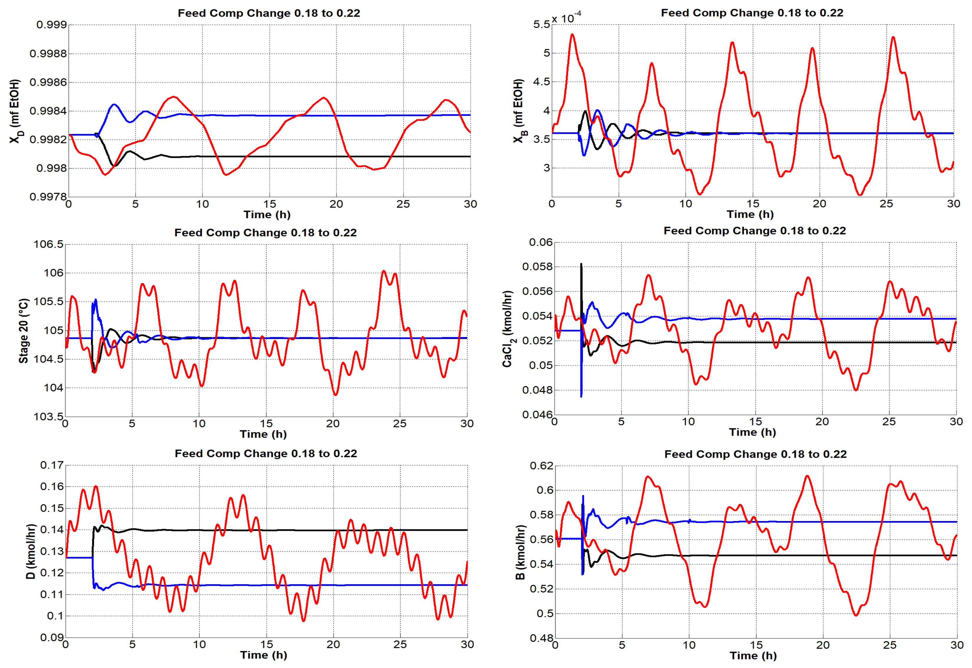
Figure 13 shows the behavior of the process using the $singleend$ structure, called structure L. As can be seen, the maximum composition of the distillate is 99.84% mf and the minimum is 99.80% mf. Moreover, the temperature of tray 20 can be observed, which is the temperature that is controlled to infer and regulate the composition of the distillate; its variation is less than 1 ${}^{°}\mathrm{C}$.

Table 7. The behavior of the process using the structure L. Maximum, minimum, and stabilization values in the event of disturbances in the feed composition.

Step +10%
Variable	$x_D$	$x_B$	$T_{st20}$	D	B	CaCl${}_2$
Unit	mf Ethanol	mf Ethanol	°C	kmol/h	kmol/h	kmol/h
Max	0.998121	3.99 × ${10}^{-4}$	105.024	0.141956	0.588668	0.0582371
Min	0.998014	3.33 × ${10}^{-4}$	104.280	0.138807	0.532195	0.0507858
Stable	0.998083	3.61 × ${10}^{-4}$	104.868	0.139771	0.547100	0.0518722
Step $-10$%
Variable	$x_D$	$x_B$	$T_{st20}$	D	B	CaCl${}_2$
Unit	mf Ethanol	mf Ethanol	°C	kmol/h	kmol/h	kmol/h
Max	0.998446	4.01 × ${10}^{-4}$	105.541	0.115432	0.595486	0.0551621
Min	0.998320	3.22 × ${10}^{-4}$	104.703	0.111892	0.531760	0.0474484
Stable	0.998372	3.60 × ${10}^{-4}$	104.869	0.114279	0.574504	0.0537799
Sinusoidal
Variable	$x_D$	$x_B$	$T_{st20}$	D	B	CaCl${}_2$
Unit	mf Ethanol	mf Ethanol	°C	kmol/h	kmol/h	kmol/h
Max	0.998501	5.33 × ${10}^{-4}$	106.039	0.160277	0.611958	0.0573512
Min	0.997955	2.53 × ${10}^{-4}$	103.873	0.097508	0.498345	0.0479607

summarizes Figure 13 and reports the maximum and minimum values, as well as the value at which it stabilizes in a given time. On the other hand, when the disturbance is oscillatory, the maximum composition reached by the distillate is 99.85% mf with a minimum composition of 99.79% mf, giving rise to a variation of less than 3 ${}^{°}\mathrm{C}$. These data are important since in the next section we will talk about performance and energy saving.

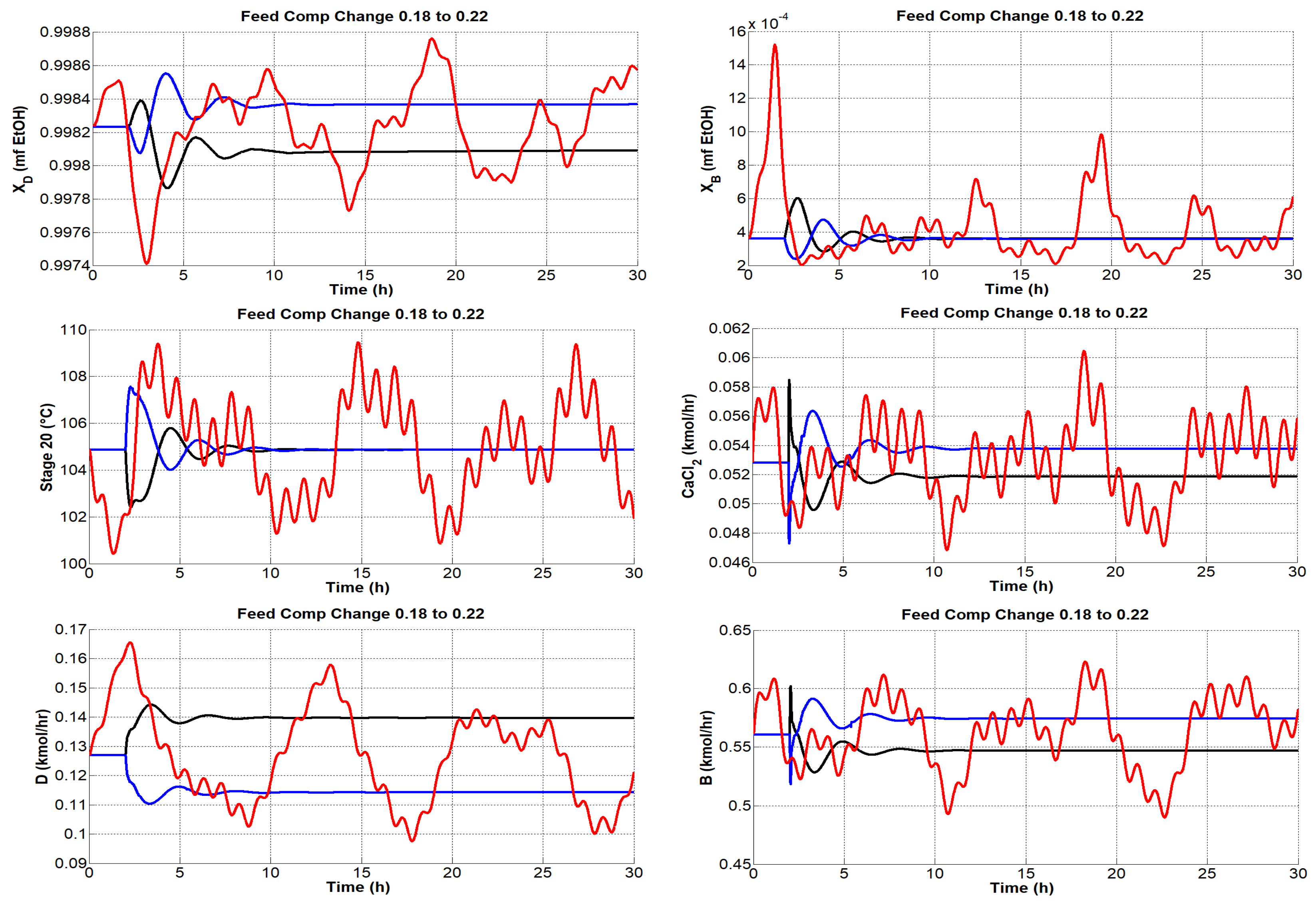
In Figure 14, in the same way, the behavior of the process is reported using the structure of a control point called structure D, and it is observed that the composition of the distillate is greater than that reported in the previous structure, with a maximum composition of 99.85% mf but with a drop that is also greater (99.78% mf), and the variation in temperature is greater than 9 ${}^{°}\mathrm{C}$.

Table 8. The behavior of the process using structure D. Maximum, minimum, and stabilization values in the event of disturbances in the feed composition.

Step +10%
Variable	$x_D$	$x_B$	$T_{st20}$	D	B	CaCl${}_2$
Unit	mf Ethanol	mf Ethanol	°C	kmol/h	kmol/h	kmol/h
Max	0.998391	6.03 × ${10}^{-4}$	105.801	0.144284	0.601945	0.0584786
Min	0.997866	2.83 × ${10}^{-4}$	102.393	0.137889	0.528555	0.0495736
Stable	0.998093	3.61 × ${10}^{-4}$	104.867	0.139769	0.54710	0.0518725
Step $-10$%
Variable	$x_D$	$x_B$	$T_{st20}$	D	B	CaCl${}_2$
Unit	mf Ethanol	mf Ethanol	°C	kmol/h	kmol/h	kmol/h
Max	0.998554	4.74 × ${10}^{-4}$	107.576	0.116237	0.591421	0.0563562
Min	0.998077	2.40 × ${10}^{-4}$	104.014	0.110399	0.518455	0.0473115
Stable	0.998370	3.60 × ${10}^{-4}$	104.869	0.114281	0.574501	0.0537792
Sinusoidal
Variable	$x_D$	$x_B$	$T_{st20}$	D	B	CaCl${}_2$
Unit	mf Ethanol	mf Ethanol	°C	kmol/h	kmol/h	kmol/h
Max	0.998764	1.52 × ${10}^{-4}$	109.457	0.165528	0.622933	0.0604465
Min	0.997413	2.03 × ${10}^{-4}$	100.421	0.0975075	0.490046	0.0468456

summarizes Figure 14 and reports the maximum and minimum values, as well as the value at which it stabilizes in a given time.

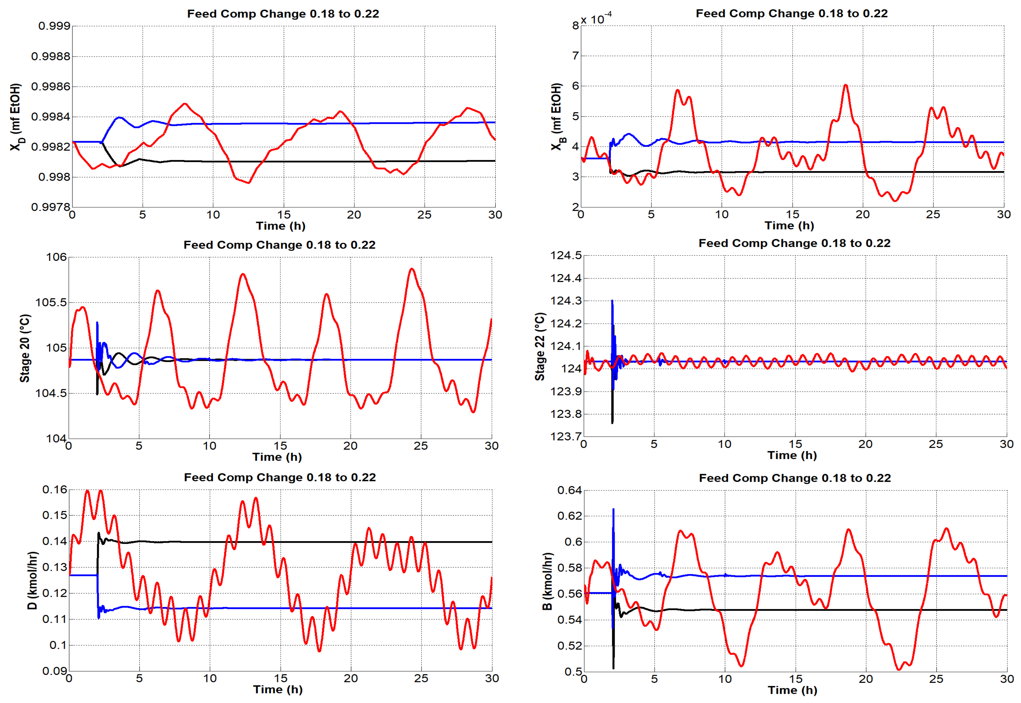
Figure 15 shows the behaviors of the process disturbances in the feed composition in the step and sinusoidal form but now using the two control point structures, called the LV structure. In this figure, you can see the behavior of the composition in the distillate.

Table 9. The behavior of the process using the structure LV. Maximum, minimum, and stabilization values in the event of disturbances in the feed composition.

Step +10%
Variable	$x_D$	$x_B$	$T_{st20}$	$T_{st22}$	D	B	CaCl${}_2$
Unit	mf Ethanol	mf Ethanol	°C	°C	kmol/h	kmol/h	kmol/h
Max	0.998120	3.21 × ${10}^{-4}$	105.009	124.192	0.143392	0.586551	0.0582454
Min	0.998072	3.04 × ${10}^{-4}$	104.488	123.760	0.139364	0.502541	0.0516178
Stable	0.998108	3.16 × ${10}^{-4}$	104.868	124.033	0.139793	0.547733	0.0525258
Step $-10$%
Variable	$x_D$	$x_B$	$T_{st20}$	$T_{st22}$	D	B	CaCl${}_2$
Unit	mf Ethanol	mf Ethanol	°C	°C	kmol/h	kmol/h	kmol/h
Max	0.998397	4.02 × ${10}^{-4}$	105.281	124.302	0.114838	0.625463	0.0545912
Min	0.998331	3.54 × ${10}^{-4}$	104.724	123.911	0.110321	0.533903	0.0474512
Stable	0.998363	4.15 × ${10}^{-4}$	104.869	124.032	0.114250	0.573868	0.0531231
Sinusoidal
Variable	$x_D$	$x_B$	$T_{st20}$	$T_{st22}$	D	B	CaCl${}_2$
Unit	mf Ethanol	mf Ethanol	°C	°C	kmol/h	kmol/h	kmol/h
Max	0.998489	6.05 × ${10}^{-4}$	105.873	124.080	0.159720	0.610631	0.0562294
Min	0.997961	2.20 × ${10}^{-4}$	104.288	123.976	0.0975056	0.501391	0.0492466

reports the maximum and minimum values that this behavior has; it should be noted that the maximum composition in the distillate is $99.84$% mf and with a minimum composition of $99.80$% mf. These compositions are very similar to the one reported in structure L but with a difference in the temperature variation in tray 20, which is reported with a variation of $0.5$ ${}^{°}\mathrm{C}$; in addition, the temperature of tray 22 is also regulated, with a variation of $0.4$ ${}^{°}\mathrm{C}$ between its maximum and minimum temperature value. On the other hand, the temperature variation in trays 20 and 22 due to sinusoidal disturbances are less than $0.8$ ${}^{°}\mathrm{C}$ and $0.1$ ${}^{°}\mathrm{C}$, respectively.

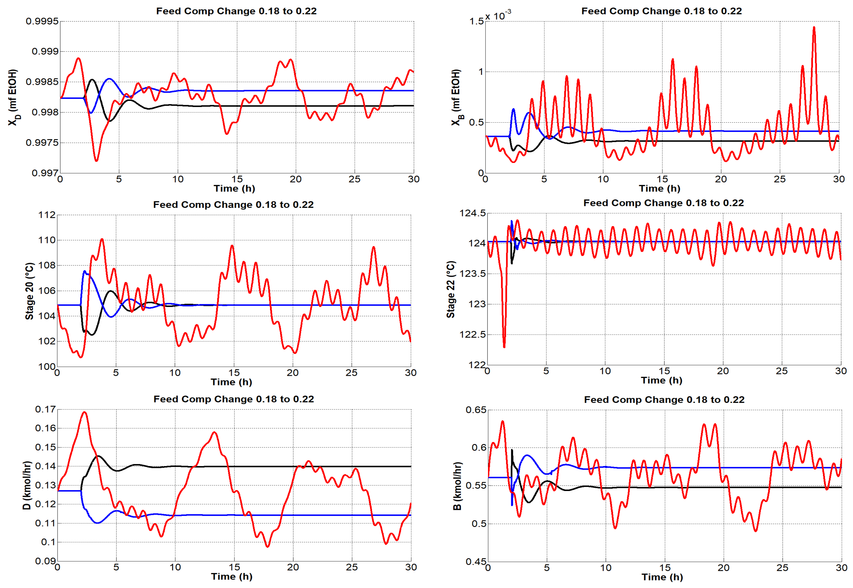
Figure 16 and

Table 10. The behavior of the process using the structure DV. Maximum, minimum, and stabilization values in the event of disturbances in the feed composition.

Step +10%
Variable	$x_D$	$x_B$	$T_{st20}$	$T_{st22}$	D	B	CaCl${}_2$
Unit	mf Ethanol	mf Ethanol	°C	°C	kmol/h	kmol/h	kmol/h
Max	0.998542	3.69 × ${10}^{-4}$	105.98	124.094	0.145368	0.597597	0.0609018
Min	0.997857	2.13 × ${10}^{-4}$	102.511	123.669	0.137537	0.527991	0.0512330
Stable	0.998107	3.16 × ${10}^{-4}$	104.868	124.033	0.139792	0.547733	0.0525263
Step $-10$%
Variable	$x_D$	$x_B$	$T_{st20}$	$T_{st22}$	D	B	CaCl${}_2$
Unit	mf Ethanol	mf Ethanol	°C	°C	kmol/h	kmol/h	kmol/h
Max	0.998554	6.33 × ${10}^{-4}$	107.564	124.374	0.116504	0.590163	0.0546879
Min	0.997988	3.36 × ${10}^{-4}$	103.930	123.899	0.110041	0.524405	0.0465062
Stable	0.998356	4.15 × ${10}^{-4}$	104.868	124.032	0.114250	0.573868	0.053119
Sinusoidal
Variable	$x_D$	$x_B$	$T_{st20}$	$T_{st22}$	D	B	CaCl${}_2$
Unit	mf Ethanol	mf Ethanol	°C	°C	kmol/h	kmol/h	kmol/h
Max	0.998891	1.44 × ${10}^{-4}$	110.100	124.381	0.168601	0.635268	0.0780738
Min	0.997195	1.06 × ${10}^{-4}$	100.729	122.289	0.0974516	0.490038	0.0440028

report the behavior of the process and its maximum and minimum values using the structures of two control points, called structure DV. In this figure, you can see the behavior of the composition in the distillate, the behavior of the temperatures in tray 20 and tray 22, as well as their flows, both in the distillate and in the residue. In Table 10, a maximum value is reported in the distillate of $99.85$% mf and with a minimum value of $99.78$% mf. In addition, with maximum temperatures of $107.52$ ${}^{°}\mathrm{C}$ and $124.37$ ${}^{°}\mathrm{C}$ in tray 20 and tray 22, respectively.

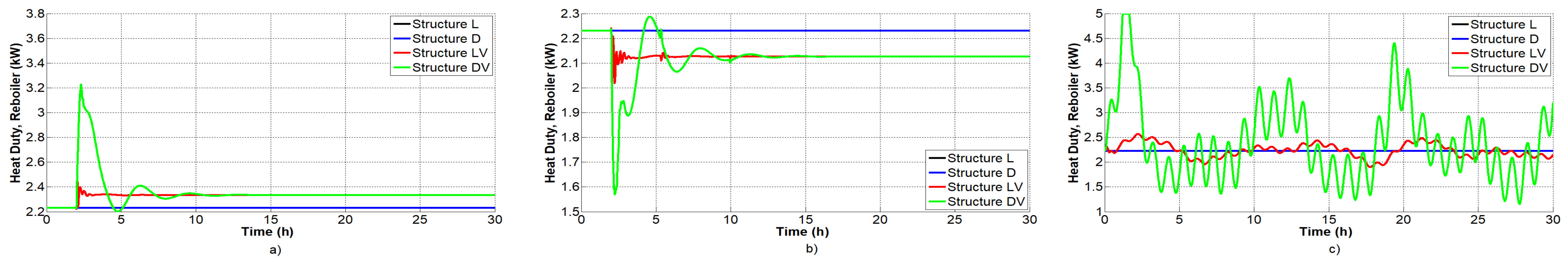
Figure 17 reports the behavior of the reboiler using the four different structures previously described. These figures compare the behavior of each of the structures. To make a better comparison, the maximum and minimum values of the energy consumed are reported in

Table 11. Energy consumption of the reboiler when using control structures. Reboiler energy consumption user the control structure. Maximum, minimum, and stabilization values in the event of disturbances in the feed composition.

Step +10%
Structure	L	D	LV	DV
Unit	kW	kW	kW	kW
Max	2.23188	2.23188	2.46885	3.22535
Min	2.23188	2.23188	2.22401	2.20217
Stable	2.23188	2.23188	2.33474	2.33475
Step $-10$%
Structure	L	D	LV	DV
Unit	kW	kW	kW	kW
Max	2.23188	2.23188	2.23961	2.28785
Min	2.23188	2.23188	2.00574	1.57068
Stable	2.23188	2.23188	2.12697	2.12697
Sinusoidal
Structure	L	D	LV	DV
Unit	kW	kW	kW	kW
Max	2.23188	2.23188	2.57011	5
Min	2.23188	2.23188	1.90333	1.15684

. Based on this table, it can be summarized that for structures L and D, there is no excess energy consumption, because the temperature of the reboiler is not controlled, it remains constant; however, for structure DV, an increase in energy consumption is reported. The energy of up to more than 200% makes this structure the worst used to control this type of process.

6.2. Analysis of Error Results

The results of the evaluation of the performance of the control structures based on the integral error criteria are summarized in

Table 12. Summary of the error indices of the control structures before the disturbances in the composition of the main feed.

Structure L
Perturbation	Bias ×${10}^{-3}$	ISE	IAE	ITAE${}_{set}$	ITAE${}_{nss}$	Average Heat Duty${}_{reboiler}$ (kW)
Step (+10)	0.152	6.39 × ${10}^{-5}$	0.418	6.782	0.117	2.2318
Step (−10)	−0.138	5.11 × ${10}^{-5}$	0.373	6.039	0.237	2.2318
Sinusoidal		7.88 × ${10}^{-5}$	0.429	6.543		2.2318
Structure D
Perturbation	Bias ×${10}^{-3}$	ISE	IAE	ITAE${}_{set}$	ITAE${}_{nss}$	Average Heat Duty${}_{reboiler}$ (kW)
Step (+10)	0.142	$6.96$ × ${10}^{-5}$	0.424	6.642	0.493	2.2318
Step (−10)	−0.135	$5.57$ × ${10}^{-5}$	0.380	6.010	0.334	2.2318
Sinusoidal		$1.55$ × ${10}^{-4}$	0.572	8.939		2.2318
Structure LV
Perturbation	Bias ×${10}^{-3}$	ISE	IAE	ITAE${}_{set}$	ITAE${}_{nss}$	Average Heat Duty${}_{reboiler}$ (kW)
Step (+10)	0.127	$4.66$$\times$${10}^{-5}$	0.359	5.789	0.158	2.3284
Step (−10)	−0.128	$4.13$$\times$${10}^{-5}$	0.337	5.503	0.279	2.1335
Sinusoidal		$5.83$$\times$${10}^{-5}$	0.369	5.623		2.2263
Structure DV
Perturbation	Bias ×${10}^{-3}$	ISE	IAE	ITAE${}_{set}$	ITAE${}_{nss}$	Average Heat Duty${}_{reboiler}$ (kW)
Step (+10)	0.128	$6.09$$\times$${10}^{-5}$	0.387	5.884	0.432	2.3568
Step (−10)	−0.121	$4.94$$\times$${10}^{-5}$	0.352	5.446	0.3608	2.1235
Sinusoidal		$2.00$$\times$${10}^{-4}$	0.645	9.943		2.3411

,

Table 13. Summary of the error indices of the control structures before the disturbances in the feed flux main rate.

Structure L
Perturbation	Bias $\times {10}^{-3}$	ISE	IAE	ITAE${}_{set}$	ITAE${}_{nss}$	Average Heat Duty${}_{reboiler}$ (kW)
Step (+10)	−0.005	$4.61$$\times$${10}^{-6}$	0.052	0.338	0.444	2.2318
Step (−10)	−0.011	$3.06$$\times$${10}^{-6}$	0.053	0.446	0.170	2.2318
Sinusoidal		$3.39$$\times$${10}^{-6}$	0.082	1.149		2.2318
Structure D
Perturbation	Bias ×${10}^{-3}$	ISE	IAE	ITAE${}_{set}$	ITAE${}_{nss}$	Average Heat Duty${}_{reboiler}$ (kW)
Step (+10)	0.002	$1.57$$\times$${10}^{-5}$	0.083	0.431	0.361	2.2318
Step (−10)	−0.013	$1.18$$\times$${10}^{-5}$	0.088	0.731	0.345	2.2318
Sinusoidal		$5.67$$\times$${10}^{-5}$	0.319	4.767		2.2318
Structure LV
Perturbation	Bias ×${10}^{-3}$	ISE	IAE	ITAE${}_{set}$	ITAE${}_{nss}$	Average Heat Duty${}_{reboiler}$ (kW)
Step (+10)	−0.019	$1.80$$\times$${10}^{-6}$	0.059	0.831	0.131	2.3547
Step(-10)	0.007	$1.81$$\times$${10}^{-6}$	0.049	0.543	0.255	2.1170
Sinusoidal		$2.50$$\times$${10}^{-6}$	0.069	1.003		2.2427
Structure DV
Perturbation	Bias ×${10}^{-3}$	ISE	IAE	ITAE${}_{set}$	ITAE${}_{nss}$	Average Heat Duty${}_{reboiler}$ (kW)
Step (+10)	−0.016	$2.72$$\times$${10}^{-5}$	0.136	1.111	0.491	2.4041
Step (−10)	0.021	$1.72$$\times$${10}^{-5}$	0.109	0.996	0.456	2.0985
Sinusoidal		$9.62$$\times$${10}^{-5}$	0.416	6.170		2.3017

and

Table 14. Summary of the error rates of the control structures in the face of simultaneous disturbances in the composition and feed flow.

Structure L
Perturbation	ISE	IAE	ITAE${}_{set}$	Average Heat Duty${}_{reboiler}$ (kW)
Sinusoidal	$8.212$$\times$${10}^{-5}$	0.439	6.665	2.2318
Structure D
Perturbation	ISE	IAE	ITAE${}_{set}$	Average Heat Duty${}_{reboiler}$ (kW)
Sinusoidal	$2.044$$\times$${10}^{-4}$	0.620	9.030	2.2318
Structure LV
Perturbation	ISE	IAE	ITAE${}_{set}$	Average Heat Duty${}_{reboiler}$ (kW)
Sinusoidal	$6.335$$\times$${10}^{-5}$	0.382	5.943	2.2367
Structure DV
Perturbation	ISE	IAE	ITAE${}_{set}$	Average Heat Duty${}_{reboiler}$ (kW)
Sinusoidal	$2.965$$\times$${10}^{-4}$	0.728	10.284	2.4104

.

Structure D generates the highest values of ISE, IAE, and ITAE, with the exception of bias, since structure L is the one that results in the highest value, meaning that structure L has a greater deviation with respect to the reference; however, structure D shows poor performance when compared to the other errors of structure L and the other control structures. On the other hand, the step disturbances in the input variables generate higher values of ITAE${}_{ref}$, which indicate that the errors in the stable state affect the plant more than the action of the controller; moreover, ITAE${}_{nee}$ indicates that the response of the controller is oscillating, resulting in the D and DV structures having higher overshoots. The DV and LV structures, dispute the bias, ISE, IAE, and ITAE${}_{ref}$ errors between intermediate to low values. However, the errors of the ITA${}_{nee}$ of the DV structure are close to those of the D structure, which means that the action of the controller is similar. However, the LV and DV control structures have comparable trade-offs, no matter what type of disturbance is introduced.

For all the evaluated structures, the saline extractive distillation column will behave as non-linear, in which it will produce ‘bias’ compositions in the distillate, depending on whether the disturbance corresponds to an increase or a decrease in the input variables. In addition, the positive and negative step perturbation gives much smaller ITAE${}_{nee}$ than the ITAE${}_{ref}$, which means that the steady-state error is oscillatory.

Therefore, these structures detect such controller behaviors. The results of the simulations with positive changes in the composition of the main feed yield an ISE and an ITAE${}_{ref}$, as well as that of the oscillations.

Monitoring of the heat of the closed-loop reboiler reveals that under changes in composition and feed flow, the $singleend$ control structures maintain an average power equal to the nominal value of 2.23 kW, due to the reboiler heat. However, for the $dualend$ structures, the energy consumption is proportional to the changes in the composition of the feed, giving rise to large deviations in energy consumption (but they are very close to the nominal condition).

As mentioned above, different types of simulations were carried out, but the graphs only reported disturbances in the composition of the feed. Table 13 reports the performance of the control against disturbances in the feed flow of ± 10% (from 0.5715 to 0.6985). These perturbations had the same shapes as the perturbations described in the disturbances Section 4.1. The performances of these structures were evaluated using error and energy consumption criteria.

In summary, the steady-state deviations caused by disturbances in the feed flow are small compared to those caused by disturbances in the composition of the feed. The L structures all lead to errors smaller than those of the DV structure but similar to that of the LV structure due to overshoot. On the contrary, the L and D structures have lower power consumption in the reboiler compared to the LV and DV structures, because there is no interaction of a controller in the reboiler.

Finally, the control structures were simulated in the face of simultaneous sinusoidal variations in the flow and the composition of the main feed. The results of these simulations are reported in Table 14 and Figure 17; it can be seen that the control performance fell, causing a simple effect on the composition of the distillate; however, the standards of purity are still maintained. The L and LV structures improve the transient response of the composition in the distillate since they have the lowest values of the ISE and IAE indices. In addition, the heat of the reboiler is constant.

The measurement of the energy consumption of the reboiler complements the classification of the control structures, showing that the control structure’s $singleend$ saves more energy than any structure’s $dualend$ before any type of disturbance.

7. Conclusions

In this investigation, four different classical control structures were applied and evaluated, which were tuned using the Ziegler-Nichols oscillation method. The objective of using this type of structure is to provide a reference in the control of the process using a saline distillation column, regardless of the salt used, since there are very few reports on the control of this type of column due to: its high non-linearity, a second feed, and the introduction of a solid salt; moreover, it was given a realistic effect by considering the system dynamics, size, efficiency, and common disturbances.

On the other hand, from the point of view of the international purity standard for bioethanol, it can be concluded that a good result was obtained in the application of the control structures by manipulating the temperatures, since no procedure was found in the literature for the selection of trays for the inferential control of composition for this type of extractive distillation column, so it was a good exercise to test the procedure described by Luyben for binary distillation columns; in addition, the results of the simulation of the salt extractive distillation columns are reported using the interaction parameters obtained through the Aspen Plus DRS^®, indicating a difference of less than 1% in error in the composition and temperature with respect to the experimental data reported by Nishi.

In general, for this case study in which four control structures (L, D, LV, and LD) were compared, the analysis of the results of the applied error criteria shows that for this process the structures of a control point are the best options, since the flow or heat in the reboiler is not manipulated; therefore, the energy is kept constant by step disturbances in the composition and the inlet flow of the main feed, causing a lower consumption of energy during the entire operation time of the column. In particular, for the reasons mentioned above, the L structure is the one with the best performance; this conclusion is confirmed by the reported results on error rates and power consumption.

This work can be used as a case study on the dehydration of ethanol as well as a simulation of the control of structures, since it meets the necessary characteristics to put it into practice.