A Sustainable Supply Chain Integrated with Autonomated Inspection, Flexible Eco-Production, and Smart Transportation

Abstract

The present study focuses on supply chain management to improve its sustainability from economic, environmental, and social perspectives. First, improving production process reliability and cost reduction are two main factors for enhancing economic sustainability. Hence, we introduced autonomated inspection and invested in ordering and setup costs. Second, reducing the carbon footprint in supply chains is the main pillar of their environmental stewardship, which is addressed by an eco-friendly and flexible production system in this study. Finally, an advanced single-setup-multi-delivery (SSMD) strategy is utilized to improve social aspects associated with human labor increase. For practicality, demand is considered as the selling price and is quality dependent. The sustainability enhancement is transformed as a term of profit; therefore, our model maximizes the total profit of the supply chain by optimizing a manufacturer’s and retailer’s decision variables. Numerical examples show that autonomation technology increases the system’s reliability by $64\%$, where eco-production reduces carbon emission by up to $16\%$, and the total profit increases by up to $25\%$. Moreover, the application of advanced SSMD reduces the transportation cost by up to $34\%$.

1. Introduction

Nowadays, sustainable supply chain management (SSCM), which considers the roles of all involved parties, is attracting considerable research focus and interest (Garai and Sarkar [1]). A sustainable supply chain (SC) is one in which the economic, environmental, and social benefits of all involved players are effectively considered (Seok et al. [2]). Environmental sustainability includes factors such as waste management, energy consumption, risk, and recoverability. Social sustainability adopts the concept of employee satisfaction, quality of life, reputation, and visibility. Economic sustainability increases profits or decreases costs. By using some advanced technologies, the sustainability of the supply chain can be enhanced (Sardar et al. [3], Dumitrascu et al. [4]). In this study, we developed a supply chain model and investigated its sustainability from the economic, environmental, and social perspectives. This is performed by applying an intelligent autonomated inspection and investments in the setup, reducing ordering costs, which enhances the economic sustainability of the chain by reducing the supply chain’s total cost. In addition, eco-production was inspected by employing green costs to assess environmental sustainability. Social aspects were addressed by using an advanced single-setup-multi-delivery (SSMD) to recruit labor forces. To the best of our knowledge, such an approach has not been previously reported in the literature. A more detailed explanation is provided as follows.

To improve the economic sustainability of the supply chain, two approaches were adopted in this study. First, we make use of an advanced autonomated inspection to increases production’s reliability. This is manifested through the reduction of defective components and products, which eventually leads to growing the business’s profit (Dey et al. [5]). Second, we consider ways to reduce ordering costs. In fact, the ordering policy plays a vital role in the sustainability of supply chains (Sarkar and Chung [6]). Ordering cost has been considered as fixed in most previously reported supply chain models. Nevertheless, a retailer or customer could cancel their orders at any time due to quality defects, lead time, or other issues. Certain costs should be passed to retailers if orders are cancelled, which can save some investment costs. Therefore, treating such ordering costs as a model variable is more reasonable. Consider the following example, retailers use the Internet or mobile phones to make or cancel orders. The mobile or Internet service provider could have different tariff plans. Thus, if retailers effectively invest money for their mobile/Internet plan, they can reduce their per-unit ordering cost. Similarly, if a company invests money in the setup process of its production system, the total setup cost could thus be reduced (Sarkar & Chung [6], Dey et al. [7], Sarkar et al. [8]).

To improve the environmental sustainability of the supply chain, an eco-production system is introduced in this model. In fact, the high consumption of non-biodegradable and non-environmentally friendly products is the major source of continuous environmental pollution. Most reported research focuses on environmentally friendly products in an attempt to reduce carbon emissions (Sana [9], Mishra et al. [10], Liu et al. [11]). However, reported approaches are mainly limited to the design of eco-friendly products or process investment to reduce carbon emissions (Sana [9], Sepehri et al. [12]). Nonetheless, the direct consideration of a greening unit production cost has not been investigated thus far. Therefore, we developed a novel eco-production system model considering the approach of greening costs in this study.

Lastly, we improve social sustainability by a smart transportation policy. In general, a manufacturer bears transportation costs for transferring products to retailers’ warehouses. Conversely, for the return of a defective product, the retailer bears transportation costs. In most existing studies such transportation costs are assumed to be fixed, or sometimes variable depending on the quantity (Sarkar et al. [13], Sarkar et al. [14]). Nevertheless, in general, the capacity of a container and distance between the manufacturer’s and retailer’s warehouses are transportation costs. Therefore, in this study, an advanced single-setup-multi-delivery (SSMD) policy is utilized, in which transportation costs vary depending on the distance, capacity of the container, and quantity. This contributes to enhancing the social sustainability of a supply chain increasing human labor. At first glance, increasing the number of workers might seem to increase labor costs, which reduces profits. However, adopting the SSMD transportation policy, lead time will be reduced, which in turn enhances the profit of the entire supply chain. This installs an important link between social sustainability and the implementation of the SSMD transportation policy. Figure 1 represents the enhancement means of the three basic pillars of sustainability as addressed in this study. The main contributions of this study could be classified as follows:

(i)

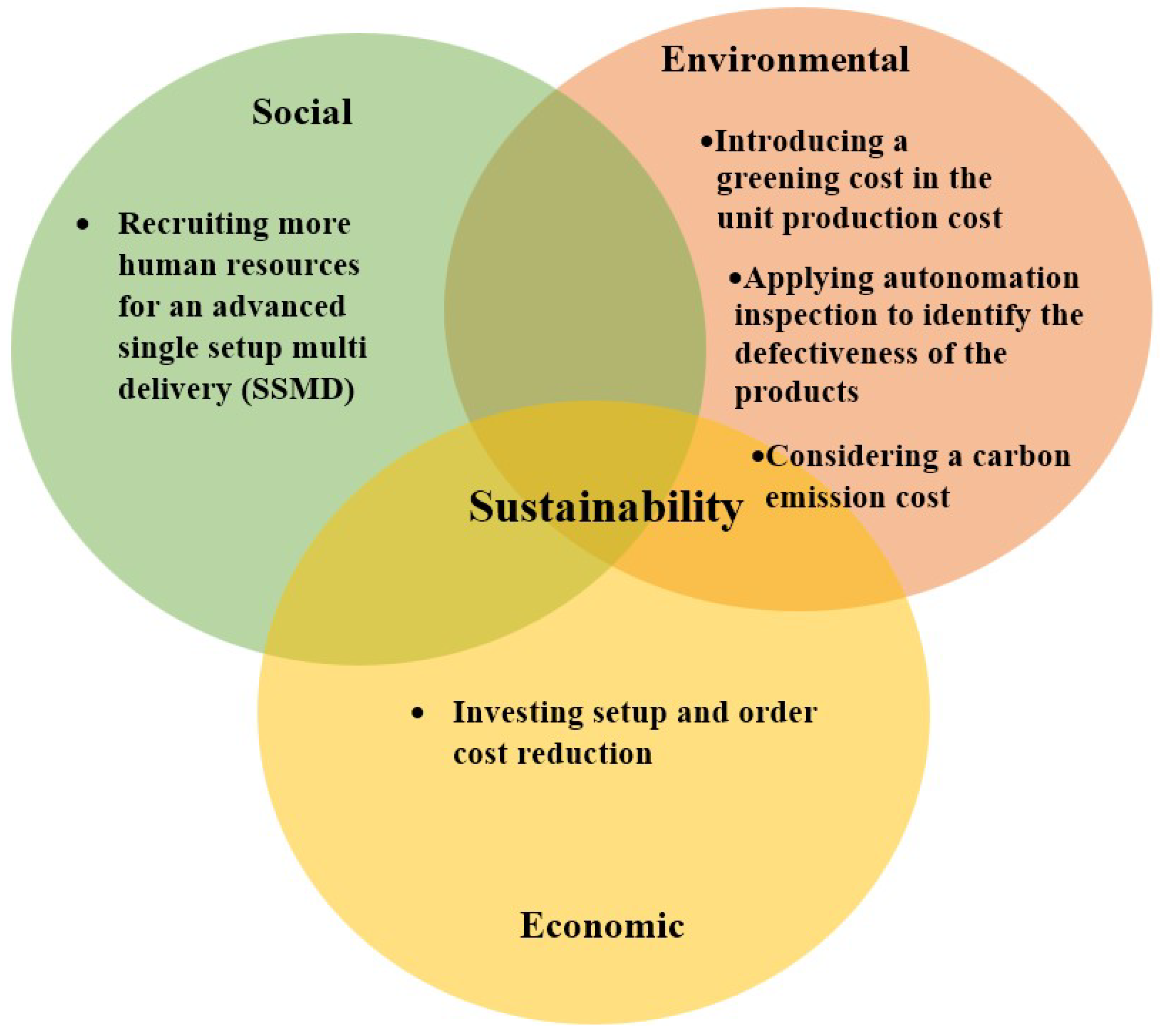
Several supply chain models were designed based on the concept of sustainability [9,15,16]. However, a sustainable supply chain model, in which smart autonomated inspection is considered to enhance reliability, has not been reported so far. Thus, an effort is made in the present study to incorporate smart autonomation technology which enhances the system’s reliability and economic sustainability.

(ii)

Many supply chain models dealt with a fixed ordering cost, and fixed setup cost [17,18,19]. However, these approaches lack practicability. Thus, in this study, we consider these costs as model variables, especially when they can be reduced by some investment. This constitutes a new approach to enhance the economic sustainability of a supply chain.

(iii)

Most of the studies set the production cost based only on the material cost, development cost, and die/tools cost [20,21]. To make an environment friendly product, we introduce environment-related costs in unit production cost directly.

(iv)

The SSMD strategy concept has been utilized in some previously reported supply chain models [18,22,23,24]. Nonetheless, the quantity, container, and distance-dependent advanced transportation strategy remained largely unexplored. Here, we employ such an advanced SSMD policy to make the system more socially sustainable.

(v)

For more practicality, selling price, product-quality-dependent demand, and a variable production rate are considered.

As a result, we optimize the quantity and safety factor, lead time of the retailer, production rate, investment for setup cost reduction, and probability for transferring under-control to out-of-control state of the manufacturer, while enhancing the sustainability as described above.

More detailed background and motivation of the current study are described in Section 2. Compared to the existing literature, the uniqueness of this research is summarized in

Table 1. Existing supply chain study with different objectives.

Researchers	Process Reliability	Demand Depend on	Production Rate	Investment for Setup & Order Cost Reduction	Transportation Policy
Dey et al. [5]	NA	SPQ	Var.	NA	NA
Dey et al. [7]	Inc.	SP	Con.	SC	SSMD
Hong & Guo [25]	NA	Con.	Con.	NA	NA
Huang et al. [26]	NA	Con.	Con.	SC	NA
Khouja & Mehrez [27]	NA	Con.	Var.	NA	NA
Kim et al. [22]	NA	Con.	Var.	NA	SSMD
Majumder et al. [28]	Inc.	Con.	Var.	SC	SSMD
Pal et al. [17]	NA	SP	Con.	NA	NA
Sarkar et al. [8]	Inc.	Con.	Con.	SC	SSSD
Sarkar and Chung [6]	Inc.	Con.	Var.	SC	SSMD
Yu & Han [29]	NA	Con.	Con.	NA	NA
This study	AI	SPQ	Var.	SOC	Smart
					SSMD

NA-not applicable; SPQ-selling price and quality; Var.-variable; Inc.-increment of the production process reliability; SP-selling price; Con.-constant; SC-setup cost; SSMD-single setup multi delivery; SSSD-single setup single delivery; AI-autonomation policy is utilised to increase the reliability of the production process; SOC-setup and ordering cost.

. The mathematical model and its extension are described in Section 3. The solution methodology along with a lemma and advanced algorithm is presented in Section 4. Some numerical examples with exceptional cases and a comparison with existing literature are presented in Section 5, and the effect of critical parameters on the total profit is presented in Section 6. The implementation of the study in form of industrial benefits are discussed in Section 7. Finally, discussions regarding this model, its applications, limitations, and future extensions are presented in Section 8.

2. Background and Motivation

In Table 1, our present study is compared to previous works from the literature. Differences are emphasized and details are discussed in the following sections.

2.1. Autonomated Inspection

Several factors could have a negative impact on a supply chain’s profit and reliability such as defective products, which may result from various issues related to machine failure or labor inconsistency (Sarkar et al. [30]). Among several ways proposed to enhance the process quality, the investment to increase the quality of the production process has been the most applied approach (Sarkar et al. [8], Majumder et al. [28], Sarkar and Chung [6]). Nonetheless, smart autonomation is one of the ways used to identify defective products to increase the system’s reliability and product quality (Dey et al. [5]). Autonomation can be used as a machine-based inspection, capable of faster and more systematic defectiveness detection compared to human-based inspections. We thus consider in this study the continuous investment for autonomation inspection to ultimately increase the economic sustainability of a system by reducing unnecessary waste by increasing process reliability. In particular, the autonomation policy is primarily employed where demand varies with the selling price and quality of the product under a variable production rate in the current model (Table 1). These conditions enhance the practicability of make our proposed model.

2.2. Order and Setup Cost Reduction

To run a business, the retailer has to place some orders for products. Most previous researchers considered a fixed retailer’s ordering cost [31,32] and optimized the lot size to minimize it. In this study, we consider the ordering cost as a variable in our model and develop ways to reduce it by some investments, for an improved practicality.

On the one hand, an order can be placed in different ways, such as online, offline, or by making a phone call. Tariff charges for Internet or phone calls can vary among service providers. Moreover, customers can cancel or modify their order with uncertain corresponding charges. Thus, assuming the ordering cost as a fixed quantity reduces the flexibility and practicality of a model. The investment in phone and Internet bill plans could partially reduce such retailing ordering and cancellation costs.

On the other hand, a manufacturer always tends to reduce setup costs. In fact, the approach of setup cost reduction through some investment in the production system was first introduced by Porteus [33]. He proved that continuous investment is an effective way to reduce setup cost. This is translated in two investment phases. Investments during the startup phase of the manufacturing process by incorporating good quality machines and during the manufacturing phase by ensuring a good machines and equipment maintenance contribute largely to reducing the setup cost (Sarkar et al. [8]). Sarkar et al. [8] optimized the setup cost, order quantity, reorder point, and manufacturing process probability for shipment of under-control to out-of-control situations. Majumder et al. [28] and Dey et al. [34] developed supply chain models for multiple retailers and single manufacturer, where ordering cost was reduced by discrete investment. Sarkar and Chung [6] developed a flexible supply chain model, where a discrete investment was utilized to reduce the setup cost. However, a two-echelon supply chain model for a single item with investments for both order and setup costs reduction has not been reported yet. We first propose a sustainable supply chain model, where both setup and order costs can be reduced through some discrete investment in which ordering cost is calculated by summing the original cost for order and order cancellation costs.

2.3. Eco-Production

Environmental benefits are the key components of a sustainable supply chain model. The life cycle of a deteriorating environment friendly product was proposed by Wee et al. [35] who discussed the optimal replenishment policy, cost analysis, and effectiveness of the product’s selling price. The impact of technologies on the market structure of environment friendly products was calculated by Su et al. [36]. The authors proposed an optimized model for the price and quality of products to maximize the supply chain profit. Investments in related technologies were proposed to increase the green quality of products, which has been studied for different market scenarios. A green product manufacturing system, incorporating the concept of carbon regulation to optimize carbon emission, was presented by Halat and Hafezalkotob [37]. The authors considered in their study a multi-stage green supply chain model. To reduce carbon emissions, different carbon regulation policies were discussed in their model for an eco-friendly product. Coordination and non-coordination game strategy was utilized by Halat and Hafezalkotob [37] to obtain the best result along with eight bi-level mathematical programming models. Although environmental and economic aspects are two basic pillars of supply chain sustainability, trade-offs and compromises were required for any production and inventory model to maintain the overall sustainability of the chain (Darvish et al. [38]). Darvish et al. [38] discussed and compared the effect of carbon emission and eco-production on the total system cost. To contribute into the global warming control, eco-friendly production was very much effective (Ahmadini et al. [39]). The authors developed a multi-objective inventory model for manufacturing green products, which is a customer’s attractive approach. On the basis of the production of green or eco-friendly products, a systematic review for the green supply chain model was proposed by Becerra et al. [40]. In their review, the authors considered a total of 91 papers from the existing literature and made comparisons on the basis of technology invention, solution methodology, and optimization techniques. In some cases, the pollution taxation was dependent on the choice of environment friendly products (Yu and Han [29]). Yu and Han [29] proposed a game structure and pollution taxation policy for a supply chain model. Hong and Guo [25] focused on the inventory and procurement strategies, and they considered an additional cost for an environment friendly product. On the other hand, a closed-loop supply chain under remanufacturing was developed by Tang et al. [41]. They developed their model under the Stackelberg game framework including discussions of the green quality of products. Sarkar and Bhuniya [42] developed an imperfect production model, where they considered some investment to produce green product. They also considered variable production rate, where production cost depends on the reliability of the production process. However, they were unaware about the transportation strategy and ordering policies.

Nonetheless, investments towards the improvement of the green quality within the unit production cost have not been addressed thus far.

2.4. Advanced Transportation Strategy

Transportation strategies play a major role in minimizing costs in supply chains. SSMD drives the reduction in setup, ordering, and transportation costs smoothly. In the SSMD policy, the manufacturer starts production soon after receiving the order from the retailer. Production continues up to the end of the production cycle, and products are finally delivered to the retailer in multiple shipments with equal quantities in each shipment, which increases transportation costs for the manufacturer. Hence, an appropriate contract between the manufacturer and retailer can help reduce these costs. Nonetheless, multiple shipments imply a considerably large number of required labor for loading and unloading goods. It means that the SSMD transportation strategy can enhance social sustainability by boosting workability and employment. The concept of the SSMD policy is adopted along with an advanced strategy in this current study. Under this policy, the transportation company charges a fixed cost for transporting a certain number of fixed quantities. A variable transportation cost is utilized for the remaining quantity, which is calculated through unit transportation cost, container capacity, and distance between retailer and manufacturer warehouses.

Several studies employing the SSMD policy in supply chains are reported in the literature. A two-echelon supply chain model under the consideration of the lot-splitting concept, was discussed by Kim and Ha [43]. In their model, the authors considered that the retailer’s order was manufactured with one setup and shipped in equal amounts over multiple deliveries. The model highly reduces the total cost owing to the application of a just-in-time (JIT) lot-splitting strategy with the SSMD policy.

Wang and Sarker [44] proposed a supply chain model for assembled products consisting of a mixed-integer non-linear programming (MINP) problem. They dealt with the Kanban operation between two adjacent plants for loading, unloading, and transportation schedules. They considered that the manufacturer transports the product just after getting the order from the retailer and stops their production until the retailer places new orders. This corresponds to the concept of single setup single delivery (SSSD) transportation policy. However, in SSSD, as the lead time increases, retailers are forced to wait until the products are completed and delivered to them (Sarkar et al. [13]). Kim et al. [22] proved that there is a strong relationship between retailer and supplier through the SSMD policy compared to the single setup single delivery (SSSD) policy due to the increase in lead time. In SSSD transportation policy, manufacturers start production every time after receiving the order from the retailer and make the exact same amount of the ordered quantity. Due to SSSD, retailers, as well as customers, have to wait more compared to SSMD, as in SSMD, the manufacturer can deliver instantly after receiving the order from the retailer but in SSSD, after receiving the order, the manufacturer starts the production, and after production delivers the item to the retailer.

In the global supply chain, players belong to different countries and huge transportation costs are required to run the supply chain smoothly. Sarkar et al. [18] formulated a sustainable global supply chain model in which SSMD policy was utilized to minimize the system’s cost by jointly considering variable carbon emission and variable transportation costs. Their model compared the SSMD with SSSD. A smart supply chain model by considering SSMD policy was developed by Bhuniya et al. [45]. They developed their model under the consideration of flexible manufacturing and concerned about the energy consumption. However, they only considered a fixed transportation cost, whereas the capacity of the container and distance between the players play a vital role for transportation. A bi-objective problem for selective pickup and delivery was proposed by Ben-Said et al. [46]. By using the Pareto Local Search algorithm, they solved their model. They only focus on the pickup and delivery problems and neglect the concept of SSMD and sustainable supply chain.

In contrast to the existing literature, a lot size, container capacity, and distance-dependent variable transportation costs are utilized in our present study, along with the SSMD policy, which makes the supply chain more socially sustainable.

3. Model

3.1. Notation

To make this model more reader friendly, the following notations and assumptions are used:

Decision	Variables
Retailer
$f_s$	safety factor of the inventory
l	lead time to receive a order from manufacturer after placing the order (weeks)
$I_o$	investment to reduce ordering cost ($/order)
Manufacturer
r	production rate of manufacturer (units/time)
$R_p$	probability for transferring the production process to out-of-control state from in-control state, (a probability)
$I_{\omega }$	investment to reduce setup cost ($/setup)
Both players
p	selling price of each item ($/unit)
q	product’s quality level (percentage)
v	number of quantities in each shipment(unit)
z	number of shipments in a lot (unit)
Parameters
$I_{{\omega }_0}$	initial setup cost to run manufacturing process ($/setup)
$B_{\omega }$	setup cost with investments $B_{\omega }\left(I_{\omega }\right)=I_{{\omega }_0}{e}^{-r{I}_{\omega }}$, where r is a parameter
$B_{bv}$	number of a load quantity with a fixed cost from manufacturer to retailer (unit)
$C_b$	retailer’s unit purchase cost per unit ($/unit purchased)
$C_d$	die-tool cost per unit ($/unit)
$C_m$	manufacturing cost per unit ($/unit)
$C_o$	order cancelation cost per item for retailer ($/item) ($/unit)
$E_T$	variable carbon emission cost of manufacturer for transportation per container ($/container)
$F_{CEB}$	fixed carbon emission cost of retailer ($/shipment)
$F_{CV}$	fixed carbon emission cost of manufacturer for transportation ($/shipment)
h	inventory holding cost per unit per unit time of retailer ($/unit/time)
$h_v$	inventory holding cost per unit per unit time of manufacturer ($/unit/time)
$l_{BV}$	distance from retailer’s warehouse to manufacturer’s warehouse (kilometer)
$L\left(l\right)$	consumer’s total number during lead time l
M	demand rate of the retailer (units)
$m_i$	i-th component of lead-time with $m_i$ as crashing cost per unit time ($/unit time), $i=1,2,\cdots ,n$
$M\left(l\right)$	total amount purchased by time l
$M_{uw}$	unit wholesale price of the manufacturer ($/unit)
$O_c$	initial OC for retailer ($/unit)
$Q_{\psi }$	lot size (units)
$R_0$	initial reliability to the imperfect production rate(a probability)
$R\left(l\right)$	total crashing cost related to the lead time ($/week)
S	replenishment cost for defective item ($/unit)
$E_v$	carbon emission cost of manufacturer for production ($/unit)
T	cycle time, $T=Q_{\psi }/M=zv/M$ (time unit)
$T_{C_{f}b}$	fixed transportation cost ($/shipment)
$T_{f_{v}b}$	fixed transportation cost for manufacturer ($/shipment)
$T_{V_{vb}}$	variable transportation cost per container
$u_i$	i-th component of lead time with $u_i$ as minimum duration(days), $i=1,2,\cdots ,n$
$v_i$	i-th component of lead time with $v_i$ as normal duration(days), $i=1,2,\cdots ,n$ per unit distance for manufacturer ($/container.unit distance)
$V_b$	variable cot for transportation per container ($/container/unit distance)
$Y_b$	variable cost for carbon emission of consume by container ($/container)
a, b, r, $\omega$	scaling parameter related to investment
$\alpha$	annual fractional cost related to selling price (a scaling parameter)
$\beta$	price elasticity parameter
$\gamma$	annual fractional cost related to quality (a scaling parameter)
Parameters
$\delta$	quality elasticity parameter
$\chi$	scaling parameter related to retailer transportation cost
$\pi$	unit shortage cost per unit ($/unit shortage)
$\tau$	per unit environmental cost ($/unit)
$\xi$	reorder point
$\varphi$	standard normal probability density function
$\mathsf{\Phi }$	standard normal cumulative distribution function
${\zeta }_b$	capacity of the container of retailer (ton)
${\zeta }_v$	capacity of the container of manufacturer (ton)
$T{C}_R$	total cost for the retailer
$T{P}_R$	total profit for the retailer
$T{C}_M$	total cost for the manufacturer
$T{P}_R$	total profit for the manufacturer
$JETC$	joint expected total cost for the entire SC
$JTP$	joint total profit of the entire SC

3.2. Assumptions

The following assumptions are utilized to develop the current study.

1.

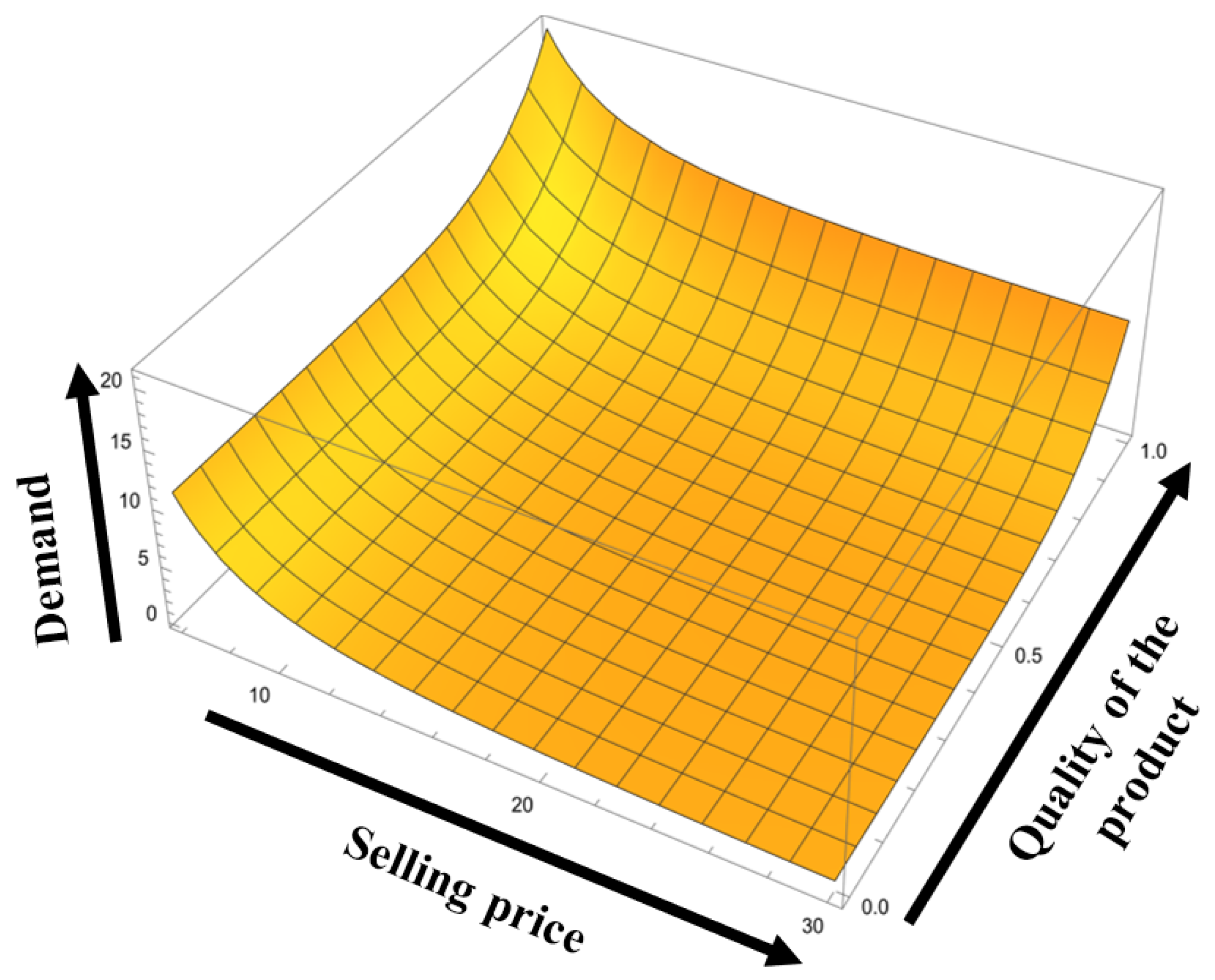
A sustainable supply chain with a single retailer and manufacturer is considered, and a single type of environment friendly product is considered. In reality, customers prefer good quality products at less price. Hence, we assumed that the demand depends on the quality and selling price (Dey et al. [5]) i.e., $M=\alpha p^{-\beta }+\gamma q^{\delta }$ (See Figure 2).

2.

The demand during lead time is unpredictable. Thus, it is considered that the demand during the lead time $\left[L\right(l\left)\right]$ follows a Poisson distribution with a mean $\lambda l$. The $M_i$ are independent and identically normally distributed with mean $\mu$ and standard deviation $\sigma ,$ and, then $\{M\left(l\right)={\sum }_{(i=1)}^{L\left(l\right)}{M}_i,l\ge 0\}$ is a compound Poisson process ([7]). Due to high demand, shortages are fully backordered. To satisfy customers, safety stock is considered in this research, where the reorder point is calculated by summing up the expected lead time demand and the safety stock, i.e., reorder point $=Ml+f_s\sigma \sqrt{l}$.

3.

Every consumer wants their desired product on their doorstep as early as possible. Thus, lead time reduction can improve service quality. This model introduces several crashing costs for mutually independent components to reduce lead time. It is taken that $v_i$ and $u_i$ are the normal and minimum duration, respectively, for the i-th component, such that the per unit crashing cost $m_i$ satisfies the relation $m_1\le m_2\le \cdots \le m_n$. Let the lead time duration be $l_f$ which let the components $1,2,3,\cdots ,n$ crash to minimum duration, and let $l_0={\sum }_{j=1}^n{v}_j$. Then $l_i=l_0-{\sum }_{j=1}^i(v_j-u_j)$ and the crashing cost expression will be $R\left(l\right)$, $R\left(l\right)=m_i(l_{i-1}-l)+{\sum }_{j=1}^{i-1}{m}_j(v_j-u_j)$ for $i=1,2,\cdots ,n$. [47].

4.

A discrete investment, $B_{\omega }\left(S_{r_i}\right)=I_{{\omega }_0}{e}^{-r{I}_{\omega }},$ where $i=0,1,\cdots ,n$ and $S_{r_0}=0,$ is considered to reduce setup cost ([7]). Moreover, ordering cost consists of order cancellation cost, which is reduced by some investments. The continuous investment for autonomation ([5]) is employed to enhance the reliability of the production process.

5.

An environment friendly product is essential these days to keep our environment clean. Thus, the unit production cost of an item is dependent on variable production rate, material cost, and environment-related costs. The cost expression for unit product is $=c_m+\frac{c_d}{r}+\tau r$ (Dey et al. [20]).

6.

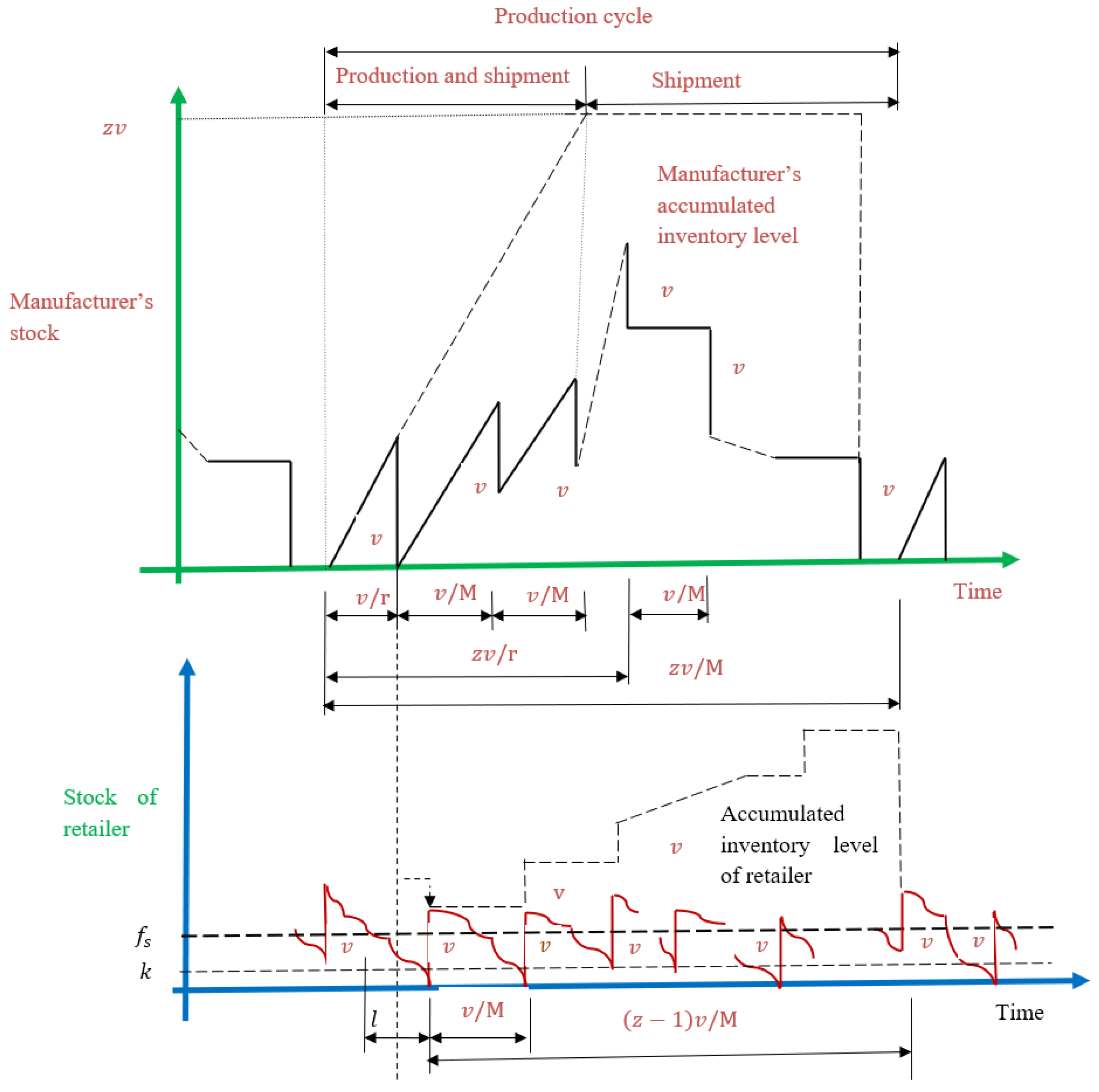
The concept of SSMD policy ([18]) is adopted along with an advanced strategy. The transportation company charges a fixed cost for a certain number of fixed quantities. The rest of the quanity will be delivered by variable transportation costs. It is calculated through unit transportation cost, container capacity, and distance between retailer to manufacturer’s warehouses.

7.

Carbon emission cost is calculated for retailer and manufacturer separately. For retailers, carbon emission is calculated only for transporting the defective product to the manufacturer, whereas for the manufacturer, carbon emission is calculated for transportation and production simultaneously.

3.3. Mathematical Model

In this study, a sustainable SC model is developed for the environment friendly product under different investments. Figure 3 illustrates the inventory positions for the retailer and manufacturer. The profits for each participant are as follows:

3.3.1. Retailer’s Profit

For an advanced SSMD policy, the manufacturer produces the total lot size $Q_{\psi }$ in a single setup and transports to the retailer by z times with shipment volume v. To order, cancel placed orders, or hold the products, different costs are needed. The lead time demand follows a Poisson’s distribution. Thus, according to Dey et al. [7], the lead time demand is $\lambda lu$ and the variance is $Var\left(X\right)=\lambda l(u^2+{\sigma }^2)$. Then the reordered point is given by $\lambda ul+f_s\Sigma \sqrt{\lambda l}$ and shortage per replenishment cycle was $\Sigma \sqrt{\lambda l}\mathsf{\Psi }\left(f_s\right)$, where, ${\Sigma }^2=u^2+{\sigma }^2$, $\mathsf{\Psi }\left(f_s\right)=\varphi \left(f_s\right)-f_s[1-\mathsf{\Phi }\left(f_s\right)]$ and standard normal probability distribution function and cumulative distribution funtion are $\varphi$ and $\mathsf{\Phi }$, respectively.

Now, the average inventory is given by $\left(\frac{v}{2}\right)+f_s\Sigma \sqrt{\lambda l}$

Holding Cost for the Retailer $\left(H{C}_R\right)$

To hold the products, which are ordered by the retailer, some costs are needed. Thus the expected holding cost for the retailer is given as below

$$\begin{array}{c}\hfill h\left[\frac{v}{2}+f_s\Sigma \sqrt{\lambda l}\right]\end{array}$$

(1)

Ordering Cost $\left(O{C}_R\right)$

To run a smooth business, the retailer must order some products from the manufacturer. For this, some costs must be needed, which are known as ordering costs (OCs). Sometimes retailers cancel orders for some reason, which implies some corresponding costs, associated to the ordering cost (OC). Thus the OC, which is the sum of actual OC and cancellation cost for this supply chain, is given by:

$$\begin{array}{c}\hfill \frac{O_c(\alpha p^{-\beta }+\gamma q^{\delta })}{zv}+\frac{C_o(\alpha p^{-\beta }+\gamma q^{\delta })}{zv}\end{array}$$

(2)

Investment to Enhance the Sustainability by Reducing Ordering Cost $\left(IROC\right)$

In this current study, OC is calculated as a sum of original OC and order cancellation cost. The most commonly used technique for placing orders are emails or phone calls. For this, the retailer has to pay some Internet charges or phone bills. It is found that the charges of different service providers vary due to their company policies. These costs could be reduced by considering some investment. Thus, the OC along with investment is given as follows:

$$\begin{array}{c}\hfill \frac{a(O_c+C_o)(\alpha p^{-\beta }+\gamma q^{\delta })}{(a+b{I}_o)zv}+\frac{I_o(\alpha p^{-\beta }+\gamma q^{\delta })}{v}\end{array}$$

(3)

Shortage Cost $\left(S{C}_R\right)$

The demand for a product increases with its high quality, which might drive shortages and variable production rates. The reputation of a company is reduced due to these shortages, which directly disturbs the system profit. Thus, the total shortage cost for this study is calculated as follows:

$$\begin{array}{c}\hfill \frac{\pi (\alpha p^{-\beta }+\gamma q^{\delta })}{v}C\left(\xi \right)\end{array}$$

(4)

Lead Time Crashing Cost $\left(LTCC\right)$

With the advances of communication technologies, customers’ expectations to receive orders instantly has grown considerably. However, everyone is aware of the often required waiting time, known as the lead time. Nonetheless, lead time shortening is another strategy to satisfy customers of any company. Several researchers considered a negligible lead time for SCM; however, it is impossible in reality. Thus, a crashing cost is utilized in this current study to reduce the lead time, which is expressed as follows:

$$\begin{array}{c}\hfill \frac{\alpha p^{-\beta }+\gamma q^{\delta }}{v}R\left(l\right)\end{array}$$

(5)

Smart Transportation Cost for Retailer $\left(ST{C}_R\right)$

Usually, retailers send defective products back to the manufacturers, bearing the corresponding transportation costs. A fixed cost for transporting a minimum quantity $B_{bv}$ is utilized, i.e., the retailer has to pay a fixed cost for transporting up to $B_{bv}$ quantity, whereas any additional $B_{bv}$ quantity, a variable transportation cost will be inferred in the total cost for the retailer. This additional cost is dependent on the distance from the retailer’s warehouse to the manufacturer’s warehouse, the transported quantity, and container capacity.

Thus, the total transportation cost for a retailer is given as follows:

$$\begin{array}{c}\hfill T_{C_{fb}}+V_b\chi \frac{((\alpha p^{-\beta }+\gamma q^{\delta })-B_{bv})}{{\zeta }_b}{l}_{BV}\end{array}$$

(6)

Carbon Emission Cost for Retailer $\left(CE{C}_R\right)$

As a result of transporting defective products, additional carbon emission costs should be paid by the retailer at a fixed and variable carbon emission cost. Thus, the total carbon emission cost for the entire production cycle is obtained as follows:

$$\begin{array}{c}\hfill F_{CEB}+Y_b\chi \frac{(\alpha p^{-\beta }+\gamma q^{\delta })}{{\zeta }_b}\end{array}$$

(7)

Therefore, the total cost for the retailer is

$$\begin{array}{ccc}\hfill T{C}_R(z,v,p,q,I_o,l,f_s)& =& O{C}_R+IROC+H{C}_R+S{C}_R+LTCC+ST{C}_R+CE{C}_R\hfill \\ & =& \frac{a(O_c+C_o)(\alpha p^{-\beta }+\gamma q^{\delta })}{(a+b{I}_o)zv}+\frac{I_o(\alpha p^{-\beta }+\gamma q^{\delta })}{v}+h\left[\frac{v}{2}+f_s\Sigma \sqrt{\lambda l}\right]\hfill \\ & +& \frac{\pi (\alpha p^{-\beta }+\gamma q^{\delta })}{v}C\left(\xi \right)+\frac{\alpha p^{-\beta }+\gamma q^{\delta }}{v}R\left(l\right)+T_{C_{fb}}\hfill \\ & +& V_b\chi \frac{((\alpha p^{-\beta }+\gamma q^{\delta })-B_{bv})}{{\zeta }_b}{l}_{BV}+F_{CEB}+Y_b\chi \frac{(\alpha p^{-\beta }+\gamma q^{\delta })}{{\zeta }_b}\hfill \end{array}$$

(8)

The revenue for the retailer is $=(p-M_{uw})(\alpha p^{-\beta }+\gamma q^{\delta })$.

Thus, retailer’s profit function is expressed as:

$$\begin{array}{c}\hfill T{P}_R=(p-M_{uw})(\alpha p^{-\beta }+\gamma q^{\delta })-T{C}_R(z,v,p,q,I_o,l,f_s)\end{array}$$

(9)

3.3.2. Manufacturer’s Profit

A smart lot size-dependent transportation strategy, holding cost, and variable production rate are considered by the manufacturer to increase the profit.

Setup Cost for Manufacturer $\left(S{C}_M\right)$

The setup cost is an essential factor in running a supply chain. It mainly consists of the cost associated with the setting of all machinery and related expenses. The fixed setup cost for the manufacturer is given by:

$$\begin{array}{c}\hfill \frac{I_{\omega }(\alpha p^{-\beta }+\gamma q^{\delta })}{zv}\end{array}$$

(10)

Investment for Reducing Setup Cost $\left(IRSC\right)$

Most of the existing literature considered a fixed manufacturer’s setup cost, which is not commensurate with the reality of supply chains. Some researchers considered a continuous investment to reduce the setup cost. However, such an investment approach can increase the system cost compared to a discrete investment. In this study, a discrete investment is considered to reduce setup costs. Thus, the setup cost along with investment is given as follows:

$$\begin{array}{c}\hfill \frac{(I_{{\omega }_0}{e}^{-r{I}_{\omega }}+I_{\omega })(\alpha p^{-\beta }+\gamma q^{\delta })}{zv}\end{array}$$

(11)

Production and Environmental Cost $\left(PE{C}_M\right)$

The production rate of any SCM always plays a vital role in optimizing profit or cost. Instead of a fixed or constant production rate, a variable production rate is always beneficial for any SCM. In this study, the unit production cost is calculated by a unit manufacturing cost and unit die tool costs. An environment-related cost is used to produce environment friendly products. Thus, the unit eco-production cost is given as follows

$$\begin{array}{c}\hfill C_m+\frac{C_d}{r}+\tau r\end{array}$$

(12)

where $C_m$ = manufacturing cost, $C_d$ = die tool cost, $\tau$ = environment related cost.

Investment for Improving the Reliability of the System through Autonomation $\left(IIRA\right)$

The amount of defective item is expressed as $\frac{zS(\alpha p^{-\beta }+\gamma q^{\delta })v{R}_p}{2}$, and the autonomation policy is utilized to improve the system reliability. Thus, the investment to implement autonomation inspection to detect imperfection in the production process is calculated as follows

$$\begin{array}{c}\hfill \omega ln\left(\frac{R_0}{R_p}\right)\end{array}$$

(13)

Holding Cost for the Manufacturer $\left(H{C}_M\right)$

A storage space is always required to hold produced items, which inflicts the so-called holding cost. To calculate the manufacturer’s expected holding cost, one has to calculate their average inventory. From Figure 3, the average inventory can be calculated as:

$$\begin{array}{ccc}& =& \left[\frac{v}{2}+\frac{(z-2)v}{2}\left(1-\frac{(\alpha p^{-\beta }+\gamma q^{\delta })}{r}\right)\right]\hfill \end{array}$$

(14)

By using above expression, the holding cost for the manufacturer can be calculated as

$$\begin{array}{c}\hfill \left[\frac{v}{2}+\frac{(z-2)v}{2}\left(1-\frac{(\alpha p^{-\beta }+\gamma q^{\delta })}{r}\right)\right]h_v\end{array}$$

(15)

Smart Transportation Cost under SSMD Policy $\left(ST{C}_M\right)$

The manufacturer is responsible for transporting products to the retailer, utilizing the advanced policy for product transportation to optimize the total system profit. The transportation cost depends on distance, container capacity, and quantity to be transported. Fixed and variable transportation costs are part of the manufacturer’s transportation costs, which is given by:

$$\begin{array}{c}\hfill z{T}_{f_{vb}}+\left[\frac{v}{2}+\frac{(z-2)v}{2}\left(1-\frac{(\alpha p^{-\beta }+\gamma q^{\delta })}{r}\right)\right]\frac{z{T}_{V_{vb}}((\alpha p^{-\beta }+\gamma q^{\delta })-B_{vb})l_{BV}}{{\zeta }_v}\end{array}$$

(16)

Carbon Emission Cost $\left(CE{C}_M\right)$

Nowadays, carbon emission is one of the most significant issues for any sector. Thus, the carbon emission cost for the manufacturer is calculated for transporting the item to the retailer and for production. Therefore, a fixed cost is added along with one variable carbon emission for transportation and one variable carbon emission for production. Thus, the total carbon emission cost is given as follows:

$$\begin{array}{c}\hfill z{F}_{CV}+\frac{z{E}_T(\alpha p^{-\beta }+\gamma q^{\delta })}{{\zeta }_v}+z{S}_v\left[\frac{v}{2}+\frac{(z-2)v}{2}\left(1-\frac{(\alpha p^{-\beta }+\gamma q^{\delta })}{r}\right)\right]\end{array}$$

(17)

where ${\zeta }_v$ is the capacity of the container.

The annual total cost for the manufacturer is

$$\begin{array}{ccc}\hfill T{C}_M& =& S{C}_M+IRSC+PE{C}_M+H{C}_M+IIRA+ST{C}_M+CE{C}_M\hfill \\ & =& \frac{I_{{\omega }_0}{e}^{-r{I}_{\omega }}(\alpha p^{-\beta }+\gamma q^{\delta })}{zv}+\left[\frac{v}{2}+\frac{(z-2)v}{2}\left(1-\frac{(\alpha p^{-\beta }+\gamma q^{\delta })}{r}\right)\right]h_v\hfill \\ & +& \frac{I_{\omega }(\alpha p^{-\beta }+\gamma q^{\delta })}{zv}+\frac{zS(\alpha p^{-\beta }+\gamma q^{\delta })v{R}_p}{2}+\omega ln\frac{R_0}{R_p}\hfill \\ & +& \frac{(\alpha p^{-\beta }+\gamma q^{\delta })}{zv}(C_m+\frac{C_d}{r}+\tau r)+z{T}_{f_{vb}}+z{F}_{CV}+\frac{z{E}_T(\alpha p^{-\beta }+\gamma q^{\delta })}{{\zeta }_v}\hfill \\ & +& z{S}_v\left[\frac{v}{2}+\frac{(z-2)v}{2}\left(1-\frac{(\alpha p^{-\beta }+\gamma q^{\delta })}{r}\right)\right]+[\frac{v}{2}+\frac{(z-2)v}{2}(1\hfill \\ & -& \frac{(\alpha p^{-\beta }+\gamma q^{\delta })}{r}\left)\right]\frac{z{T}_{V_{vb}}((\alpha p^{-\beta }+\gamma q^{\delta })-B_{vb})l_{BV}}{{\zeta }_v}\hfill \end{array}$$

(18)

The revenue for the manufacturer is $(M_{uw}-(C_m+\frac{C_d}{r}+\tau r))(\alpha p^{-\beta }+\gamma q^{\delta })$.

Thus, the profit of the manufacturer is given by

$$\begin{array}{ccc}\hfill T{P}_m& =& (M_{uw}-(C_m+\frac{C_d}{r}+\tau r))(\alpha p^{-\beta }+\gamma q^{\delta })-T{C}_M(z,v,p,q,r,R_p,I_{\omega })\hfill \end{array}$$

(19)

The joint total revenue of the system is $=(p-(C_m+\frac{C_d}{r}+\tau r))(\alpha p^{-\beta }+\gamma q^{\delta })$.

Thus, total joint profit of the system is given by

$$\begin{array}{ccc}\hfill JTP& =& (p-(C_m+\frac{C_d}{r}+\tau r))(\alpha p^{-\beta }+\gamma q^{\delta })-JTC\hfill \\ & =& \left((P-(C_m+\frac{C_d}{r}+\tau r))(\alpha p^{-\beta }+\gamma q^{\delta })\right)-[\frac{a(O_c+C_o)(\alpha p^{-\beta }+\gamma q^{\delta })}{(a+b{I}_o)zv}\hfill \\ & +& \frac{I_o(\alpha p^{-\beta }+\gamma q^{\delta })}{v}+h\left[\frac{v}{2}+f_s\Sigma \sqrt{\lambda l}\right]+\frac{\pi (\alpha p^{-\beta }+\gamma q^{\delta })}{v}C\left(\xi \right)\hfill \\ & +& \frac{\alpha p^{-\beta }+\gamma q^{\delta }}{v}R\left(l\right)+T_{C_{fb}}+F_{CEB}+Y_b\chi \frac{(\alpha p^{-\beta }+\gamma q^{\delta })}{{\zeta }_b}\hfill \\ & +& V_b\chi \frac{((\alpha p^{-\beta }+\gamma q^{\delta })-B_{bv})}{{\zeta }_b}{l}_{BV}+\frac{I_{{\omega }_0}{e}^{-r{I}_{\omega }}(\alpha p^{-\beta }+\gamma q^{\delta })}{zv}\hfill \\ & +& \frac{I_{\omega }(\alpha p^{-\beta }+\gamma q^{\delta })}{v}+\left[\frac{v}{2}+\frac{(z-2)v}{2}\left(1-\frac{(\alpha p^{-\beta }+\gamma q^{\delta })}{r}\right)\right]h_v\hfill \\ & +& \frac{zS(\alpha p^{-\beta }+\gamma q^{\delta })v{R}_p}{2}+\omega ln\frac{R_0}{R_p}+z{T}_{f_{vb}}+z{F}_{CV}+\frac{z{E}_T(\alpha p^{-\beta }+\gamma q^{\delta })}{{\zeta }_v}\hfill \\ & +& z{S}_v\left[\frac{v}{2}+\frac{(z-2)v}{2}\left(1-\frac{(\alpha p^{-\beta }+\gamma q^{\delta })}{r}\right)\right]\hfill \\ & +& \left[\frac{v}{2}+\frac{(z-2)v}{2}\left(1-\frac{(\alpha p^{-\beta }+\gamma q^{\delta })}{r}\right)\right]\frac{z{T}_{V_{vb}}((\alpha p^{-\beta }+\gamma q^{\delta })-B_{vb})l_{BV}}{{\zeta }_v}]\hfill \end{array}$$

(20)

4. Solution Methodology

The above equation reduces to the following equation if it is considered $JTP$ instead of $JTP(z,I_{\omega },v,f_s,p,q,R_p,$$I_o,r,l)$ and replaced $(\alpha p^{-\beta }+\gamma q^{\delta })$ by M.

To obtain the optimum value for the decision-making variables, the necessary conditions are to find the first order partial derivatives of total profit with regard t. decision-making variables, and after equating to zero, one can obtain

$$\begin{array}{ccc}\hfill v^{*}& =& \sqrt{\frac{\mathsf{\Omega }}{\mathsf{\Psi }}}\hfill \end{array}$$

(21)

$$\begin{array}{ccc}\hfill \varphi \left(f_s^{*}\right)& =& 1-\frac{vh}{\pi M}\hfill \end{array}$$

(22)

$$\begin{array}{ccc}\hfill p^{*}& =& \frac{\beta \psi }{\left(\frac{\gamma q^{\delta }}{\alpha P^{-\beta }}-1\right)}\hfill \end{array}$$

(23)

$$\begin{array}{ccc}\hfill q^{*}& =& {\left[\frac{{\psi }_3-{\psi }_2\alpha P^{-\beta }}{{\psi }_2\gamma }\right]}^{\frac{1}{\delta }}\hfill \end{array}$$

(24)

$$\begin{array}{ccc}\hfill r^{*}& =& \sqrt{\frac{M\tau }{{\psi }_4}}\hfill \end{array}$$

(25)

$$\begin{array}{ccc}\hfill R_p^{*}& =& \frac{2\omega }{zSMv}\hfill \end{array}$$

(26)

The values of the first ordered derivatives and M, $\mathsf{\Omega }$, $\mathsf{\Psi }$, $\psi$, ${\psi }_1$, ${\psi }_2$, ${\psi }_3$, ${\psi }_4$ are provided in Appendix A.

Proposition 1. 

For $l\in [l_i,l_{i-1}]$, and fixed z, the joint total profit function is concave, i.e., all principal minors of the Hessian matrix are alternate in sign for the optimum value of $R_p^{*}$, $f_s^{*}$, $p^{*}$, $q^{*}$, $V_s^{*}$, $r^{*}$ if ${\eta }_1<0$, ${\eta }_2>0$, ${\eta }_3<0$, ${\mu }_2>{\mu }_1$, ${\zeta }_2+{\zeta }_3<{\zeta }_1$, and ${\phi }_1+{\phi }_4+{\phi }_5+{\phi }_7>{\phi }_2+{\phi }_3+{\phi }_6$.

Proof. 

Please see Appendix B. □

One can ignore the terms which are independent of z. Then the function must be a concave function for $z>0$. For the different optimum values, which were obtained by Equations (21)–(26), assume $z^{*}$ to be the optimum point of the z due to the positiveness of the integer value z, which is the optimum point of $JTP\left(z^{*}\right)$. Then by using the proportion $JTP(z^{*}-1)$ ≥ $JTP\left(z^{*}\right)$ ≤ $JTP(z^{*}+1)$, one can obtain the optimum value of z. From the proposition one can obtain

$$\begin{array}{ccc}\hfill \frac{M^{*}}{(z^{*}-1)V_s^{*}}\left(\frac{a(O_c+C_o)}{(a+b{I}^{*})}+I_{{\omega }_0}{e}^{-r{S}_{r_i}}\right)-[\left[\frac{v^{*}}{2}+\frac{((z^{*}-1)-2)v^{*}}{2}\left(1-\frac{M^{*}}{r^{*}}\right)\right]& & \hfill \\ \hfill \left(h_v+(z^{*}-1){\varrho }_1\right)+(z^{*}-1){\varrho }_2]\ge TP\left(z^{*}\right)\le \frac{M^{*}}{(z^{*}+1)V_s^{*}}\left(\frac{a(O_c+C_o)}{(a+b{I}^{*})}+I_{{\omega }_0}{e}^{-r{S}_{r_i}}\right)\\ \hfill -\left[\left[\frac{v^{*}}{2}+\frac{((z^{*}+1)-2)v^{*}}{2}\left(1-\frac{M^{*}}{r^{*}}\right)\right]\left(h_v+(z^{*}+1){\varrho }_1\right)+(z^{*}+1){\varrho }_2\right]& \end{array}$$

where

$$\begin{array}{ccc}\hfill {\varrho }_1& =& S_v+\frac{T_{V_{vb}}((\alpha p^{-\beta }+\gamma q^{\delta })-B_{vb})l_{BV}}{{\zeta }_v}\hfill \\ \hfill {\varrho }_2& =& \frac{SM{v}^{*}{R}_P^{*}}{2}+T_{f_{vb}}+F_{CV}+\frac{E_{T}M}{{\zeta }_v}\hfill \end{array}$$

The value of the first order derivative with respect to l is given by

$$\begin{array}{ccc}\hfill \frac{\partial JTP(.)}{\partial l}& =& \frac{M}{v}{z}_i-\Sigma \sqrt{\lambda \frac{1}{2\sqrt{l}}}\left(h{f}_s+\frac{\pi M}{v}\psi \left(f_s\right)\right)\hfill \end{array}$$

(27)

$$\begin{array}{ccc}\hfill \frac{{\partial }^{2}JTP(.)}{\partial l^2}& =& -\frac{M}{2v}\pi \Sigma \sqrt{\frac{\lambda }{l^3}}\psi \left(f_s\right)-\frac{h}{2}{f}_s\Sigma \sqrt{\frac{\lambda }{l^3}}<0\hfill \end{array}$$

(28)

For the constant values of $I_o^{*}$, $S_r^{*}$, $R_P^{*}$, $f_s^{*}$, $p^{*}$, $q^{*}$, $v^{*}$, $r^{*}$, and $z^{*}$, the profit function is concave with respect to l. Thus for the fixed values of other decision variables, the profit is optimum at the end point of $[l_i,l_{i-1}]$.

Solution Algorithm

The proposed problem is a mixed-integer non-linear problem. Thus, an iterative algorithm is developed as follows to obtain the optimum values of the decision variables along with the optimum value of the total system profit.

Step 1. Let z = 1, and put the value of all parameters.

Step 2. Use the value of lead time $l_i,i=0,1,2,\cdots ,n$ repeat Steps (2.2), (2.3), and (2.4) until there are no changes in $(v^{*},f_s^{*},p^{*},q^{*},R_P^{*},r^{*})$

Step 2.1. Start with $S_{r_i}=0$, $I_{o_i}=0$, and $f_{s_i}=0$.

Step 2.2. By using the value of Step 2.1 and $P_i$, $q_i$ into Equation (21), we obtain the value of $v^{*}$.

Step 2.3. Substitute $v_{s_i}$ and ${\pi }_i$ into Equation (22) to evaluate $f_{s_i}$.

Step 3. For each $l\in [l_i,l_{i-1}],$ evaluate the value of $r_i$, $p_i$, $R_{P_i}$, $q_i$, from Equations (23), (24), (25) and (26), respectively, by using $v_i^{*}$ and $f_{s_i}^{*}$

Step 4. Updated values are denoted by $I_s^{*},v^{*},f_s^{*},p^{*},q^{*},R_P^{*},I_o^{*},r^{*},l^{*}$

Step 5. By Equation (20), we find the corresponding expected total profit and $Ma{x}_{i=1,2,\cdots ,n}JTP(I_s^{*},v^{*},f_s^{*},$$p^{*},q^{*},R_P^{*},I_o^{*},r^{*},l^{*},z^{*})$ for all i.

Step 6. Set $z=z+1$.

If $JTP(I_s^{*}$, $v^{*}$, $f_s^{*}$, $p^{*}$, $q^{*}$, $R_P^{*}$, $I_o^{*}$, $r^{*}$, $T_l^{*}$, $z^{*})$ ≥ $JTP(I_{s_{z-1}}^{*}$, $V_{s_{z-1}}^{*}$, $f_{s_{z-1}}^{*}$, $p_{z-1}^{*}$, $q_{z-1}^{*}$, $R_{P_{z-1}}^{*}$, $I_{o_{z-1}}^{*}$, $r_{z-1}^{*}$, $l_{z-1}^{*}$, ${(z-1)}^{*})$, repeat Step 2, Step 3, and Step 4. Otherwise, go to Step 5.

Step 7. Set $JTP(I_{\omega }^{*}$, $v^{*}$, $f_s^{*}$, $p^{*}$, $q^{*}$, $R_P^{*}$, $I_o^{*}$, $r^{*}$, $l^{*}$, $z^{*}) = JTP(I_{s_{z-1}}^{*}$, $V_{s_{z-1}}^{*}$, $f_{s_{z-1}}^{*}$, $p_{z-1}^{*}$, $q_{z-1}^{*}$, $R_{P_{z-1}}^{*}$, $I_{o_{z-1}}^{*}$, $R_{z-1}^{*}$, $l_{z-1}^{*}$, ${(z-1)}^{*})$. Then, $(I_{\omega }^{*}$, $v^{*}$, $f_s^{*}$, $p^{*}$, $q^{*}$, $R_P^{*}$, $I_0^{*}$, $r^{*}$, $l^{*}$, $z^{*})$ is the optimal solution for every $l\in [l_i,l_{i-1}]$.

5. Numerical Examples and Analyses

5.1. Results

Some numerical examples and special case are illustrated in this section. Mathematica 11.0 software is used to obtain the optimal results, and the parametric values are obtained from Dey et al. [5] and Sarkar et al. [8] as follows; $C_m=\$0.9$/unit, $C_d=\$0.3$/unit, $\tau =\$0.09$/unit, $\alpha =400$, $\beta =2$, $\gamma =50$, $\delta =2$, $O_c=\$350/lot$, $C_o=\$150/lot$, $a=700$, $b=50$, $h=\$2.7$/unit, $\sigma =7$, $\lambda =2$, $\pi =5$, $T_{C_{fb}}=\$2.6$, $\chi =2.7$, $B_{bv}=30$ unit, ${\zeta }_b=14$ unit, $l_{BV}=2.5$, $F_{CEB}=1.5\$/unit$, $Y_B=55$, $S_0=1000$, $r=0.01$, $h_v=3.4\$/unit$, $S=\$30$, $\omega =0.6$, $R_0=0.001$, $T_{fvb}=\$2.7$, $T_{V_{vb}}=4.2\$/distance$, $B_{vb}=55$ unit, ${\zeta }_v=16$ unit, $F_{CV}=\$1.4$, $E_T=\$1.5$, $S_v=2.6$. The optimum results are as follows.

The lead time components are provided in

Table 2. Lead time component data.

Lead Time	Normal Duration	Minimum Duration	Unit Crashing
Component i	${\mathit{v}}_{\mathit{i}}$ (days)	${\mathit{u}}_{\mathit{i}}$ (days)	Cost ${\mathit{m}}_{\mathit{i}}$ ($/day)
1	20	6	0.4
2	20	6	1.2
3	16	9	5.0

. The values of unit crashing cost similar with Sarkar et al. [8] model are presented in

Table 3. The data associated with lead time.

Lead-Time (Week)	Crashing Cost $\left(\mathit{R}\left({\mathit{T}}_{\mathit{l}}\right)\right)$ ($)
8	0
6	5.6
4	22.4
3	57.4

.

Setup and ordering cost–investment data are provided in

Table 4. Setup and ordering cost–investment data.

Investment $\left(\mathit{\$}\right)$	Ordering Cost $\left(\mathit{\$}\right)$	Setup Cost $\left(\mathit{\$}\right)$
0	500	1000
50	109	606
100	61	368
200	33	135
300	22	50
400	17	18

. From Table 4, it is clear that when the investment is 0, the ordering and setup cost are $\$500$, and $\$1000$, respectively. If one invests $\$50$, $\$100$, $\$200$, $\$300$, or $\$400$ then the reduced OC is $\$109$, $\$61$, $\$33$, $\$22$, $\$17$, and the reduced setup cost is $\$606$, $\$368$, $\$135$, $\$50$, $\$18$.

The optimum result for the current research is provided in

Table 5. Optimum results of the decision variables along with optimal SC profit.

Decision	of Retailer
Variables
l (weeks)	4	4	4	4	4	4
$I_o$ ($/order)	0	100	100	200	300 *	400
$f_s$	0.845	0.845	0.536	0.782	$0.864$ *	0.845
Decision	of manufacturer
variables
$I_{\omega }$ ($/setup)	0	0	100	200	300 *	400
$R_p$	0.00048	0.00046	0.00045	0.00038	$0.00036$ *	0.00042
r (units)	200.65	266.66	281.21	323.01	$316.22$ *	271.27
Decision	for both
variables	players
z	3	4	4	5	5 *	4
p ($/units)	22.76	22.93	20.04	22.37	$21.59$ *	24.03
q	0.71	0.62	0.59	0.55	$0.61$ *	0.63
v (units)	26.58	17.95	10.97	12.21	$13.15$ *	18.74
Total profit ($/cycle)	6110.13	8390.20	8590.82	9586.11	10,303.50 *	8765.36

* represents the optimal value.

, respectively. From Table 5, it is clear that the optimum result is obtained when an investment of $\$300$ is introduced to reduce ordering and setup cost, and the optimum profit is $10,303.50. From Table 5, it is also clear that investment is really helpful to reduce total system cost or increase total system profit, but a huge investment can be harmful to any industry. Though investment reduced OC and setup cost, huge investment has increased the total system cost; as a result, profit is reduced.

From Table 5, it is clear that a large investment of $\$400$ leads to less profit, compared to the investment of $\$300$. Thus, investment up to a certain limit is always beneficial for any industry. Table 5 shows that the reliability of the production system increases $0.00036$ from $0.001$, optimum selling price is $\$21.59$, and optimum quality of the product is $0.61$, which is one most interesting findings in this research. Moreover, the optimum production rate and batch size of each shipment is calculated as 316 units and 13 units, respectively. The concavity of the profit function with respect to the order quantity and the quality of the product is graphically presented in Figure 4 and Figure 5.

5.2. Special Case: When the Production Rate Is Fixed

When the rate of production is fixed, total profit along with the optimized value of the decision variables are presented in

Table 6. Optimum results (fixed production).

${\mathit{T}}_{\mathit{l}}$	I	${\mathit{S}}_{\mathit{r}}$	z	${\mathit{R}}_{\mathit{p}}$	P	q	${\mathit{f}}_{\mathit{s}}$	${\mathit{V}}_{\mathit{s}}$	Total Profit
(Weeks)	($/Order)	($/Setup)			($/Units)			(Units)	($/Cycle)
4 *	300 *	300 *	4 *	$0.00045$ *	$26.49$ *	$0.70$ *	$0.845$ *	$17.68$ *	$8235.73$ *
4	0	0	3	0.00048	28.81	0.69	0.783	31.72	7311.85

* represents the optimal value.

. In this special case, the production rate is considered as fixed at $r=500$ units, and other parametric values are the same as the previous example, then optimum results are provided in Table 6. From Table 6, it is clear that profit is maximized in a fixed production rate when investment is $\$300$ for reducing ordering and setup cost, but profit is quite less compared to the variable production rate. From this case, it is clear that variable production rates always provide better results for any sustainable SC system.

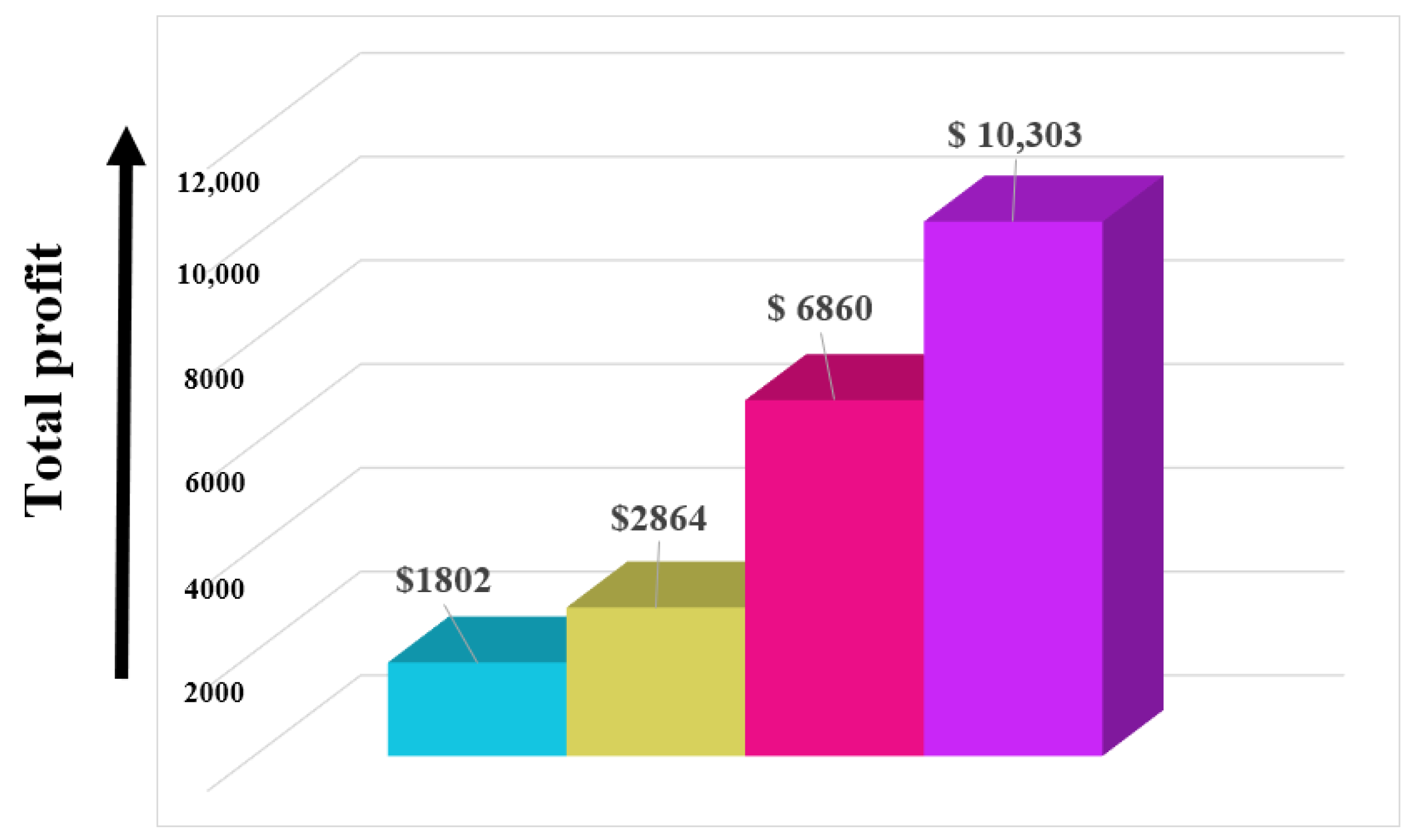
5.3. Comparison with Previous Literature

Compared to the existing literature, this research provided better results due to investment in reducing OC and a smart SSMD transportation policy.

Table 7. Comparison in total profit with existing literature.

	Pal et al. [17]	Dey et al. [34]	Dey et al. [5]	This Model
Ordering	NA	(constant)	NA	(reduced)
cost reduction	-	$200	-	$478
Production	NA	(constant)	(variable)	(variable)
rate	-	3200 unit	5994.25 unit	316.22 unit
Total Profit	2864 ($/cycle)	1802 ($/cycle)	6860 ($/cycle)	10,303 ($/cycle)

and Figure 6 are provided to clarify that the proposed model is beneficial for any industry. Table 7 indicates that a variable production rate and investment for reduction of OC is always beneficial for any SC system. Pal et al. [17] considered an SC system where demand depends on both quality and price; they solved the model for a centralized case and Stackelberg game policy, and the profit was $\$2864$ per cycle; quality was $0.71$; and also the production rate was constant. Dey et al. [34] developed an integrated model under selling-price-dependent demand and setup cost reduction, and the total system profit in their model was $\$1802$ per cycle. In this model, they considered a fixed OC as $\$200$.

Recently, Dey et al. [5] proposed a smart production model under the consideration of a variable production rate along with price and quality-sensitive demand. The system profit for their model was $\$6860$ per cycle. Interestingly, the total system profit in the present study is $10,303 per cycle which clearly indicates a much more profitable model. The profit is highly more beneficial in this current model due to the use of two discrete investments for the reduction in OC and setup cost, along with a continuous investment for increasing the process reliability through autonomation. This study also proves that ordering cost is reduced to $\$478$ through discrete investment. Thus, the present study is applicable for any industry due to the sustainability of the proposed model.

6. Sensitivity Analysis

The effect of different parametric values on the total supply chain profit is presented in the sensitivity analysis in

Table 8. Percentage change in total profit.

Parameters	Changes	$\mathrm{CPI}$	Parameters	Changes	$\mathrm{CPI}$
	(In%)	(In%)		(In%)	(In%)
$\alpha$	$+50$	$-0.20$	$\gamma$	$+50$	$-0.41$
	$+25$	$-0.10$		+25	$-0.21$
	$-25$	$+0.10$		$-25$	$+0.21$
	$-50$	$+0.26$		$-50$	$+0.41$
h	$+50$	$-0.41$	$h_V$	$+50$	$-0.82$
	$+25$	$-0.21$		+25	$-0.41$
	$-25$	$+0.20$		$-25$	$+0.41$
	$-50$	$+0.41$		$-50$	$+0.82$
S	$+50$	$-5.23$	$S_v$	$+50$	$-4.85$
	$+25$	$-1.89$		+25	$-2.43$
	$-25$	$+1.21$		$-25$	$+2.35$
	$-50$	$+6.14$		$-50$	$+4.53$
$\pi$	$+50$	$-2.69$	$I_{S_0}$	$+50$	$-1.24$
	$+25$	$-1.85$		+25	$-0.79$
	$-25$	$+1.67$		$-25$	$+0.90$
	$-50$	$+2.38$		$-50$	$+1.34$
$T_{C_{fb}}$	$+50$	$-0.11$	$V_b$	$+50$	$-0.99$
	$+25$	$-0.02$		+25	$-0.45$
	$-25$	$+0.06$		$-25$	$+0.66$
	$-50$	$+0.15$		$-50$	$+1.33$
$F_{CEB}$	$+50$	$-0.24$	$Y_b$	$+50$	$-0.25$
	$+25$	$-0.17$		+25	$-0.10$
	$-25$	$+0.15$		$-25$	$+0.06$
	$-50$	$+0.20$		$-50$	$+0.21$
$T_{f_{vb}}$	$+50$	$-0.16$	$T_{V_{vb}}$	$+50$	$-6.59$
	$+25$	$-0.06$		+25	$-2.54$
	$-25$	$+0.09$		$-25$	$+2.75$
	$-50$	$+0.12$		$-50$	$+6.45$
$F_{CV}$	$+50$	$-2.59$	$E_T$	$+50$	$-1.74$
	$+25$	$-1.57$		+25	$-0.86$
	$-25$	$+1.51$		$-25$	$+0.92$
	$-50$	$+2.68$		$-50$	$+1.45$

. Combined profit increase (CPI) $=\frac{Changeofprofit}{orginalprofit}\times 100\%$. From Table 8, the following conclusions could be made:

(i)

Holding cost significantly affects the total profit. An increase in holding cost always leads to increased total system cost, and system profit is reduced due to a high holding cost, which is more sensitive for the manufacturer compared to the retailer’s holding cost.

(ii)

Defective items in any imperfect production system always lead to less profit. This is the reason for incorporating autonomation to upgrade the reliability of the system.

(iii)

The fixed unit carbon emission cost for transportation and unit carbon emission costs for production are very sensitive in maximizing the profit. Reduction in those unit costs naturally increases the total system profit. Simultaneously, variable carbon emission cost per unit is slightly sensitive in the supply chain’s total profit. Similarly, carbon emission cost for the retailer due to transportation is also sensitive.

(iv)

More setup cost always leads to less profit. An investment is introduced to reduce the initial setup cost, which leads to a more significant profit gain.

(v)

Due to imperfect production processes, unit shortages occur, which are harmful to any production system, as clearly observed from the sensitivity analysis table. Small changes in shortage costs are very much effective for the total supply chain profit.

7. Managerial Insights

The industry managers can make several decisions based on the findings of this study as follows:

(i)

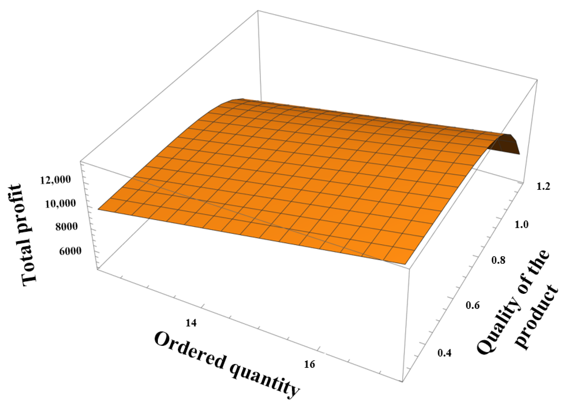
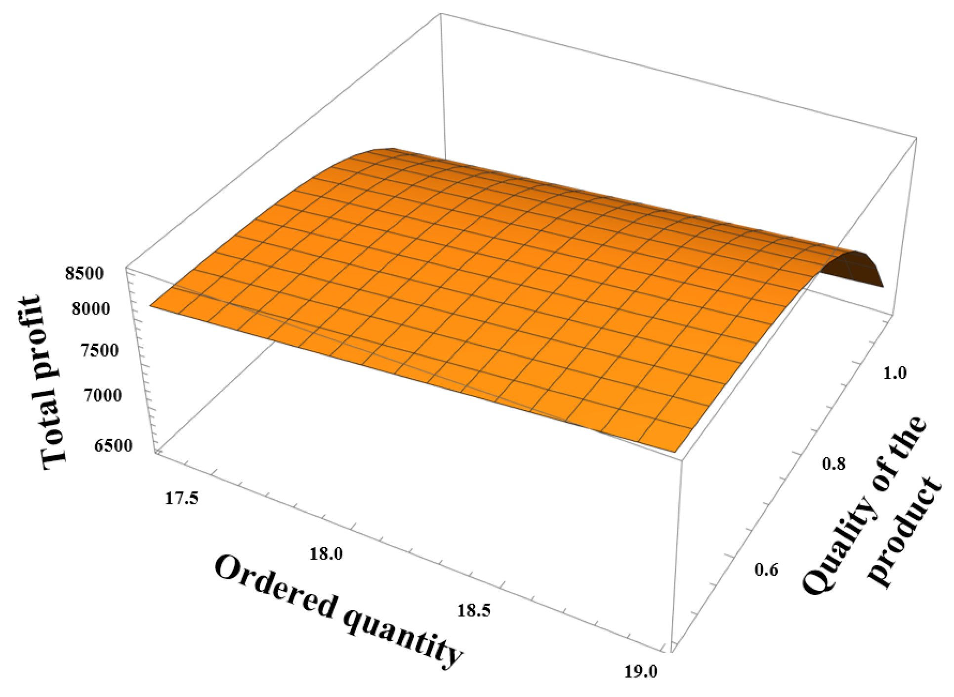
Product quality and selling price always enhance the demand for the product. Thus, managers of any industry can decide how much the selling price and quality of the products help optimize total system profit.

(ii)

The manager should maintain the investment to enhance the system’s reliability through autonomated inspection. Autonomated inspection for the production process can help perfectly detect the imperfection in the production process. Suppose the industry’s manager can control the movement of out-of-control from the in-control state of the production process. In that case, he can optimize the industry’s total profit by reducing the generation of the defective product. Simultaneously, managers can enhance the industry’s profit by managing the investment in setup and ordering costs.

(iii)

The industry managers may focus on their SCM performance by variable lead time. Because reduced lead time controls customer satisfaction as well as fulfills the market demand.

(iv)

Variable production rates are always beneficial for the industry to maintain its sustainability. Here, considerable unit production costs depend on development, tool/die, and environment-related costs. The investment for development cost helps the modification of product quality and helps to survive in competition. Eco-production helps to enhance environmental sustainability and improve total profit. Tool/die cost helps to reduce system failure and continues the production process. The industry manager can take this idea for their business strategy.

(v)

One other important finding is the variable safety factor. Variable safety factors largely control the holding cost based on fluctuating market demand. In the case of enormous demand, the holding cost is sometimes increased to stock the products, and in another point of low demand, the holding cost is reduced by limiting stock. Thus, making the right decision on safety stock is crucial. However, by the findings of this study, managers can make the right decision on safety stock.

8. Conclusions

Maximizing the total system’s profit while maintaining the sustainability of processes constitute a prominent challenge for any supply chain. A sustainable supply chain model for an environment friendly product with a single retailer and single manufacturer is presented here. We particularly focused on economic, environmental, and social benefits for a supply chain through different advanced strategies. While enhancing the sustainability of a supply chain, we optimize the manufacturer’s production quantity, production rate, and product quality. We additionally introduce investment for setup reduction and increase the process reliability through process autonomated inspection. We optimize the retailer’s safety factor, product selling price, and lead time along with investment for ordering cost reduction.

Selling price, quality-dependent demand, and variable production rate are also considered in the model for a more realistic representation. The classical optimization technique is utilized to solve the problem analytically. A proposition and improved algorithm are developed to obtain the optimal value of the decision variables and optimal profit of the supply chain. Numerical examples demonstrate that discrete investment played a significant role in reducing the ordering cost for the retailer up to $68\%$ as well as the setup cost for the manufacturer up to $22\%$. System reliability is also increased through an autonomation policy, which ultimately leads to an increased profit of a supply chain up to $64\%$. The SSMD policy increases the profit of the supply chain up to $34\%$.The supply chain profit is increased up to $16\%$ due to use of eco-production.

In this study, we only considered the offline channels for retailing, which is one of the limitations of the currently proposed model. Most retail channels run through dual channels (offline and online) (Guo et al. [48]). Thus, we will extend our study, including dual channels or multi-channel retailing. Another limitation of the presented model is its restriction to a two-player supply chain. The model can be extended by considering more players in a multi-echelon configuration (Cheng et al. [49]). Moreover, we will analyze the effect of SSMD in more detail compared with the multi-setup-multi-delivery (MSMD) (Sarkar et al. [18]) and multi-setup-multi-unequal-delivery (MSMUD) (Hota et al. [50]) strategies.

References

1. Garai, A.; Sarkar, B. Economically independent reverse logistics of customer-centric closed-loop supply chain for herbal medicines and biofuel. J. Clean Prod. 2022, 334, 129977. [Google Scholar] [CrossRef]
2. Seok, H.; Nof, S.Y.; Filip, F.G. Sustainability decision support system based on collaborative control theory. Annu. Rev. Control 2012, 36, 85–100. [Google Scholar] [CrossRef]
3. Sardar, S.K.; Sarkar, B.; Kim, B. Integrating Machine Learning, Radio Frequency Identification, and Consignment Policy for Reducing Unreliability in Smart Supply Chain Management. Processes 2021, 9, 247. [Google Scholar] [CrossRef]
4. Dumitrascu, O.; Dumitrascu, M.; Dobrotǎ, D. Performance Evaluation for a Sustainable Supply Chain Management System in the Automotive Industry Using Artificial Intelligence. Processes 2020, 8, 1384. [Google Scholar] [CrossRef]
5. Dey, B.K.; Pareek, S.; Tayyab, M.; Sarkar, B. Autonomation policy to control work-in-process inventory in a smart production system. Int. J. Prod. Res. 2021, 59, 1258–1280. [Google Scholar] [CrossRef]
6. Sarkar, M.; Chung, B.D. Flexible work-in-process production system in supply chain management under quality improvement. Int. J. Prod. Res. 2020, 58, 3821–3838. [Google Scholar] [CrossRef]
7. Dey, B.K.; Sarkar, B.; Sarkar, M.; Pareek, S. An integrated inventory model involving discrete setup cost reduction, variable safety factor, selling price dependent demand, and investment. Rairo-Oper. Res. 2019, 53, 39–57. [Google Scholar] [CrossRef]
8. Sarkar, B.; Chaudhuri, K.; Moon, I. Manufacturing setup cost reduction and quality improvement for the distribution free continuous-review inventory model with a service level constraint. J. Manuf. Syst. 2015, 34, 74–82. [Google Scholar] [CrossRef]
9. Sana, S. Price competition between green and non green products under corporate social responsible firm. J. Retail. Consum. Serv. 2020, 55, 102118. [Google Scholar] [CrossRef]
10. Mishra, U.; Wu, J.Z.; Sarkar, B. A sustainable production-inventory model for a controllable carbon emissions rate under shortages. J. Clean Prod. 2020, 256, 120268. [Google Scholar] [CrossRef]
11. Liu, K.; Li, W.; Jia, F.; Lan, Y. Optimal strategies of green product supply chains based on behaviour-based pricing. J. Clean Prod. 2022, 335, 130288. [Google Scholar] [CrossRef]
12. Sepehri, A.; Mishra, U.; Sarkar, B. A sustainable production-inventory model with imperfect quality under preservation technology and quality improvement investment. J. Clean Prod. 2022, 310, 127332. [Google Scholar] [CrossRef]
13. Sarkar, B.; Ullah, M.; Kim, N. Environmental and economic assessment of closed-loop supply chain with remanufacturing and returnable transport items. Comput. Ind. Eng. 2017, 111, 148–163. [Google Scholar] [CrossRef]
14. Sarkar, B.; Sarkar, M.; Ganguly, B.; Cárdenas-Barrón, L.E. Combined effects of carbon emission and production quality improvement for fixed lifetime products in a sustainable supply chain management. Int. J. Prod. Econ. 2021, 231, 107867. [Google Scholar] [CrossRef]
15. Taleizadeh, A.A.; Ahmadzadeh, K.; Ghavamifar, A. Designing an optimal sustainable supply chain system considering pricing decisions and resilience factors. J. Clean Prod. 2022, 332, 129895. [Google Scholar] [CrossRef]
16. Abdel-Basset, M.; Mohamed, R.; Sallam, K.; Elhoseny, M. A novel decision-making model for sustainable supply chain finance under uncertainty environment. J. Clean Prod. 2020, 269, 122324. [Google Scholar] [CrossRef]
17. Pal, B.; Sana, S.S.; Chaudhuri, K. Two-echelon manufacturer–retailer supply chain strategies with price, quality, and promotional effort sensitive demand. Int. Trans. Oper. Res. 2015, 22, 1071–1095. [Google Scholar] [CrossRef]
18. Sarkar, B.; Ahmed, W.; Kim, N. Joint effects of variable carbon emission cost and multi-delay-in-payments under single-setupmultiple-delivery policy in a global sustainable supply chain. J. Clean Prod. 2018, 185, 421–445. [Google Scholar] [CrossRef]
19. Bhuniya, S.; Pareek, S.; Sarkar, B. A supply chain model with service level constraints and strategies under uncertainty. Alex. Eng. J. 2021, 60, 6035–6052. [Google Scholar] [CrossRef]
20. Dey, B.K.; Bhuniya, S.; Sarkar, B. Involvement of controllable lead time and variable demand for a smart manufacturing system under a supply chain management. Expert Syst. Appl. 2021, 184, 115464. [Google Scholar] [CrossRef]
21. Sarkar, M.; Seo, Y.W. Renewable energy supply chain management with flexibility and automation in a production system. J. Clean Prod. 2021, 324, 129149. [Google Scholar] [CrossRef]
22. Kim, S.L.; Banerjee, A.; Burton, J. Production and delivery policies for enhanced supply chain partnerships. Int. J. Prod. Res. 2008, 46, 6207–6229. [Google Scholar] [CrossRef]
23. Chauhan, R.; Kumar, V.; Jana, T.K.; Majumder, A. A Modified Customization Strategy in a Dual-Channel Supply Chain Model with Price-Sensitive Stochastic Demand and Distribution-Free Approach. Math. Probl. Eng. 2021, 2021, 5549882. [Google Scholar] [CrossRef]
24. Nandra, R.; Majumder, A.; Mishra, M. A multi-retailer sustainable supply chain model with information sharing and quality deterioration. Rairo-Oper. Res. 2021, 55, S2773–S2794. [Google Scholar] [CrossRef]
25. Hong, Z.; Guo, X. Green product supply chain contracts considering environmental responsibilities. Omega 2019, 83, 155–166. [Google Scholar] [CrossRef]
26. Huang, C.K.; Cheng, T.; Kao, T.; Goyal, S. An integrated inventory model involving manufacturing setup cost reduction in compound Poisson process. Int. J. Prod. Res. 2011, 49, 1219–1228. [Google Scholar] [CrossRef]
27. Khouja, M.; Mehrez, A. Economic production lot size model with variable production rate and imperfect quality. J. Oper. Res. Soc. 1994, 45, 1405–1417. [Google Scholar]
28. Majumder, A.; Jaggi, C.K.; Sarkar, B. A multi-retailer supply chain model with backorder and variable production cost. Rairo-Oper. Res. 2018, 52, 943–954. [Google Scholar] [CrossRef]
29. Yu, W.; Han, R. The impact of pollution taxation on competitive green product choice strategies. Comput. Ind. Eng. 2019, 137, 106012. [Google Scholar] [CrossRef]
30. Sarkar, B.; Sana, S.S.; Chaudhuri, K. An imperfect production process for time varying demand with inflation and time value of money–an EMQ model. Expert Syst. Appl. 2011, 38, 13543–13548. [Google Scholar] [CrossRef]
31. Li, Q.; Zheng, S. Joint inventory replenishment and pricing control for systems with uncertain yield and demand. Oper. Res. 2006, 54, 696–705. [Google Scholar] [CrossRef]
32. Song, Y.; Wang, Y. Periodic review inventory systems with fixed order cost and uniform random yield. Eur. J. Oper. Res. 2017, 257, 106–117. [Google Scholar] [CrossRef]
33. Porteus, E.L. Optimal lot sizing, process quality improvement and setup cost reduction. Oper. Res. 1986, 34, 137–144. [Google Scholar] [CrossRef]
34. Dey, B.K.; Sarkar, B.; Pareek, S. A two-echelon supply chain management with setup time and cost reduction, quality improvement and variable production rate. Mathematics 2019, 7, 328. [Google Scholar] [CrossRef]
35. Wee, H.M.; Lee, M.C.; Jonas, C.; Wang, C.E. Optimal replenishment policy for a deteriorating green product: Life cycle costing analysis. Int. J. Prod. Econ. 2011, 133, 603–611. [Google Scholar] [CrossRef]
36. Su, J.C.; Wang, L.; Ho, J.C. The impacts of technology evolution on market structure for green products. Math. Comput. Model. 2012, 55, 1381–1400. [Google Scholar] [CrossRef]
37. Halat, K.; Hafezalkotob, A. Modeling carbon regulation policies in inventory decisions of a multi-stage green supply chain: A game theory approach. Comput. Ind. Eng. 2019, 128, 807–830. [Google Scholar] [CrossRef]
38. Darvish, M.; Archetti, C.; Coelho, L.C. Trade-offs between environmental and economic performance in production and inventoryrouting problems. Int. J. Prod. Econ. 2019, 217, 269–280. [Google Scholar] [CrossRef]
39. Ahmadini, A.A.H.; Modibbo, U.M.; Shaikh, A.A.; Ali, I. Multi-objective optimization modelling of sustainable green supply chain in inventory and production management. Alex. Eng. J. 2021, 60, 5129–5146. [Google Scholar] [CrossRef]
40. Becerra, P.; Mula, J.; Sanchis, R. Green supply chain quantitative models for sustainable inventory management: A review. J. Clean Prod. 2021, 328, 129544. [Google Scholar] [CrossRef]
41. Tang, S.; Wang, W.; Zhou, G. Remanufacturing in a competitive market: A closed-loop supply chain in a Stackelberg game framework. Expert Syst. Appl. 2020, 161, 113655. [Google Scholar] [CrossRef]
42. Sarkar, B.; Bhunia, S. A sustainable flexible manufacturing–remanufacturing model with improved service and green investment under variable demand. Expert Syst. Appl. 2022, 202, 117154. [Google Scholar] [CrossRef]
43. Kim, S.L.; Ha, D. A JIT lot-splitting model for supply chain management: Enhancing buyer–supplier linkage. Int. J. Prod. Econ. 2003, 86, 1–10. [Google Scholar] [CrossRef]
44. Wang, S.; Sarker, B.R. An assembly-type supply chain system controlled by kanbans under a just-in-time delivery policy. Eur. J. Oper. Res. 2005, 162, 153–172. [Google Scholar] [CrossRef]
45. Bhuniya, S.; Pareek, S.; Sarkar, B.; Sett, B. A Smart Production Process for the Optimum Energy Consumption with Maintenance Policy under a Supply Chain Management. Processes 2021, 9, 19. [Google Scholar] [CrossRef]
46. Ben-Said, A.; Moukrim, A.; Guibadj, R.N.; Verny, J. Using decomposition-based multi-objective algorithm to solve Selective Pickup and Delivery Problems with Time Windows. Comput. Oper. Res. 2022, 145, 105867. [Google Scholar] [CrossRef]
47. Tiwari, S.; Kazemi, N.; Modak, N.M.; Cárdenas-Barrón, L.E.; Sarkar, S. The effect of human errors on an integrated stochastic supply chain model with setup cost reduction and backorder price discount. Int. J. Prod. Econ. 2020, 226, 107643. [Google Scholar] [CrossRef]
48. Guo, X.; Liu, W.; Zhang, T. Pricing and ordering decisions for the supply chain integrating of online and offline channels. Environ. Dev. Sustain. 2022, 1–25, in press. [Google Scholar] [CrossRef]
49. Cheng, R.; Duan, Y.; Zhang, J.; Ke, H. Impacts of store-brand introduction on a multiple-echelon supply chain. Eur. J. Oper. Res. 2022, 292, 652–662. [Google Scholar] [CrossRef]
50. Hota, S.K.; Sarkar, B.; Ghosh, S.K. Effects of unequal lot size and variable transportation in unreliable supply chain management. Mathematics 2020, 8, 357. [Google Scholar] [CrossRef] [Green Version]
Figure 1. Enhancement of three pillars of sustainability in this study.
Processes 10 01775 g001
Figure 2. Selling price and quality depended demand pattern.
Processes 10 01775 g002
Figure 3. Inventory level for the retailer and manufacturer.
Processes 10 01775 g003
Figure 4. Total profit with respect to ordering quantity and quality of the product.
Processes 10 01775 g004
Figure 5. Total profit with respect to ordering quantity and quality of the product under fixed production rate.
Processes 10 01775 g005
Figure 6. Graphical representation of the comparison of total profit with Dey et al. [34], Pal et al. [17], and Dey et al. [5].
Processes 10 01775 g006