Motion Planning of an Inchworm Robot Based on Improved Adaptive PSO

Abstract

Focusing on the motion energy consumption of a self-developed inchworm robot’s peristaltic gait, based on the “error tracking” of cubic polynomial programming in Cartesian space and seventh polynomial programming in joint space, we propose an optimal motion planning method of energy consumption considering both kinematic and dynamic constraints. Firstly, we offer a mathematical description of the energy consumption and space curve similarity operator. Secondly, we describe the mathematical models of the robot trajectory and path that were established in terms of their dynamics and kinematics. Then, we propose a motion planning method based on improved adaptive particle swarm optimization (PSO) to accelerate the convergence speed of the algorithm and ensure the accuracy of the model calculation. Finally, we outline the simulation test carried out to measure the inchworm-like robot’s creeping gait. The results show that the motion path obtained by using the planning method proposed in this paper is the one with the least energy consumption by the robot among all the comparison paths. Moreover, compared with other algorithms, it was found that the result obtained by using the algorithm proposed in this paper is the one with the shortest solution time and the lowest energy consumption under the same iteration times. The calculation results verify the feasibility and effectiveness of the planning method.

1. Introduction

“Made in China 2025” is an action program that indicates that green manufacturing is set to be the future development trend of China’s manufacturing industry [1]. At the same time, artificial intelligence fields such as robotics are booming at present. In order to meet the needs of the times [2], reducing energy consumption as much as possible is an important goal of robot design. Therefore, this paper mainly explores how to minimize energy consumption in the process of robot movement, which, in essence, involves the optimal motion planning of the robot energy consumption from the starting point to the target point [3].

The geometrid-like robot was designed according to the geometrid, being a creature in nature. Its trunk is roughly the shape of an arched bridge and its posture is flexible. It can crawl in different environments. Its movement mode is peristalsis, crawling forward by means of adsorption at both ends and an extension of the middle joint, as shown in the Figure 1. For this paper, the model of the robot entity was constructed in order to study the energy consumption of the robot’s creeping gait. Figure 2 is a schematic diagram of the robot crawling.

At present, the main solution to the problem of robot motion planning in academic circles is to decompose it into sub-problems: The first sub-problem is path planning, which involves solving the effective path connecting two points in cartesian space based on the kinematic level, when we know the starting point and target point. Thus, Song, B. and Wang, Z. [4] suggested smooth path planning based on the improved algorithm of the continuous high-degree Bezier curve; Zhou, M. and Wang, Z. [5] suggested multi-objective path planning based on the improved GWO-WOA method; and Wang, J. and Chi, W. [6] suggested the shortest path planning based on neural network RRT* learning. The second sub-problem is path tracking, in the case where the robot path has been established, and the trajectory of the robot on the path is solved in joint space based on the dynamic level. For example, Zhang, T. and Zhang, M. [7] proposed an input shaping algorithm to replace the acceleration constraint in order to obtain a time-optimal smooth trajectory; Chai, R. and Tsourdos, A. [8] combined the real-time re-entry trajectory planning method of fuzzy multi-objective transcription and the deep neural network; and Shen, P. and Zhang, X. [9] based their method on torque and speed constraints, aiming at the optimality and completeness of algorithm time.

However, such methods also divide the motion planning problem into two parts and do not integrate the sub-problems well. Because solutions to path tracking need to be based on the solved kinematics of path planning, if path tracking is not considered in the process of solving the path planning, it is likely that the path will not meet the dynamic constraints; thus, the solving of path planning also needs to be based on the existing dynamics of path tracking. Therefore, path planning and path tracking go hand in hand, and the question of how to combine path planning and path tracking effectively is the key to solving the motion planning. For example, Jiang, L. and Guan, Y.S, [10], based on kinematic and dynamic constraints, used the lattice point search method to solve the optimal energy consumption, while Everett, M. and Yu, F.C. [11] proposed a motion planning method of dynamic decision for a mobile robot based on deep reinforcement learning. Due to the constraints, such as the combination of kinematics and dynamics, to solving the problem, it can be easily transformed into finding extremum under high dimensional nonlinear constraints. Therefore, it is difficult to apply traditional algorithms, such as the gradient descent method, to solve such problems, because the model is too complex and the objective function is mostly implicit, and the solution easily falls into the local optimal. For the resolution of this phenomenon, the academic community usually adopts heuristic algorithms, such as particle swarm optimization (PSO) [12], the genetic algorithm (GA) [13], Tabu search (TS) [14], Cuckoo search (CS) [15], and Beetle Antennae search (BAS) [16]. While PSO is widely used because it is not dependent on the problem information, has a strong universality and simple principle, is easy to implement, and has less adjustment parameters and other advantages, it still restricts the global search and local search ability because of the inertial weight operator in the algorithm. Therefore, it has become a focus of research. Inspired by the activation function of the neural network, this paper adopts the methods of self-adaptive adjustment of the function and setting the taboo area to solve this problem, so as to improve the convergence speed of the algorithm and ensure the accuracy of the model calculation.

In this paper, we study the energy consumption of an inchworm robot in a peristaltic gait of motion. Considering the kinematic and dynamic constraints of the robot and taking the minimum energy consumption as the optimization goal, we attempted to solve the optimized trajectory of the robot based on improved adaptive PSO.

The main contributions of this paper are as follows:

(1)

Based on “error tracking” of the cubic polynomial programming in Cartesian space and seventh polynomial programming in joint space, we propose an optimal motion planning method for energy consumption, considering both kinematic and dynamic constraints.

(2)

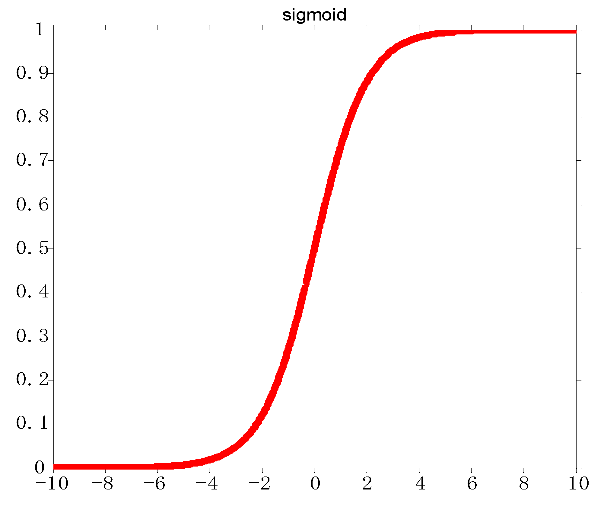
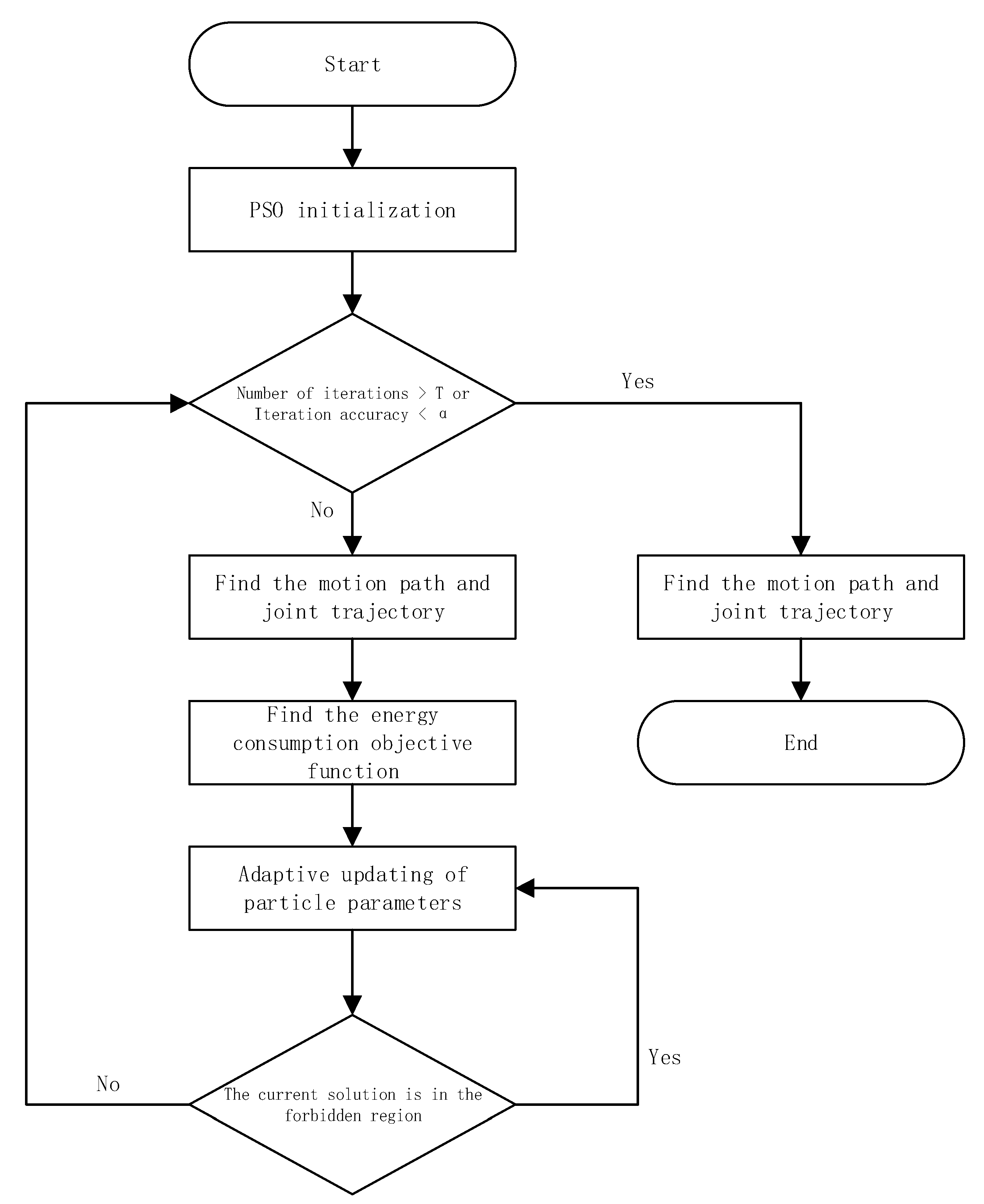
Based on the optimal energy consumption model, we propose an improved adaptive PSO algorithm using the function of the sigmoid adaptive to adjust the inertia weight operator and set the tabu region.

This paper is organized as follows. Section 2 establishes the robot’s indexes at the levels of its kinematics and dynamics, respectively. Section 3 describes the performance of the modeling and solving based on the improved adaptive PSO. Section 4 describes the performance of the simulation verification of the feasibility and effectiveness of the algorithm. The last section concludes this paper.

2. Motion Energy Consumption of the Inchworm-Mimicking Robot and Mathematical Description of the Spatial Curve Similarity Operator

2.1. Energy Consumption of Motion

If the robot is composed of L joints in series, the dynamics expression can be obtained by taking the derivative of the Lagrange equation [17]:

$$\{\begin{array}{l}{\tau }^i={\displaystyle \sum _{j=1}^{\mathrm{L}}{D}^{ij}{\ddot{q}}^j}+{\displaystyle \sum _{j=1}^{\mathrm{L}}{\displaystyle \sum _{k=1}^{\mathrm{L}}{D}^{ijk}}}{\dot{q}}^j{\dot{q}}^k+G^i\\ D^{ij}={\displaystyle \sum _{p=\max \left\{i,j\right\}}^{\mathrm{L}}tr\left(\frac{\partial T_0^p}{\partial q^j}{J}_p{\left(\frac{\partial T_0^p}{\partial q^i}\right)}^{\mathrm{T}}\right)}\\ D^{ijk}={\displaystyle \sum _{p=\max \left\{i,j\right\}}^{\mathrm{L}}tr\left(\frac{{\partial }^2{T}_0^p}{\partial q^j\partial q^k}{J}_p{\left(\frac{\partial T_0^p}{\partial q^j}\right)}^{\mathrm{T}}\right)}\\ \hspace{1em}\hspace{1em}=\frac{1}{2}\left(\frac{\partial D^{ij}}{\partial q^k}+\frac{\partial D^{ik}}{\partial q^j}-\frac{\partial D^{kj}}{\partial q^i}\right)\\ G^i={\displaystyle \sum _{p=i}^{\mathrm{L}}\left(-m_p{g}^{\mathrm{T}}\left(\frac{\partial T_0^p}{\partial q^j}{\overline{r}}_p\right)\right)}\\ T_{i-1}^i=\left(\begin{array}{cccc}\cos {\theta }_i& -\sin {\theta }_i\cos {\alpha }_i& \sin {\theta }_i\sin {\alpha }_i& a_i\cos {\theta }_i\\ \sin {\theta }_i& \cos {\theta }_i\cos {\alpha }_i& -\cos {\theta }_i\sin {\alpha }_i& a_i\sin {\theta }_i\\ 0& \sin {\alpha }_i& \cos {\alpha }_i& d_i\\ 0& 0& 0& 1\end{array}\right)\\ J_i=(\begin{array}{cc}\frac{1}{2}\left(-I_{ixx}+I_{iyy}+I_{izz}\right)& I_{ixy}\\ I_{ixy}& \frac{1}{2}\left(I_{ixx}-I_{iyy}+I_{izz}\right)\\ I_{ixz}& I_{iyz}\\ m_i{\overline{x}}_i& m_i{\overline{y}}_i\end{array}\\ \hspace{1em}\hspace{1em}\begin{array}{cc}{I}_{ixy}& m_i{\overline{x}}_i\\ I_{iyz}& m_i{\overline{y}}_i\\ \frac{1}{2}\left(I_{ixx}+I_{iyy}-I_{izz}\right)& m_i{\overline{z}}_i\\ m_i{\overline{z}}_i& m_i\end{array})\end{array}$$

(1)

Each joint moment of the robot can be composed of an inertia moment, a centrifugal force, a Coriolis force term and a gravity term. Before the two parts can be formed of every moment of the angular velocity and angular acceleration, in order to solve these two parts, the trajectories of the joint angular velocity and angular acceleration are required in advance. The third part of the gravity item is formed by the various joints, and its own gravity and center of mass offsets and centroid offset by the displacement of the joint trajectory. Thus, in order to obtain the torque of each joint, the first step is to calculate the angular displacement, angular velocity, and angular acceleration of each joint.

In the formula, the first part ${\displaystyle \sum _{j=1}^{\mathrm{L}}{D}^{ij}}{q}^j$ is the robot inertia term, the second part ${\displaystyle \sum _{j=1}^{\mathrm{L}}{\displaystyle \sum _{k=1}^{\mathrm{L}}{D}^{ijk}{\dot{q}}^j{\dot{q}}^k}}$ is the centrifugal force and Coriolis force term, and the third part $G^i$ is the gravity term. ${\tau }^i$, $q^i$, ${\dot{q}}^i$, and ${\ddot{q}}^i$ are the generalized moment, displacement, angular velocity, and angular acceleration of the $i$ joint, respectively; $g^{\mathrm{T}}$ is the gravity matrix; ${\overline{r}}_p$ is the position of the center of mass $p$ of the connecting rod; $T_{i-1}^i$ is the homogeneous coordinate transformation matrix of the $i$ coordinate system of the rod to the $i-1$ coordinate system of the rod; $a_i$ is the length of the $i$ rod; ${\alpha }_i$ is the torsion angle of the $i$ rod; ${\theta }_i$ is the $i$ joint angle; $d_i$ is the offset distance of the $i$ rod; $m_i$ is the mass of the $i$ rod; $\left({\overline{x}}_i, {\overline{y}}_i, {\overline{z}}_i\right)$ are the coordinates of the centroid of the $i$ bar; $I_{ixx}$, $I_{iyy}$, $I_{izz}$ are the mass moments of inertia of the $i$ bar; and $I_{ixy}$, $I_{iyz}$, $I_{ixz}$ are the products of inertia of the $i$ bar.

In actual motion, the motor provides energy for the robot to move from the starting point to the target point, but the total work performed by the robot is often not equal to the energy consumption of the motor. After consulting the literature [10], the total energy consumption of the motor in the process of robot movement can be roughly divided into the following parts:

1: The positive work effected by the motor on the robot is the energy consumption, when the joint torque is consistent with the direction of motion:

$$W={\displaystyle {\int }_{\dot{q}\left(t_{\mathrm{s}}\right)}^{\dot{q}\left(t_{\mathrm{e}}\right)}\tau \mathrm{d}\dot{q}},\tau \cdot \dot{q}>0$$

(2)

2: The negative work effected by the motor on the robot is the energy consumption, when the joint torque is opposite to the direction of motion:

$$W=\left|{\displaystyle {\int }_{\dot{q}\left(t_{\mathrm{s}}\right)}^{\dot{q}\left(t_{\mathrm{e}}\right)}\tau \mathrm{d}\dot{q}}\right|,\tau \cdot \dot{q}<0$$

(3)

3: The heat energy consumed by the motor is the energy consumption of the electric motor:

$$W={\displaystyle {\int }_{t_{\mathrm{s}}}^{t_{\mathrm{e}}}\left({\tau }^2/{\tau }_{\mathrm{Z}}\right) \mathrm{d}t},\tau \cdot \dot{q}=0$$

(4)

Due to the uncertainty of the heat loss, it is very challenging to solve the total energy consumption in detail. Therefore, Gregory, J. and Olivares, A. [18] proposed the adoption of a more intuitive and effective mathematical description of the robot’s motion energy consumption, as shown in the Equation (5):

$$W={\displaystyle {\int }_{t_{\mathrm{s}}}^{t_{\mathrm{e}}}{\tau }^2 \mathrm{d}t}$$

(5)

In the equation, $t_{\mathrm{s}}$ and $t_{\mathrm{e}}$ represent the start and end time of robot motion, respectively, $\dot{q}$ is the angular velocity of the joint motion, and ${\tau }_{\mathrm{Z}}$ is the impedance coefficient of the motor.

2.2. Space Curve Similarity Operator

Based on the “error tracking” model of cubic polynomial programming in Cartesian space and seventh polynomial programming in joint space, it is necessary to match the similarity between a certain motion path and the planned path in space, so that a space curve similarity operator can be defined. If there are two curves, ${\mathrm{L}}_1$ and ${\mathrm{L}}_2$, both of which consist of $N$ discrete points, the spatial similarity operator of these two curves can be expressed by the sum of the Euclidean distance squares of the points:

$$R={\displaystyle \sum _{i=1}^N\left({\left(X_i^{{\mathrm{L}}_1}-X_i^{{\mathrm{L}}_2}\right)}^2+{\left(Y_i^{{\mathrm{L}}_1}-Y_i^{{\mathrm{L}}_2}\right)}^2+{\left(Z_i^{{\mathrm{L}}_1}-Z_i^{{\mathrm{L}}_2}\right)}^2\right)}$$

(6)

In the equation, $\left(X_i^{{\mathrm{L}}_1}, Y_i^{{\mathrm{L}}_1}, Z_i^{{\mathrm{L}}_1}\right)$ is the spatial coordinate belonging to the $i$ point on the curve ${\mathrm{L}}_1$, and $\left(X_i^{{\mathrm{L}}_2}, Y_i^{{\mathrm{L}}_2}, Z_i^{{\mathrm{L}}_2}\right)$ is the spatial coordinate belonging to the $i$ point on the curve ${\mathrm{L}}_2$.

3. Motion Planning Method Based on the Optimal Energy Consumption

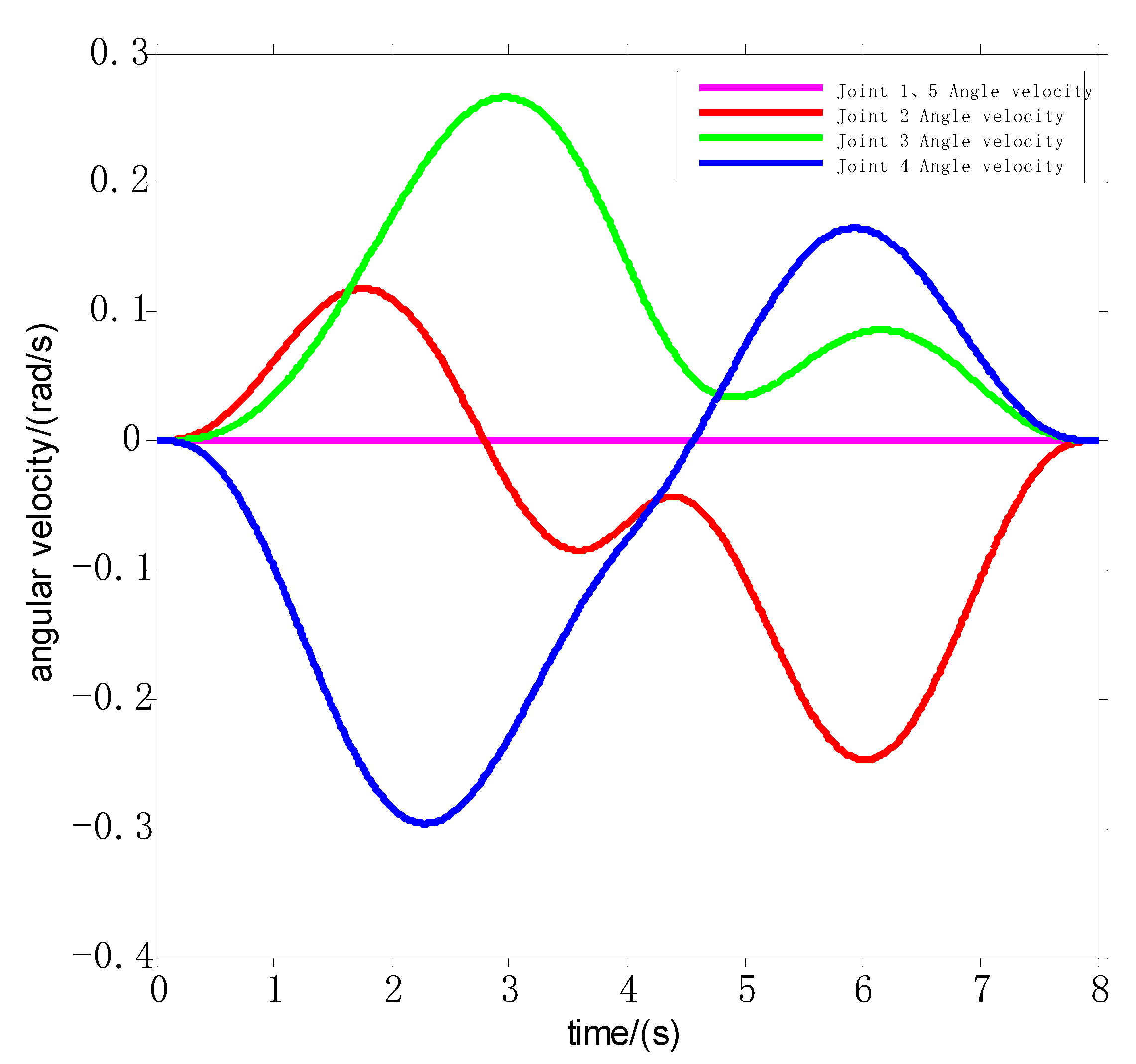
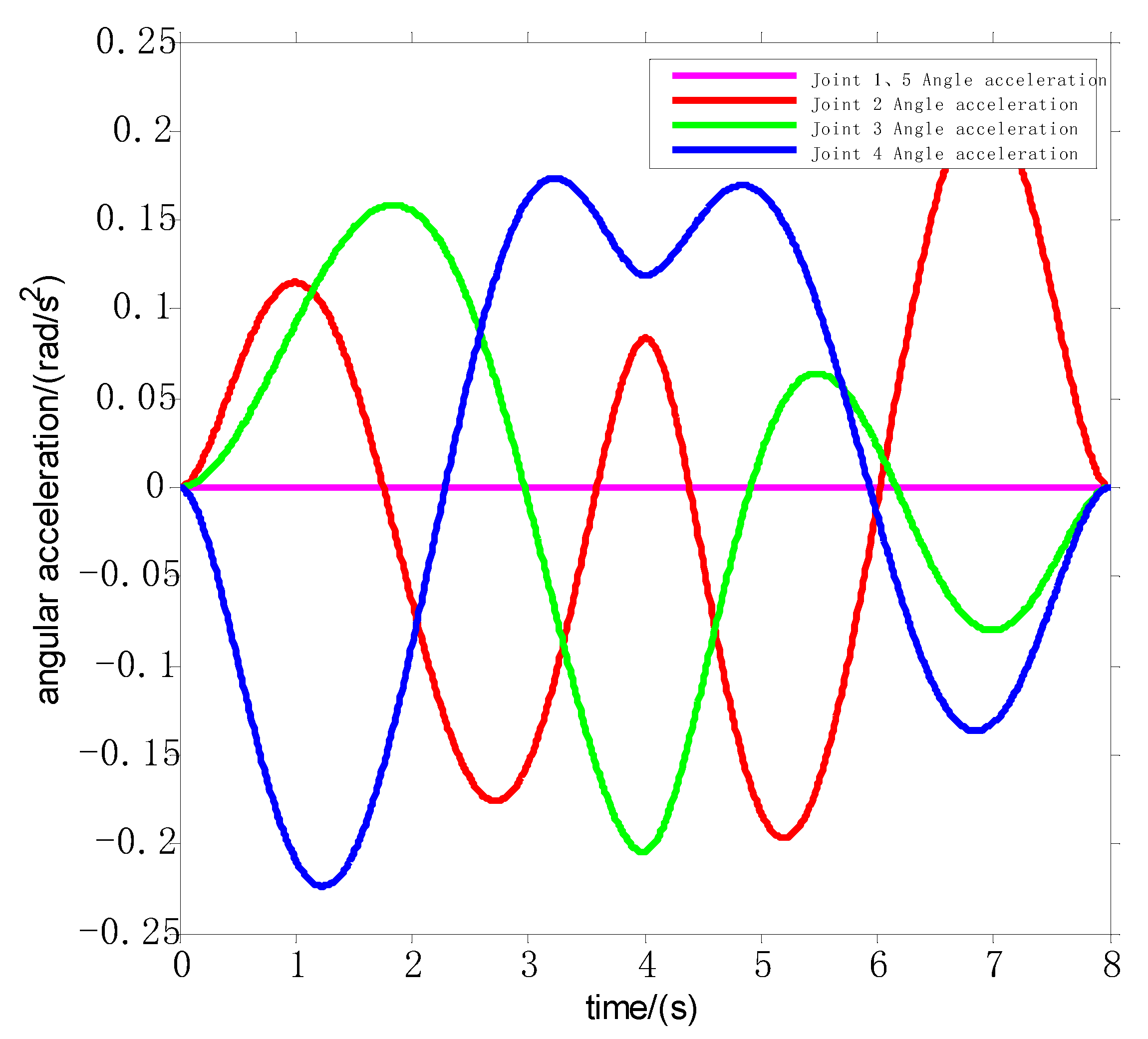
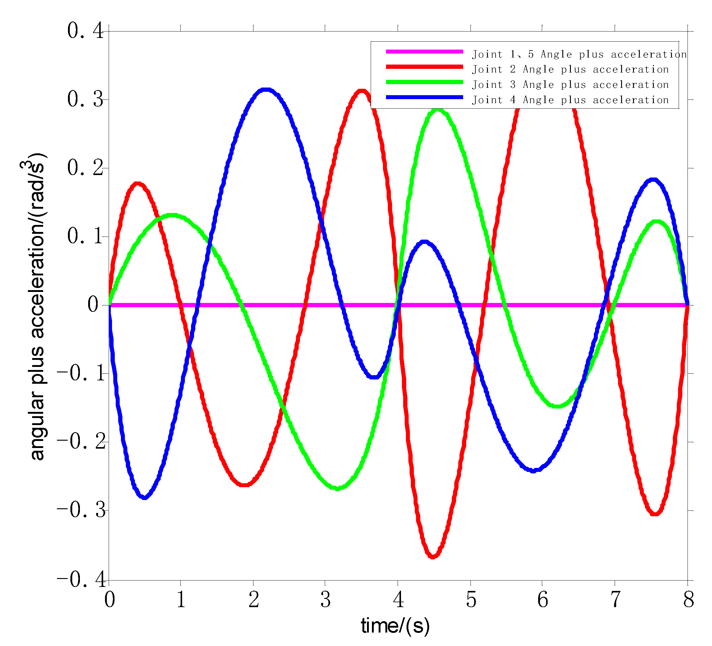
3.1. Continuous Trajectory Planning Based on Joint Space plus the Acceleration Curve

In actual motion, even if the starting point and target point states of all the joint spaces of the robot are determined, it is difficult to meet the requirements of the robot terminal motion path if a single polynomial programming method has been carried out for the joint space, respectively. Therefore, spline interpolation is generally carried out for the joint space in order to carry out the piecewise polynomial programming [19].

Multinomial spline interpolation: the function $S\left(t\right)\in C\left[t_{\mathrm{s}},t_{\mathrm{e}}\right]$, which is polynomial on each intercell $\left[t_j,t_{j+1}\right]$, where $t_{\mathrm{s}}=t_0<t_1<...<t_{n-1}<t_n=t_{\mathrm{e}}$ is a given node, is said to be a multinomial spline function on node $t_0,t_1,...,t_{n-1},t_n$.

In order to improve the smoothness of the motion and reduce the loss of the motor, it is necessary to constrain the change rate of the motor torque, and the motor torque is the driving force to produce the angular acceleration of the joint. Therefore, it is necessary to constrain the change rate of the angular acceleration of the joint—i.e., angle plus acceleration. In this study, we used piecewise cubic polynomial programming for the joint space of the robot in order to ensure that the joint space acceleration curve was smooth, so as to reduce the resonance of the motor [20].

Assume that the joint position of the ith joint at moments $t_j$ and $t_{j+1}$ is $q_j^i$ and $q_{j+1}^i$, the joint motion velocity is ${\dot{q}}_j^i$ and ${\dot{q}}_{j+1}^i$, the joint motion acceleration is ${\ddot{q}}_j^i$ and ${\ddot{q}}_{j+1}^i$, and the joint motion plus acceleration is ${\stackrel{⃛}{q}}_j^i$ and ${\stackrel{⃛}{q}}_{j+1}^i$. Thus, the complete boundary conditions of the robot joint space motion can be obtained, as shown in the Equation (7):

$$\{\begin{array}{l}{q}^i(t_j)=q_j^i,q^i(t_{j+1})=q_{j+1}^i\\ {\dot{q}}^i(t_j)={\dot{q}}_j^i,{\dot{q}}^i(t_{j+1})={\dot{q}}_{j+1}^i\\ {\ddot{q}}^i(t_j)={\ddot{q}}_j^i,{\ddot{q}}^i(t_{j+1})={\ddot{q}}_{j+1}^i\\ {\stackrel{⃛}{q}}^i(t_j)={\stackrel{⃛}{q}}_j^i,{\stackrel{⃛}{q}}^i(t_{j+1})={\stackrel{⃛}{q}}_{j+1}^i\end{array}$$

(7)

Since there are eight conditions, the polynomial needs to have at least eight coefficients in order to ensure a viable solution. Therefore, let the joint displacement polynomial in the interval be a seventh-degree polynomial, as shown in the Formula (8):

$$q^i(t)=a_0+a_{1}t+a_2{t}^2++a_3{t}^3+a_4{t}^4+a_5{t}^5+a_6{t}^6+a_7{t}^7$$

(8)

In order to solve the eight coefficients, such as $a_0,...,a_7$, the boundary conditions are expressed in matrix form, as shown in Formula (9), where the coefficients A and B are shown in Formulas (10) and (11), respectively:

$$A{\left[a_0,a_1,...,a_6,a_7\right]}^{\mathrm{T}}=B$$

(9)

$$A=\left[\begin{array}{llllllll} 1 & t_{\mathrm{j}}& t_{\mathrm{j}}^2& t_{\mathrm{j}}^3& t_{\mathrm{j}}^4& t_{\mathrm{j}}^5& t_{\mathrm{j}}^6& t_{\mathrm{j}}^7\\ 1 & t_{\mathrm{j}+1}^{}& t_{\mathrm{j}+1}^2& t_{\mathrm{j}+1}^3& t_{\mathrm{j}+1}^4& t_{\mathrm{j}+1}^5& t_{\mathrm{j}+1}^6& t_{\mathrm{j}+1}^7\\ & 1& 2t_{\mathrm{j}}& 3t_{\mathrm{j}}^2& 4t_{\mathrm{j}}^3& 5t_{\mathrm{j}}^4& 6t_{\mathrm{j}}^5& 7t_{\mathrm{j}}^6\\ & 1& 2t_{\mathrm{j}+1}& 3t_{\mathrm{j}+1}^2& 4t_{\mathrm{j}+1}^3& 5t_{\mathrm{j}+1}^4& 6t_{\mathrm{j}+1}^5& 7t_{\mathrm{j}+1}^6\\ & & 2& 6t_{\mathrm{j}}& 12t_{\mathrm{j}}^2& 20t_{\mathrm{j}}^3& 30t_{\mathrm{j}}^4& 42t_{\mathrm{j}}^5\\ & & 2& 6t_{\mathrm{j}+1}& 12t_{\mathrm{j}+1}^2& 20t_{\mathrm{j}+1}^3& 30t_{\mathrm{j}+1}^4& 42t_{\mathrm{j}+1}^5\\ & & & 6& {24}_{t\mathrm{j}}& 60t_{\mathrm{j}}^2& 120t_{\mathrm{j}}^3& 210t_{\mathrm{j}}^4\\ & & & 6& 24t_{\mathrm{j}+1}& 60t_{\mathrm{j}+1}^2& 120t_{\mathrm{j}+1}^3& 210t_{\mathrm{j}+1}^4\\ \end{array}\right]$$

(10)

$$B={\left[q_j^i,q_{j+1}^i,{\dot{q}}_j^i,{\dot{q}}_{j+1}^i,{\ddot{q}}_j^i,{\ddot{q}}_{j+1}^i,{\stackrel{⃛}{q}}_j^i,{\stackrel{⃛}{q}}_{j+1}^i\right]}^{\mathrm{T}}$$

(11)

If the time matrix $t_{\mathrm{all}}=\left[t_0,...,t_{j-1},t_j,...,t_n\right]$, as long as appropriate parameters such as $t_{\mathrm{all}}$ and $B$ are given, we can solve the eight parameters, such as $a_0,...,a_7$, so as to determine the displacement trajectory $q^i\left(t\right)$ of the ith joint. The velocity trajectory ${\dot{q}}^i\left(t\right)$, acceleration trajectory ${\ddot{q}}^i\left(t\right)$, and acceleration trajectory ${\stackrel{⃛}{q}}^i\left(t\right)$ can be obtained by obtaining the derivative successively.

Remark 1: 

Since the third equation has eight conditions, the polynomial needs to have at least eight coefficients in order to ensure a feasible solution. In addition, we discover by experimental simulation that the effect of the accuracy brought about by a higher-degree joint displacement polynomial is not significantly improved. Therefore, in order to simplify the complexity of the model, the joint displacement polynomial in this interval is set as a seventh-degree polynomial in order to ensure the calculation accuracy.

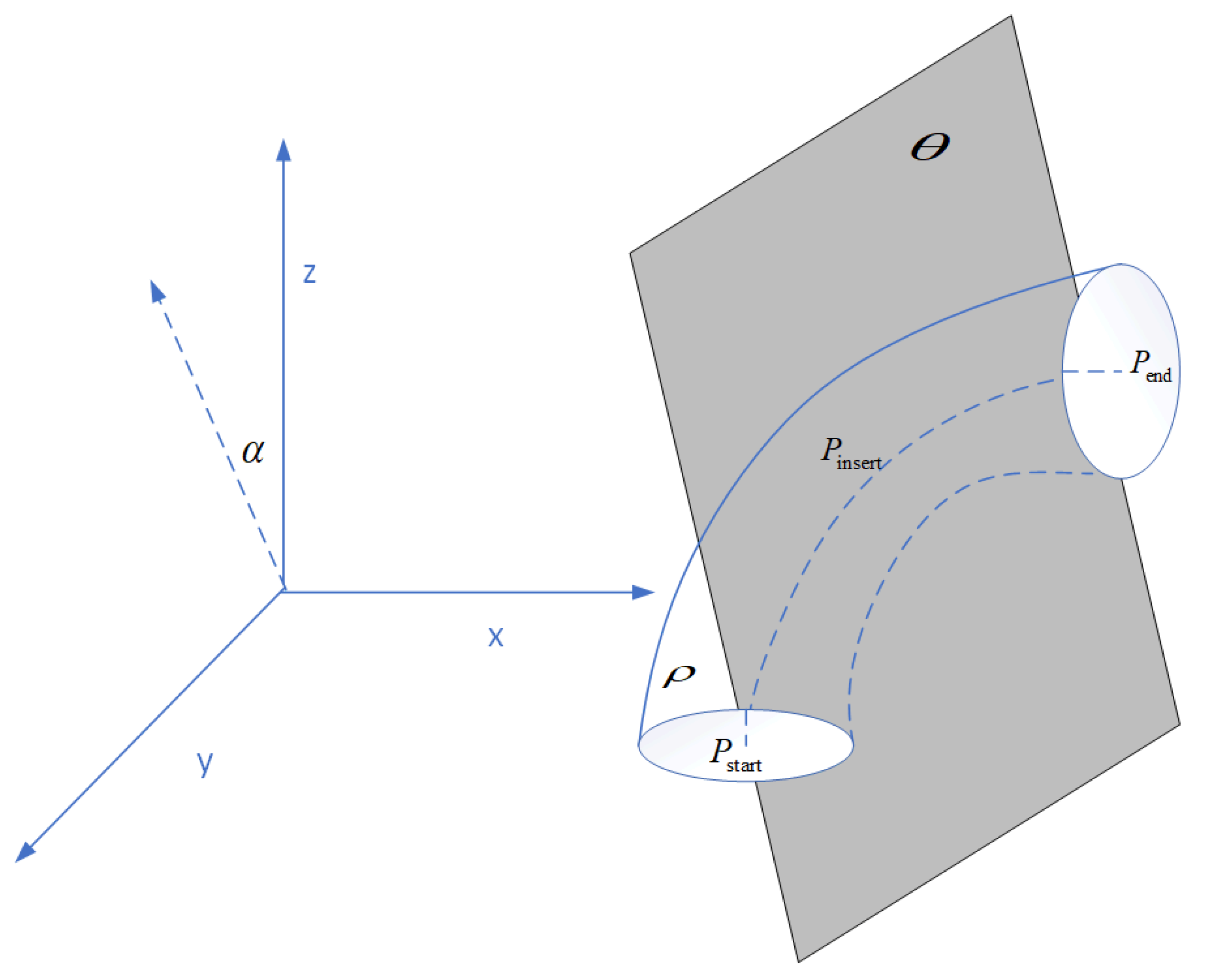
3.2. Path Planning Based on Cartesian Space Motion Curve Continuity

Given the starting point and ending point of the robot movement in the space, it is necessary to select an appropriate space curve to connect the points for the path of the robot movement. The curve consists of two features: 1: which surface the curve is on in the space; and 2: what the shape the curve on the surface has [21]. Since it is difficult to directly describe the shape of the surface and curve in the space, we first built a surface body based on a plane curve, taking the plane curve as the bus and using the curve similarity operator. The surface of the surface body was a spatial surface, and the curve similar to the bus shape on the space surface was a spatial curve.

Since three non-collinear points determine a plane, when $P_{\mathrm{start}}\left(X_{\mathrm{start}},Y_{\mathrm{start}},Z_{\mathrm{start}}\right)$ and $P_{\mathrm{end}}\left(X_{\mathrm{end}},Y_{\mathrm{end}},Z_{\mathrm{end}}\right)$ are known, if a suitable sample point $P_{\mathrm{insert}}\left(X_{\mathrm{insert}},Y_{\mathrm{insert}},Z_{\mathrm{insert}}\right)$ is chosen, the mixture product of three vectors formed by the property of space plane, where three points are zero, and the three-point equation of plane $\theta$ can be obtained as follows:

$$\left|\begin{array}{lll}x-x_{\mathrm{start}}& y-y_{\mathrm{start}}& z-z_{\mathrm{start}}\\ x_{\mathrm{insert}}-x_{\mathrm{start}}& y_{\mathrm{insert}}-y_{\mathrm{start}}& z_{\mathrm{insert}}-z_{\mathrm{start}}\\ x_{\mathrm{end}}-x_{\mathrm{start}}& y_{\mathrm{end}}-y_{\mathrm{start}}& z_{\mathrm{end}}-z_{\mathrm{start}}\end{array}\right|=0$$

(12)

For paths connecting the three points of the plane to make the curve smooth and continuous, cubic polynomials are needed as a minimum [22]. In the plane $\theta$, the position $p$ passing through the three points $P_{\mathrm{start}}$, $P_{\mathrm{insert}}$ and $P_{\mathrm{end}}$ is known. If the slope $\dot{p}$ of the path passing through the three points is determined, the complete path can be obtained by cubic polynomial interpolation.

Connect curves $P_{\mathrm{start}}{P}_{\mathrm{insert}}{P}_{\mathrm{end}}$ and define the similarity operator $R_{\max }$ of the spatial curves according to the similarity of the spatial curves based on Equation (6). If both curves are composed of $N$ points, then the maximum Euclidean distance of each point is $R_{\max }/N$ on average. The $N$ points of curve $P_{\mathrm{start}}{P}_{\mathrm{insert}}{P}_{\mathrm{end}}$ are taken as the center of the sphere, and $R_{\max }/N$ is taken as the radius, so that the $N$ sphere can be formed in the space. The surface of the feasible space $\rho$ is the surface of the $N$ spheres connected with the starting point $P_{\mathrm{start}}$ and the ending point $P_{\mathrm{end}}$. The curve $P_{\mathrm{start}}{P}_{\mathrm{insert}}{P}_{\mathrm{end}}$ is translated along the plane, intersecting the plane $\theta$ at an angle $\alpha$, and the space curve intersecting the surface $\rho$ is the feasible path of the robot motion. Figure 3 is an illustration of the space curve in Cartesian space.

Parameters $P_{\mathrm{insert}}$, $R_{\max }$, and $\alpha$ determine the position of the curve, and $\dot{p}$ determines the shape of the curve. If appropriate, $R_{\max }$, $\alpha$, and $\dot{p}$ are given, and the path of the robot in the feasible space can be obtained.

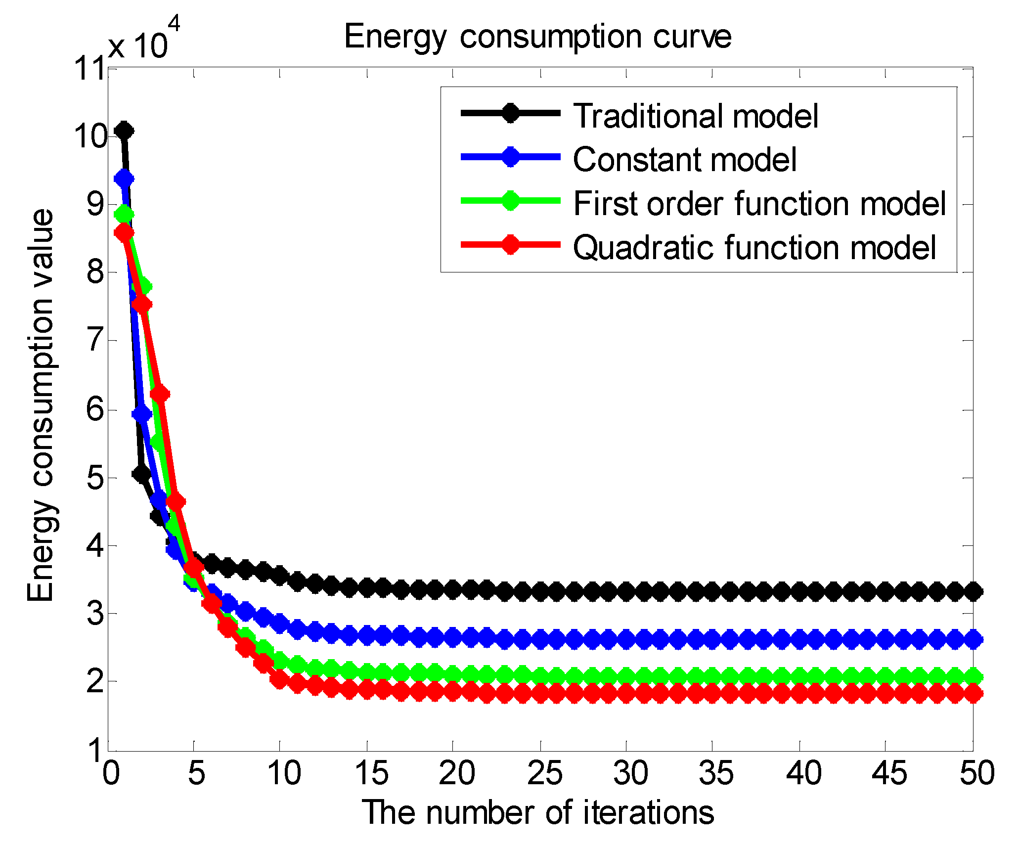
3.3. Trajectory Solving Based on Improved Adaptive PSO

After the joint trajectory and movement path of the robot are obtained, the torque of each joint can be obtained from Equations (1) and (9), as shown in Equation (13):

$$\begin{array}{l}{\tau }^i\left(t\right)=f\left(q^i(t),{\dot{q}}^i(t),{\ddot{q}}^i(t),{\stackrel{⃛}{q}}^i(t)\right)=g\left(t_{\mathrm{all}},q^i(t)\right)\\ \hspace{1em}\hspace{1em}={\displaystyle \sum _{j=1}^{n-1}g\left(t_{\mathrm{all}}\left(j\right),t_{\mathrm{all}}(j+1),q^i(t)\right)}\end{array}$$

(13)

where $f$ represents the implicit function of Newton–Euler dynamic recursion, and $g$ represents the function transformed by $t_{\mathrm{all}}$ and $q^i\left(t\right)$ for $q^i\left(t\right)$, ${\dot{q}}^i\left(t\right)$, ${\ddot{q}}^i\left(t\right)$ and ${\stackrel{⃛}{q}}^i\left(t\right)$. Thus, the energy consumption of the ith joint can be described as:

$$W^i={\displaystyle {\int }_0^T{\tau }^i{}^2}\mathrm{d}t={\displaystyle \sum _{j=0}^{n-1}{\displaystyle {\int }_{t_{\mathrm{all}}(j)}^{t_{\mathrm{all}}(j+1)}{g}^2\left(t_{\mathrm{all}}(j),t_{\mathrm{all}}(j+1),q^i(t)\right)\mathrm{d}t}}$$

(14)

Among these methods, when combining Cartesian space path planning and joint space trajectory planning, $q^i\left(t\right)$ can be described by $P_{\mathrm{insert}}$, $R_{\max }$, $\alpha$ and $\dot{p}$. Therefore, the solution model is finally transformed into:

$$\min {\displaystyle \sum _{i=1}^{\mathrm{L}}{\displaystyle \sum _{j=1}^{n-1}{\displaystyle {\int }_{t_{\mathrm{all}}(j)}^{t_{\mathrm{all}}(j+1)}{g}^2\left(t_{\mathrm{all}}(j),t_{\mathrm{all}}(j+1),P_{\mathrm{insert}},R_{\max },\alpha ,\dot{p}\right)\mathrm{d}t}}}$$

(15)

$$s.t\{\begin{array}{l}h\left(t_{\mathrm{all}}(j),t_{\mathrm{all}}(j+1),P_{\mathrm{insert}},R_{\max },\alpha ,\dot{p} \right)\ge {\tau }_{\mathrm{lb}}^i\\ h\left(t_{\mathrm{all}}(j),t_{\mathrm{all}}(j+1),P_{\mathrm{insert}},R_{\max },\alpha ,\dot{p} \right)\le {\tau }_{\mathrm{ub}}^i\\ P_{\mathrm{insert}}\in Q\\ R_{\max }\le d\\ 0\le \alpha \le 2\pi \\ \dot{p}\in \epsilon \\ q_{\mathrm{lb}}^i\le q^i\le q_{\mathrm{ub}}^i\\ {\dot{q}}_{\mathrm{lb}}^i\le {\dot{q}}^i\le {\dot{q}}_{\mathrm{ub}}^i\\ {\ddot{q}}_{\mathrm{lb}}^i\le {\ddot{q}}^i\le {\ddot{q}}_{\mathrm{ub}}^i\\ {\stackrel{⃛}{q}}_{\mathrm{lb}}^i\le {\stackrel{⃛}{q}}^i\le {\stackrel{⃛}{q}}_{\mathrm{ub}}^i\end{array}$$

(16)

where $Q$ is the workspace area of the robot, $d$ is a fixed distance coefficient, and $\epsilon$ is a real number. From the above model, it can be inferred that, if an appropriate $t_{\mathrm{all}}$ is selected during joint space trajectory planning, the whole solution process works to optimize the parameters of the path curve in Cartesian space.

In order to solve the minimum value of this objective function, traditional methods, such as the gradient descent method, have a fast convergence rate [23], but the objective function of this model is an implicit function, which makes it difficult to apply the gradient descent method. However, the PSO algorithm is widely used to solve this kind of model due to its advantages, such as the fact that it does not rely on problem information, its strong universality, simple principle, easy implementation, fewer adjustment parameters, etc. Therefore, in this study we adopted the PSO algorithm [24].

The PSO algorithm is a population $X=\left(x_1,...x_i,...x_M\right)$ composed of $M$ particles in a T-dimensional space. The position of the ith particle is $X_i=\left(x_{i1},...x_{iT}\right)$, the velocity of the ith particle is $V_i=\left(v_{i1},...v_{iT}\right)$, the global extreme value of the population is $B_w=\left(b_{w1},...b_{wT}\right)$, and the individual extreme value of the particle is $B_i=\left(b_{i1},...b_{iT}\right)$. Particle $x_i$ updates its speed and position as follows:

$$\{\begin{array}{l}{V}_i\left(k+1\right)=w{V}_i\left(k\right)+s_1{r}_1\left(k\right)\left(B_i\left(k\right)-X_i\left(k\right)\right)+s_2{r}_2\left(k\right)\left(B_w\left(k\right)-X_i\left(k\right)\right)\\ X_i\left(k+1\right)=X_i\left(k\right)+V_i\left(k+1\right)\end{array}$$

(17)

where, $i=1,...,M$, $k=1,...,T$, $i$ is the population size and $k$ is the number of evolution. $r_1$ and $r_2$ are random numbers distributed between $\left[0,1\right]$, $s_1$ and $s_2$ are individual learning factors and group learning factors, respectively, and $w$ is the inertial weight. When $w$ is large, the global search ability is strong, and when $w$ is small, the local search ability is strong. If the value is adjusted adaptively, the global search can be used first to cause the search space to converge in a certain region quickly, and then the local search can be used to obtain the high-precision solution.

Therefore, the question of how to define the inertial weight operator is related to the convergence speed and solving accuracy of the algorithm. Inspired by the neural network activation function, for this paper we adopted the sigmoid function to define the inertial weight operator [25], as shown in the Formula (18):

$$w\left(k\right)=\frac{1}{1+e^{-\left(h\left(k-1\right)-h\left(k\right)\right)/d}}$$

(18)

where the function $h$ is the fitness function, which is the objective function of this paper, as shown in Equation (12), and $d$ is the attenuation coefficient. The greatest feature of the w adaptive function proposed in this paper is the introduction of the objective function, which adapts the step size of the search by calculating the value of difference of the objective function to the input of the sigmoid function. When $h\left(k-1\right)-h\left(k\right)$ is greater, note that the algorithm is not searching the local optimal area, and there is a need to strengthen the global search ability. The w value is greater once $h\left(k-1\right)-h\left(k\right)$ becomes smaller, the specification has converged in a certain area, and there is a need to strengthen the local search ability. Thus, the w value is reduced by using the fast decay property of the sigmoid function. The function of the inertial weight operator is shown in Figure 4:

Because the objective function of the solution is complex, even after the inertia weight operator W is optimized, the solution will still fall into local optimization many times, resulting in a reduction in the efficiency of the solution. Therefore, it is necessary to further optimize the algorithm. For this reason, the tabu area in the algorithm is introduced [26], and the spatial complexity of the algorithm is exchanged for the time complexity in order to solve this problem.

The Tabu search (TS) algorithm is based on a local neighborhood search, where the taboos table is set to taboo some experienced operations, and contempt criteria are used to reward certain good states, and the global optimal solution is finally screened by comparison. The tabu area is the searched space in the tabu table. In this study, tabu area was set as the local optimal area obtained by the algorithm in the search process, so as to ensure the avoidance of this area in the subsequent search process and speed up the convergence of the algorithm.

In this study, the concept of the taboo region was defined as follows: Take the locally optimal solution $X_i=\left(x_{i1},...x_{iT}\right)$ as the geometric center of space, and the average length of step $\eta$ of n in the search process as the radius $r$. The feasible solution space satisfying Formula (19) is the taboo region:

$${\left(x-x_{i1}\right)}^2+...+{\left(x-x_{iT}\right)}^2\le r$$

(19)

According to the above description, after the algorithm converges in a certain region, the inertia weight operator decreases, and then the step size $\eta$ is also small, so that the step size $\eta$ must be small in a period of time before the algorithm searches for the local optimal solution, and then the radius $r$ depends on the number of steps $n$. When $n$ is too small, the tabu radius is too small to reflect the scale of the tabu area, leading to the insufficient convergence speed of the algorithm; when $n$ is too large, the tabu radius is too large, leading to the overwide coverage of the tabu area, leading to the reduction in the algorithm’s solution accuracy. The simulation results show that, when $n$ is 10, both the convergence speed and solution accuracy are considered.

To sum up, the algorithm flow for solving the model is shown in Figure 5:

4. Example of Imitated Inchworm Robot Movement Planning

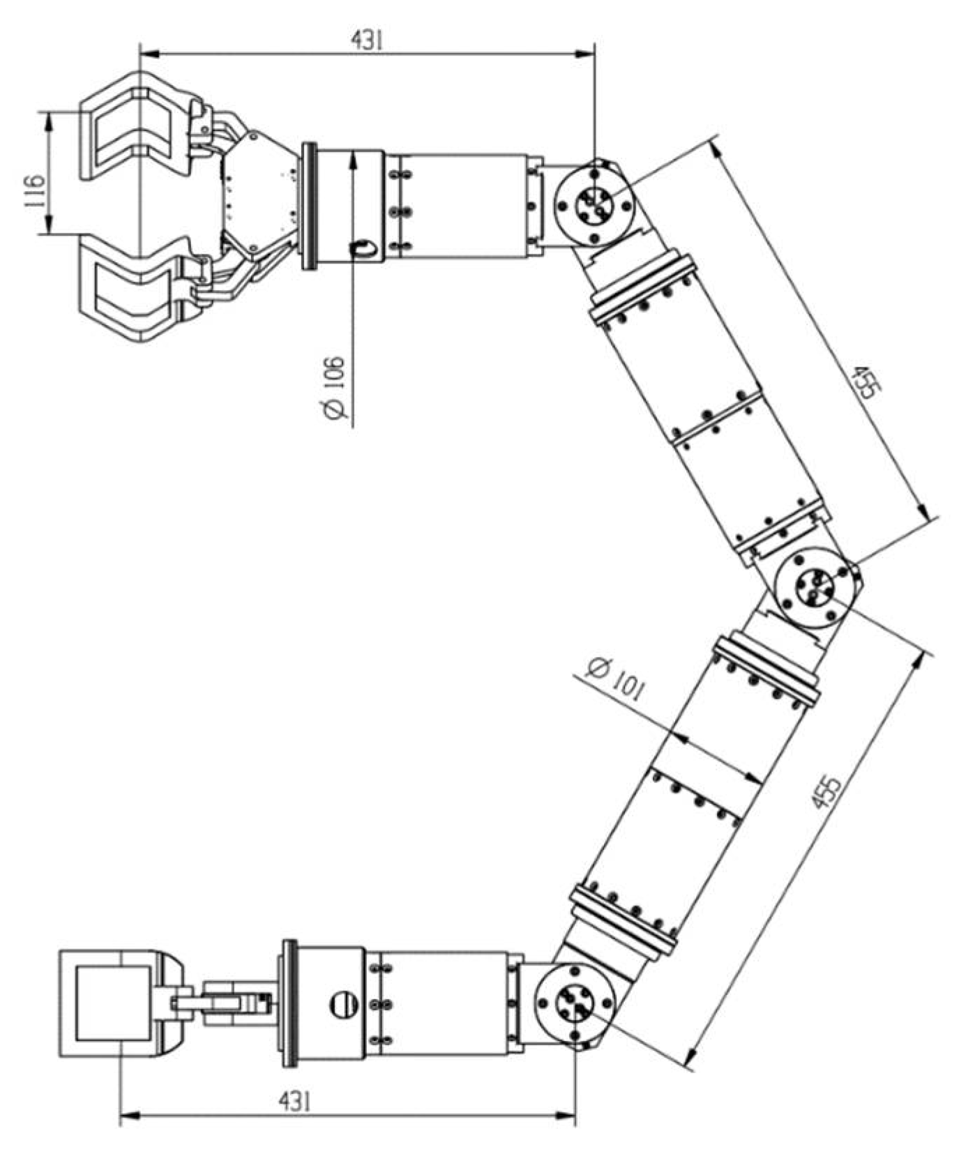
4.1. Dynamic Parameters of the Inchworm Robot Imitation

The robot was constructed adopting the modular design method. The upper and lower parts are completely symmetrical, with both ends being gripper modules, and the middle body part is composed of two joint modules. The joint module close to the gripper is marked as the I joint because its rotation direction and connecting rod axis overlap, and the middle joint module is marked as the T joint because its rotation direction and connecting rod axis are perpendicular. Figure 6 offers the parameter diagram of the robot.

According to the actual load capacity of the robot, its dynamic constraints are as shown in Equation (20):

$$\{\begin{array}{l}-134\mathrm{N}\cdot \mathrm{m}\le {\tau }^i\le 134\mathrm{N}\cdot \mathrm{m},i=1,...,5\\ -\pi \mathrm{rad}\le q^i\le \pi \mathrm{rad},i=1,...,5\\ -1.28\mathrm{rad}/\mathrm{s}\le {\dot{q}}^i\le 1.28\mathrm{rad}/\mathrm{s},i=1,...,5\\ -1.12\mathrm{rad}/{\mathrm{s}}^2\le {\ddot{q}}^i\le 1.12\mathrm{rad}/{\mathrm{s}}^2,i=1,...,5\\ -0.95{\mathrm{rad}/\mathrm{s}}^3\le {\stackrel{⃛}{q}}^i\le 0.95\mathrm{rad}/{\mathrm{s}}^3,i=1,...,5\end{array}$$

(20)

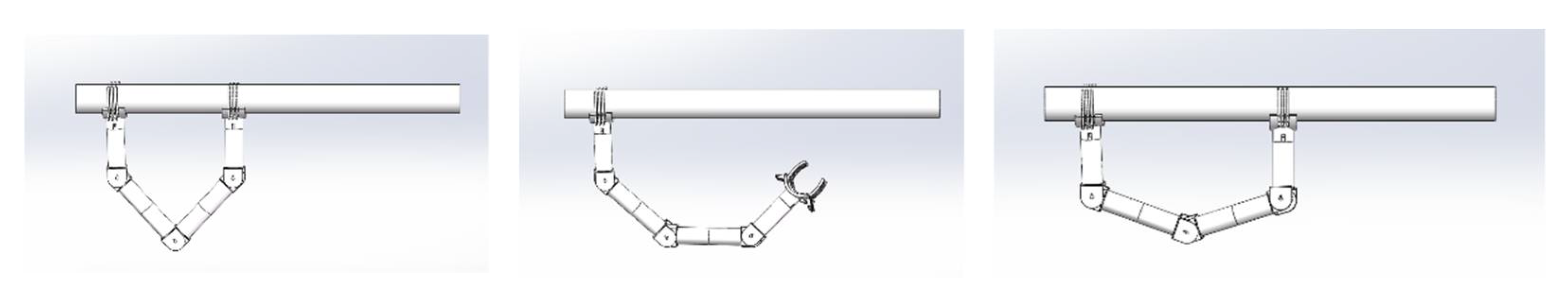
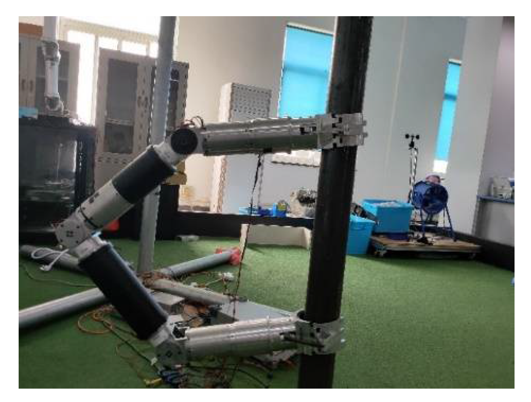
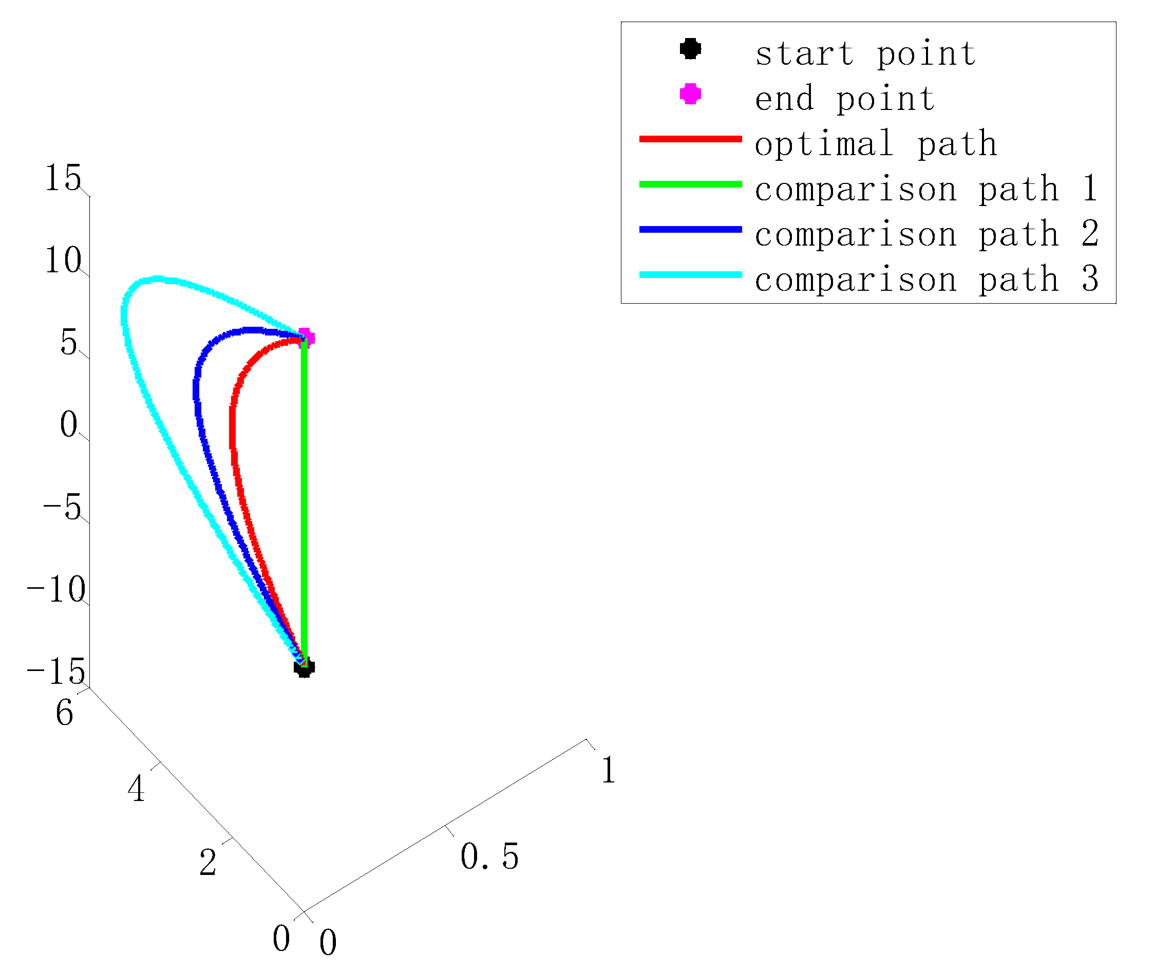
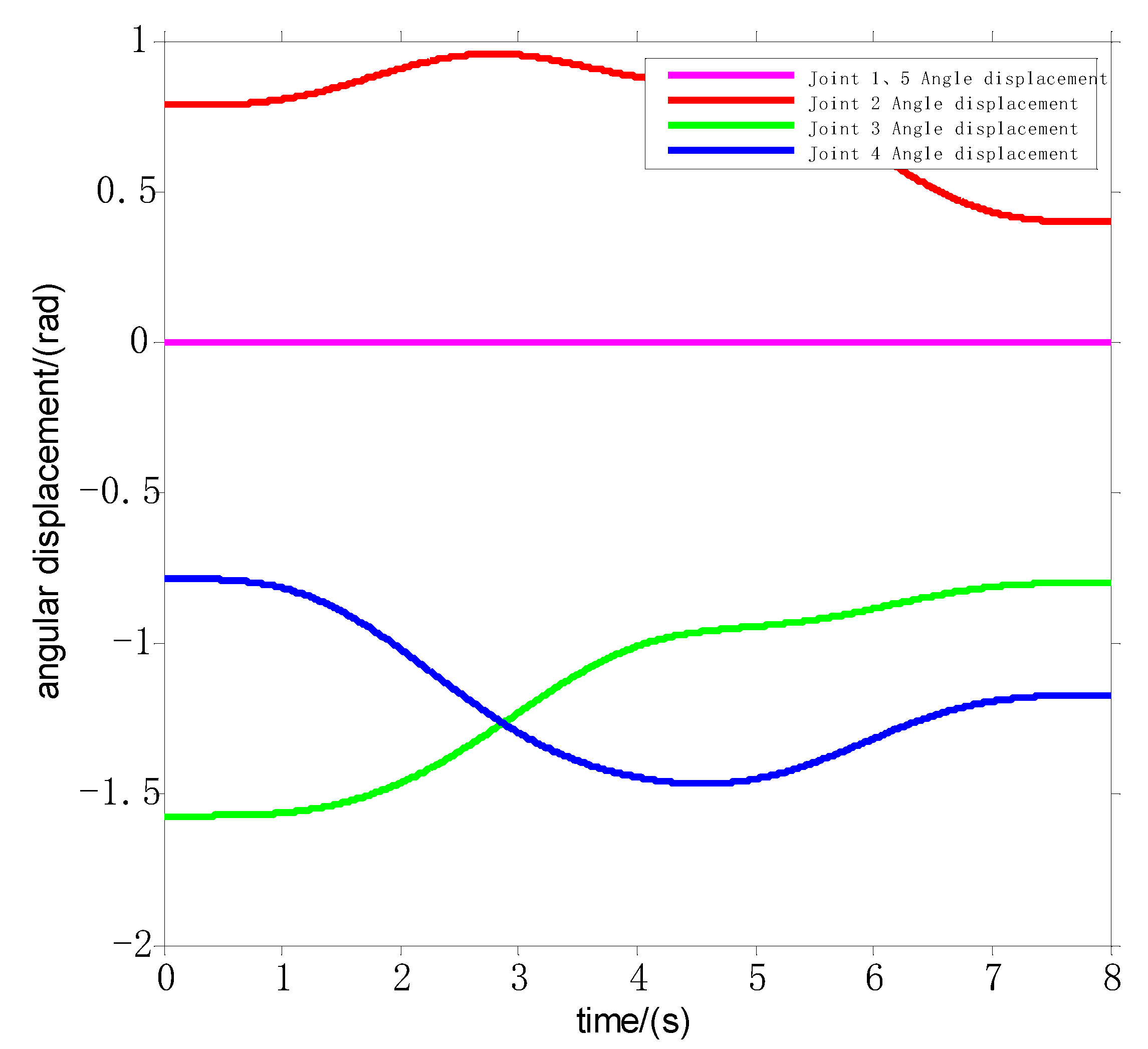
4.2. Simulation Experiment of the Inchworm Robot Climbing a Straight Bar

In order to verify the feasibility and effectiveness of the optimal motion planning method of energy consumption proposed here, we took the inchworm robot as the research object and had it carry out a straight bar climbing experiment in the Matlab simulation environment. The climbing scene is shown in Figure 7. The robot was required to climb from the starting position to the ending position on the vertical bar in space.

The optimal climbing path for the energy consumption, as obtained by the motion planning method proposed in this paper, is shown in Figure 8. In order to demonstrate the feasibility of the algorithm, three effective paths near and far from the optimal path were selected for comparative testing, which were respectively denoted as comparative path 1, 2, 3, with the parameters shown in

Table 1. Parameters of the different paths.

Path	Pinsert	Rmax	α	$\dot{\mathit{p}}$
Optimal path	(0, 5, 7.5)	5	0	(2.5, 0, 2.5)
Comparison path 1	(0, 0, 7.5)	5	0	(0, 0, 0)
Comparison path 2	(0, 10, 7.5)	5	0	(5, 0, 5)
Comparison path 3	(0, 15, 7.5)	5	0	(10, 0, 10)

.

Table 2. Comparison of the energy consumption levels of the different climbing paths on a straight rod.

Path	Movement Time/$\mathbf{S}$	Energy Consumption/(N2·m2·s)	Maximum Moment/(N·m)
Optimal path	8	1.97 $\times$ 104	97
Comparison path 1	8	2.28 $\times$ 104	100
Comparison path 2	8	2.06 $\times$ 104	106
Comparison path 3	8	2.66 $\times$ 104	128

shows the corresponding energy consumption and maximum torque values of these different paths in the same motion time. From the data available in the table, using the motion path obtained by the proposed planning method, we can observe that these all contrasted with the robot path with the least energy consumption, along with the angular displacement, angular velocity, angular acceleration, and angular plus acceleration curves of each joint during the robot’s climbing, which are shown in Figure 9, Figure 10, Figure 11 and Figure 12.

As shown in Figure 8, the angular displacement of each joint did not reach the maximum displacement, indicating that each joint works normally. As seen in Figure 9, Figure 10 and Figure 11, the angular velocity, angular acceleration, and angular acceleration of each joint did not exceed the upper limit of power of the motor itself, indicating that it can effectively provide the power demanded for the robot motion. All the curves in the figure are continuous and smooth, indicating that the joints were less impacted during the movement of the robot, and that the motor ran smoothly, which can extend the service life of the motor effectively.

5. Analysis and Discussion of the Model

In this paper, the inertial weight operator in the traditional PSO was combined with the sigmoid function, and the difference of the objective function $h\left(k-1\right)-h\left(k\right)$ divided by the attenuation coefficient $d$ of each iteration was taken as the input of the sigmoid function in order to achieve self-adaptation. When $h\left(k-1\right)-h\left(k\right)$ was large, it indicated that the algorithm had not searched the local optimal region, and the global search ability needed to be strengthened. At this time, the w value was large. Once $h\left(k-1\right)-h\left(k\right)$ became small, it indicated that it had converged in a certain region, and the local search ability needed to be strengthened. At this time, the w value could be reduced by using the fast decay of the sigmoid function. The purpose of introducing the attenuation coefficient $d$ was to smooth the input and prevent the over-fitting of the algorithm [27].

In this paper, in order to explore the attenuation coefficient d for the purpose of solving the model, in the same simulation environment, the initial population was set to 200, and we established the traditional PSO model without the attenuation coefficient $d$, the constant model with the maximum iteration number 50, the first-order function model with the iteration number K, and the quadratic function model with the iteration number K, respectively. The results are shown in Figure 13:

It can be seen from Figure 13 that the traditional model converged quickly in the early stage but tended to fall into the local optimum in the later stage, resulting in a low solution accuracy. After the introduction of the attenuation coefficient $d$, the convergence of the algorithm became slow in the early stage due to the existence of $d$, but the search accuracy was higher in the later stage, and it was easier to obtain the optimal solution. Moreover, $d$ was the lowest energy consumption obtained by the quadratic function model, indicating that the attenuation coefficient $d$ based on the solution model in this paper was more consistent with the quadratic function model with the number of iterations $k$.

In order to demonstrate the effectiveness of the algorithm, the genetic algorithm (GA), Tabu search (TS), Cuckoo search (CS), and Beetle Antennae search (BAS) algorithms were selected to conduct 20 comparative calculations with the improved adaptive particle swarm optimization (PSO) proposed in this paper, and the average solution time and minimum energy consumption indexes are shown in

Table 3. The average solving time of the different algorithms compared with the minimum energy consumption index.

Algorithm	Number of Iterations/Time	Energy Consumption/(N2·m2·s)	Solution Time/s
Improved adaptive PSO	50	1.97 $\times$ 104	168
GA	50	2.86 $\times$ 104	288
TS	50	2.68 $\times$ 104	246
CS	50	2.44 $\times$ 104	229
BAS	50	2.51 $\times$ 104	235

:

It can be seen from the data in the table that the results obtained using the algorithm proposed in this paper showed the shortest solving time and the lowest energy consumption in the same number of iterations among all the comparison algorithms.

6. Conclusions

In this paper, the optimal energy consumption of an inchworm robot was studied by testing the peristaltic gait of the inchworm robot. Firstly, an intuitive and effective method was used to describe the total energy consumption of the robot climbing and the spatial curve similarity operator. Secondly, a motion planning method based on the optimal energy consumption for climbing was formulated, and the motion planning method was made up of three parts: the first part was based on the trajectory planning of the joint space and continuous acceleration curve, the second part was based on the cartesian space motion curve continuous path planning, and the third part was based on the improved adaptive PSO to obtain the solution of the model. The most important feature of this method is that the kinematic and dynamic constraints of the robot are organically combined, and the complexity of the solution is reduced through the intuitive building of the model and the effective algorithm optimization. Finally, the actual kinematics and dynamics of the robot were calculated in the Matlab simulation environment. The simulation results show that the proposed motion planning method is feasible and effective.

The following directions for the improvement of the research in this paper are as follows:

• How to better define the relationship between the energy consumption of the robot’s movement and the torque of each joint, and how to couple the energy loss, which is difficult to describe in the process of the robot movement, with the path of and time required for the robot movement.
• The “error tracking” method defined in this paper is a pseudo-smooth path method. We should consider how to better ensure the relative smoothness of the Cartesian space curve when the robot joint trajectory is smooth and approximates to the space smooth curve.

References

1. The State Council. Notice of the State Council Concerning the Issuance of Made in China 2025 [EB/OL]. (2015-05-08) [2021-02-12]. Available online: http://www.gov.cn/zhengce/content/2015-05/19/content9784.htm (accessed on 15 January 2022).
2. Kunze, L.; Hawes, N. Artificial intelligence for long-term robot autonomy: A survey. IEEE Robot. Autom. Lett. 2018, 3, 4023–4030. [Google Scholar] [CrossRef]
3. Datouo, R.; Motto, F.B. Optimal Motion Planning for Minimizing Energy Consumption of Wheeled Mobile Robots. In Proceedings of the IEEE International Conference on Robotics and Biomimetics (ROBIO), Macau, China, 5–8 December 2017. [Google Scholar]
4. Song, B.; Wang, Z. An Improved PSO Algorithm for Smooth Path Planning of Mobile Robots Using Continuous High-degree Bezier Curve. Appl. Soft Comput. 2021, 100, 106960. [Google Scholar] [CrossRef]
5. Zhou, M.; Wang, Z. Multi-objective Path Planning Based on An Improved GWO-WOA Method. In Proceedings of the 7th International Workshop on Advanced Computational Intelligence and Intelligent Informatics, Beijing, China, 31 October–3 November 2021. [Google Scholar]
6. Wang, J.; Chi, W. Neural RRT *: Learning-Based Optimal Path Planning. IEEE Trans. Autom. Sci. Eng. 2020, 17, 1748–1758. [Google Scholar] [CrossRef]
7. Zhang, T.; Zhang, M. Time-optimal and Smooth Trajectory Planning for Robot Manipulators. Int. J. Control. Autom. Syst. 2020, 19, 521–531. [Google Scholar] [CrossRef]
8. Chai, R.; Tsourdos, A. Real-Time Reentry Trajectory Planning of Hypersonic Vehicles: A Two-Step Strategy Incorporating Fuzzy Multiobjective Transcription and Deep Neural Network. IEEE Trans. Ind. Electron. 2020, 67, 6904–6915. [Google Scholar] [CrossRef]
9. Shen, P.; Zhang, X. Complete and Time-Optimal Path-Constrained Trajectory Planning With Torque and Velocity Constraints: Theory and Applications. IEEE/ASME Trans. Mechatron. 2018, 23, 735–746. [Google Scholar] [CrossRef]
10. Jiang, L.; Guan, Y.S. Energy Optimal Climbing Motion Planning for Pole Climbing Robot. Robot 2017, 39, 16–22. [Google Scholar]
11. Everett, M.; Yu, F.C. Motion Planning Among Dynamic, Decision-Making Agents with Deep Reinforcement Learning. In Proceedings of the IEEE/RSJ International Conference on Intelligent Robots and Systems (IROS), Madrid, Spain, 1–5 October 2018. [Google Scholar]
12. Priyadarshi, N.; Padmanaban, S. An Experimental Estimation of Hybrid ANFIS–PSO-Based MPPT for PV Grid Integration Under Fluctuating Sun Irradiance. IEEE Syst. J. 2020, 14, 1218–1229. [Google Scholar] [CrossRef]
13. Dasgupta, K.; Mandal, B. A Genetic Algorithm (GA) based Load Balancing Strategy for Cloud Computing. Procedia Technol. 2013, 10, 340–347. [Google Scholar] [CrossRef]
14. Li, X.; Liang, G. An Effective Hybrid Genetic Algorithm and Tabu Search for Flexible Job Shop Scheduling Problem. Int. J. Prod. Econ. 2016, 174, 93–110. [Google Scholar] [CrossRef]
15. Alhadawi, H.S.; Majid, M.A. A Novel Method of S-box Design Based on Discrete Chaotic Maps and Cuckoo Search Algorithm. Multimed. Tools Appl. 2021, 80, 7333–7350. [Google Scholar] [CrossRef]
16. Zivkovic, M.; Bacanin, N. COVID-19 Cases Prediction by Using Hybrid Machine Learning and Beetle Antennae Search Approach. Sustain. Cities Soc. 2021, 66, 102669. [Google Scholar] [CrossRef] [PubMed]
17. Huang, Y.; Ding, H. A Motion Planning and Tracking Framework for Autonomous Vehicles Based on Artificial Potential Field-Elaborated Resistance Network (APFE-RN) Approach. IEEE Trans. Ind. Electron. 2019, 67, 1376–1386. [Google Scholar] [CrossRef]
18. Gregory, J.; Olivares, A. Energy-optimal Trajectory Planning for Robot Manipulators with Holonomic Constraints. Syst. Control. Lett. 2012, 61, 279–291. [Google Scholar] [CrossRef]
19. Cho, M.; Ameya, J. Differentiable Programming for Piecewise Polynomial Functions. In Proceedings of the 1st Workshop on Learning Meets Combinatorial Algorithms, Vancouver, WA, Canada, 6–12 December 2020. [Google Scholar]
20. Fang, S.; Ma, X. Trajectory Planning for Seven-DOF Robotic Arm Based on Seventh Degree Polynomial. Proc. Chin. Intell. Syst. Conf. 2019, 593, 286–294. [Google Scholar]
21. Seguin, B.; Chen, Y.C. Bridging the Gap between Rectifying Developables and Tangent Developables: A Family of Developable Surfaces Associated with A Space Curve. Proc. R. Soc. A Math. Phys. Eng. Sci. 2021, 477, 20200617. [Google Scholar] [CrossRef]
22. Li, H.; Yao, H.H. Linear Reformulation of Polynomial Discrete Programming for Fast Computation. INFORMS J. Comput. 2017, 29, 108–122. [Google Scholar] [CrossRef]
23. Du, S.S.; Lee, J.D. Gradient Descent Finds Global Minima of Deep Neural Networks. In Proceedings of the 36th International Conference on Machine Learning, Long Beach, CA, USA, 9 November 2018. [Google Scholar]
24. Deng, W.; Yao, R. A Novel Intelligent Diagnosis Method Using Optimal LS-SVM with Improved PSO Algorithm. Soft Comput. A Fusion Found. Methodol. Appl. 2019, 23, 2445–2462. [Google Scholar] [CrossRef]
25. Papernot, N.; Thakurta, A. Tempered Sigmoid Activations for Deep Learning with Differential Privacy. Proc. AAAI Conf. Artif. Intell. 2020, 35, 9312–9321. [Google Scholar]
26. Hua, N.; Zhao, Y.L. Task Allocation Method of Mobile Communication Support Based on Improved PSO Algorithm. Control. Decis. Mak. 2018, 33, 1575–1583. [Google Scholar]
27. Liu, F.; Cai, M. An Ensemble Model Based on Adaptive Noise Reducer and Over-Fitting Prevention LSTM for Multivariate Time Series Forecasting. IEEE Access 2019, 7, 26102–26115. [Google Scholar] [CrossRef]
Figure 1. Inchworm creeping scene.
Processes 10 01675 g001
Figure 2. Sketch of the robot crawling.
Processes 10 01675 g002
Figure 3. Description of the space curve in Cartesian coordinates.
Processes 10 01675 g003
Figure 4. Inertial weight operator function.
Processes 10 01675 g004
Figure 5. Improved flow chart of adaptive particle swarm optimization.
Processes 10 01675 g005
Figure 6. Inchworm robot parameter diagram.
Processes 10 01675 g006
Figure 7. Schematic diagram of the inchworm robot climbing scene.
Processes 10 01675 g007
Figure 8. Schematic diagram of the different climbing paths of the inchworm robot.
Processes 10 01675 g008
Figure 9. Spatial angular displacement of the robot joint.
Processes 10 01675 g009
Figure 10. Spatial angular velocity of the robot joint.
Processes 10 01675 g010
Figure 11. Spatial angular acceleration of the robot joint.
Processes 10 01675 g011
Figure 12. Spatial angular plus acceleration of the robot joint.
Processes 10 01675 g012
Figure 13. The relationship between the energy consumption and d.
Processes 10 01675 g013