Article

Cable Fault Location in VSC-HVDC System Based on Improved Local Mean Decomposition

1
School of Electrical Engineering, North China University of Water Resources and Electric Power, Zhengzhou 450045, China
2
State Grid Henan Electric Power Research Institute, Zhengzhou 450002, China
*
Author to whom correspondence should be addressed.
Processes 2022, 10(8), 1655; https://doi.org/10.3390/pr10081655
Submission received: 11 July 2022 / Revised: 17 August 2022 / Accepted: 18 August 2022 / Published: 21 August 2022

Abstract

:
Aiming at the problem of low positioning accuracy caused by modal aliasing and noise interference in DC cable fault location analysis of a VSC-HVDC system, a double-ended fault location method for flexible DC cables based on improved local mean decomposition is proposed. Firstly, the local mean decomposition (LMD) is used to decompose the six-mode voltage signal to obtain the product function (PF) component; then, to overcome the problem that the instantaneous frequency function of the LMD is limited by the extreme value, the Hilbert transform is performed on the PF1 to obtain the instantaneous frequency curve, and the arrival time of the voltage traveling wave head is determined from the mutation information. Finally, the fault distance is obtained by using the principle of double-ended traveling wave fault location. Different fault conditions are simulated, analyzed, and compared with wavelet transform and Hilbert–Huang transform. The results show that the proposed method has a positioning error within 1%, and it is less affected by interference noise and transition resistance.

1. Introduction

In the context of the development of the dual-carbon policy, the large-scale and effective use of renewable energy and distributed energy has promoted the development of flexible DC transmission projects. China has also successfully built flexible DC transmission projects such as Shanghai Nanhui, Zhejiang Zhoushan, and Fujian Xiamen [1]. It has broad application scenarios in terms of island power supply and asynchronous interconnection [2]. As an important link for reliable and continuous output of electric energy, transmission lines are mostly laid in cable trenches or directly buried underground, which is more reliable than overhead lines. The line cannot be directly followed, and the repair speed and excavation range put forward higher requirements for the measurement of fault distance.
At present, the available methods for distance measurement of DC transmission lines include the traveling wave method, fault analysis method, and natural frequency method. From the three dimensions of time, space, and frequency, the distance equation between fault distance and electrical quantity is constructed. The fault analysis method establishes the ranging equation system according to the system parameters and the fault recording data and solves the fault distance [3]. Reference [4] calculates the resistance value of the transition resistance according to the voltage distribution along the line and the current distribution along the line and uses the minimum variance of the transition resistance value at the fault point to locate the fault. Reference [5] is based on the time-domain model, considering the distribution parameters of HVDC transmission lines with infinitely small multi-order distances, and uses the particle swarm algorithm to search for the corresponding distance with the smallest voltage distribution difference along the entire line, which is the actual fault distance. However, the line model is required to be more accurate. Reference [6] considers the frequency-dependent characteristics of DC transmission line parameters, extracts each frequency component in the transient process, and uses the corresponding line parameters to locate faults at each frequency point, which improves the accuracy of the model to a certain extent. Some scholars have used different methods to extract the principal components of the natural frequency to calculate the fault distance, which can avoid the error caused by wave head identification. Reference [7] first obtains the natural frequency principal component interval of the fault traveling wave signal through wavelet transform and then comprehensively considers the extreme point distribution of the wavelet transform coefficients on each decomposition scale to obtain a more accurate natural frequency principal component. References [8,9] use the multiple signal classification (MUSIC) method to extract the natural frequency principal components of transient voltages and currents. Reference [10] improves the aliasing phenomenon in the MUSIC algorithm, combining the fast Fourier transform (FFT) and the MUSIC algorithm to obtain a more accurate second-order natural frequency principal component. Based on FFT, References [11,12] combine with the Prony algorithm and the rotation-invariant technology signal parameter estimation algorithm and the total least squares method to extract the natural frequency accurately. However, when the natural frequency method is in a high-resistance fault, the reflected traveling wave energy decreases rapidly, which will significantly reduce the ranging accuracy [13]; when the fault point is close to the line terminal, the frequency of the main component of the traveling wave spectrum is extremely high (exceeding the sampling rate of traveling wave acquisition), resulting in a dead zone for ranging. To reduce the influence of accurate wave velocity errors and solve the problem of high-resistance faults, deep learning methods such as convolutional neural networks [14] and deep belief networks [15] provide new solutions for research in the field of HVDC transmission. Reference [16] uses wavelet packet decomposition to extract traveling wave features from fault signals, which are used as input samples of a radial basis function neural network to map to line fault locations. References [17,18] both use Hilbert–Huang transform (HHT) to capture fault features and use them as input samples for support vector machines and convolutional neural networks to achieve fault location. However, the training of neural network models requires a large amount of fault data. If this condition is not met, the positioning results will not be as accurate as expected, and there are great challenges in practical application. The traveling wave method utilizes the time difference and wave speed between the fault traveling wave and the fault point to and from the measurement terminal to realize the fault location. Although the single-ended traveling wave method [19] is lower in cost than the double-ended traveling wave method, it has a principal defect; it cannot locate complex line structures and fault conditions, and there is a problem with positioning dead zones. The wave method is not as high as the double-ended traveling wave method in terms of reliability and positioning accuracy.
Accurately detecting the arrival time of the traveling wave head is one of the key issues of the traveling wave method. At present, although these nonlinear analysis methods have achieved good detection results in the process of wave head detection, they also have some problems. For example, the detection effect of wavelet transform [20] is not only restricted by the Heisenberg uncertainty principle but also depends on the selection of the basis function and the decomposition scale, which cannot guarantee the optimal decomposition effect; S transform [21,22] is an easy way to describe the distribution of amplitude and phase with time according to the magnitude matrix of the S matrix, but it is difficult to examine the distribution of fault signal frequency with time. The morphological spectrum in multi-scale morphology [23] can be used to characterize the characteristics of the wave head reaching the monitoring point, but the size of the morphological spectrum under each scale is greatly affected by the amplitude and shape of the structure function and the sampling frequency. HHT [24] first uses empirical mode decomposition (EMD) to decompose the complex signal into the sum of several intrinsic mode functions (IMF) and then uses Hilbert transform to obtain the frequency and amplitude of each IMF component. Although this method has good self-adaptation, it will cause serious pollution to the amplitude-frequency data in the process of multiple iterations, which will affect the detection accuracy of the disturbance amplitude and frequency. The local mean decomposition method [25] obtains the product function by iterative division, and the process of obtaining the product function component has fewer iterations and less end effect, and so the degree of inward contamination of the instantaneous amplitude and frequency data is lesser. However, for the positioning of the arrival time of the traveling wave head, it is often necessary to observe the amplitude mutation point of the instantaneous frequency curve. The value of the frequency-modulated (FM) signal must be kept between −1 and 1 to be effective, but the corresponding value of the wave head arrival time is often far greater. If the valid range is required, it should be set to −1 or 1. The instantaneous frequency curve obtained after processing has no obvious change in the sudden change time and amplitude from its adjacent time value and amplitude, and so accurate positioning cannot be carried out.
Based on the above analysis, an improved local mean decomposition method (ILMD) is proposed. Aiming at the problem that the instantaneous frequency function in the general local mean decomposition method is limited by the extreme value and cannot be accurately located, the method of extracting the instantaneous frequency function after the Hilbert transform of the product function component is proposed to solve the problem. The first frequency mutation point of the frequency curve is used to determine the moment when the first wave head of the traveling wave arrives at the measurement point. Simulation verification proves that the proposed ranging method has high accuracy.

2. DC Cable Phase-Mode Conversion

This article takes a single-core XLPE cable with an armored layer as an example. The single-core XLPE cable is composed of a cable core, an insulating layer, and an armoring layer. Regardless of whether they are in normal operation or the fault stage, the positive and negative poles have a strong coupling degree, and the six groups of voltage and current interfere with each other. To eliminate the difference between these parameters, they must be decoupled first. The voltages of the core layer, insulation layer, and armor layer of the DC cable are, respectively, recorded as U MPc , U Mps , U Mpa and U Nnc , U Nns , U Nna , and the DC currents of them are, respectively, recorded as I MPc , I Mps , I Mpa and I Nnc , I Nns , I Nna . The specific reference direction is shown in Figure 1.
The wave process equation of the cable is:
{ U M x = RI M L I M t I M x = GU M C U M t
Here, U M = [ u Mpc u Mnc u Mps u Mns u Mpa u Mna ] , I M = [ i Mpc i Mnc i Mps i Mns i Mpa i Mna ] .
Converting R, L, G, and C into a diagonal matrix gives the phase-mode transformation matrix of the DC voltage [26].
P = K [ I I I I I 0 I 0 0 ]
K = [ 1 1 1 1 ]
where 0 and I are the second-order zero matrix and identity matrix, respectively, and K is the Karenbauer transformation matrix.
Let Q = P T . Q is the phase-mode transformation matrix of the cable current; then the wave process equation of the cable is transformed into
{ U m x = P 1 RQI m P 1 LQ I m t I m x = Q 1 GPU m Q 1 CP U m t
Among them, the modulo voltage and current vectors after phase-mode transformation are shown in Equations (5) and (6). The six sets of voltage and current parameters in the bipolar cable are converted into six independent moduli.
U M m = P 1 U M = [ U 1 m U 2 m U 3 m U 4 m U 5 m U 6 m ] = [ u M p a + u M n a u M p a u M n a u M p s + u M n s u M p s u M n a u M p s u M n s u M p s + u M n a u M p c + u M n c u M p s u M n s u M p c u M n c u M p s + u M n s ]
I Mm = Q 1 I M = [ I 1 m I 2 m I 3 m I 4 m I 5 m I 6 m ] = [ i Mpc + i Mnc + i Mps + i Mns + i Mpa + i Mna i Mpc i Mnc + i Mps i Mns + i Mpa i Mna i Mpc + i Mnc + i Mps + i Mns i Mpc i Mnc + i Mps i Mns i Mpc + i Mnc i Mpc i Mnc ]

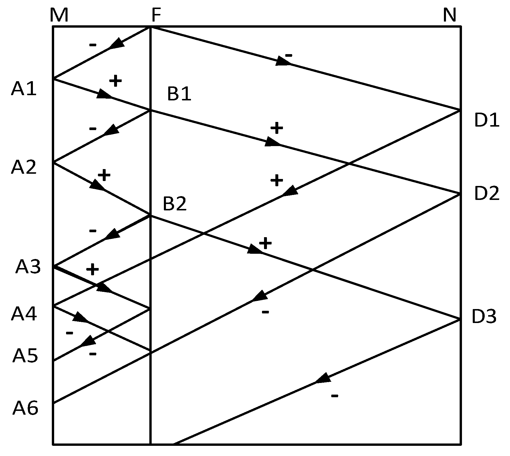
3. Traveling Wave Transmission Characteristics

When a short-circuit fault occurs somewhere in the cable, the magnetic field energy and electric field energy around the fault point are transformed into each other, and then voltage and current traveling waves are generated to the lines at both ends. According to the superposition principle, it can be equivalent to the normal component and the fault component voltage at the fault point. The additional voltage source generates fault voltage traveling waves with rich frequencies to both ends of the cable. When the fault voltage traveling wave propagates in the DC cable, its own refraction occurs at the fault point, and the polarity of the traveling wave will be changed by reflection instead of refraction. The grid is shown in Figure 2.
In the DC cable, the characteristic impedance (wave impedance) Z c m of each modulus and the modulus propagation coefficient γ m are calculated as follows [27]:
Z c m = Z m Y m = ( R m + j w L m ) ( G m + j w C m )
γ m = α m + j β m = Z m Y m = ( R m + j w L m ) ( G m + j w C m )
R m , G m , L m , C m are the modulus resistance, modulus conductance, modulus inductance, and modulus capacitance per unit length of the line, respectively.
Combining the above two formulas, we obtain:
α m = 1 2 [ ω 2 L m C m + R m G m + ( R m 2 + ω 2 L m 2 ) ( G m 2 + ω 2 C m 2 ) ] β m = 1 2 [ ω 2 L m C m R m G m + ( R m 2 + ω 2 L m 2 ) ( G m 2 + ω 2 C m 2 ) ]
In the formula, α m is the attenuation constant of each modulus, characterizing the attenuation characteristics of the traveling wave of each modulus; β m is the phase constant of each modulus, characterizing the phase change characteristics of the traveling wave of each modulus; w is the signal angular frequency; w = 2 f π .
Then, the formula for calculating the frequency-dependent wave velocity (propagation along the line) of each modulus of the DC cable is:
v m = w β m = 2 π f 1 2 [ w 2 L m C m R m G m + ( R m 2 + w 2 L m 2 ) ( G m 2 + w 2 C m 2 ) ]
The fault traveling wave signal can be decomposed into traveling wave components in different frequency segments. From Equations (9) and (10), it can be known that when different frequency components of traveling waves with different moduli propagate on the transmission line, the attenuation constant and propagation speed are different. This will cause traveling wave attenuation and dispersion, which will distort the traveling wave waveform. The higher the frequency of the traveling wave component, the more serious is the attenuation; that is, during the propagation process, the highest frequency component of the initial traveling wave head has the most serious attenuation. Under the attenuation of the initial wave head, the frequency band of the second traveling wave head will be reduced (the farther the distance is, the more the reduction will be); the speed of the traveling wave component and the singularity of the wave head will be weakened. The travel time of the component’s traveling wave to the measurement point increases. The detection of the second traveling wave head will directly cause errors in the ranging accuracy, and so using the double-ended traveling wave method to identify the first traveling wave head at both ends of the line will have a higher ranging accuracy.
If the total length of the line is L, it is assumed that, at the time t f , a short-circuit fault occurs at a distance d from the cable to the rectifier side, and the time when the initial traveling wave of the fault reaches the rectifier side and the inverter side is t M and t N , respectively. The propagation velocity of the voltage traveling wave in the cable is v; then the distance from the fault point to the rectifier terminal is shown in Equation (11).
d = ( L ( t N t M ) v ) 2
The relative positioning error is defined as Equation (12). Among them, Lm represents the measured fault distance, La represents the actual fault distance, and L0 represents the full length of the line.
ε = | L m L a L 0 | × 100 %
In this paper, the six-mode voltage is used as the ranging parameter; the propagation speed and attenuation constant of the six-mode voltage in the cable are comprehensively considered, and the fixed reference wave speed is selected as v = 1.978 × 10⁸ m/s.

4. The Principle of ILMD

4.1. The Principle of LMD

The local mean decomposition signal processing process [28] is as follows.
(1) For an original signal, determine all local extreme points in the signal, and calculate the average value of any two adjacent local extreme points and the estimated value of the amplitude envelope.
m i = ( n i + n i + 1 ) / 2
a i = | n i n i + 1 | / 2
(2) Connect the adjacent local mean points m i and m i + 1 and the amplitude envelope estimates a i and a i + 1 , and then smooth them with the moving average method to obtain the local mean function m 11 ( t ) and the amplitude envelope estimation function a 11 ( t ) , respectively. The calculation formula of moving average processing is as follows.
y s ( i ) = 1 2 n + 1 [ y ( i + n ) + y ( i + n 1 ) + + y ( i n ) ]
Among them, y ( i ) is the original sequence of data, and 2 n + 1 is the sliding width. When i < n , the span should be reduced accordingly, and the limit should not exceed the endpoint of the sequence.
(3) Separate the local mean function m 11 ( t ) from the original signal x ( t ) to obtain the signal h 11 ( t ) .
h 11 ( t ) = x ( t ) m 11 ( t )
(4) Divide h 11 ( t ) by the magnitude envelope estimation function a 11 ( t ) to obtain the FM signal s 11 ( t ) .
s 11 ( t ) = h 11 ( t ) a 11 ( t )
Repeat the above steps s 11 ( t ) . If the amplitude envelope estimation function a 12 ( t ) = 1 is obtained, this means that s 11 ( t ) is a pure FM signal. If a 12 ( t ) 1 , the above iterative process needs to be repeated until s 1 n ( t ) is a pure FM signal, as shown in the following formula.
{ h 11 ( t ) = x ( t ) m 11 ( t ) h 12 ( t ) = s 11 ( t ) m 12 ( t )   h 1 n ( t ) = s 1 ( n 1 ) ( t ) m 1 n ( t )
{ s 11 ( t ) = h 11 ( t ) a 11 ( t ) s 12 ( t ) = h 12 ( t ) a 12 ( t )   s 1 n ( t ) = h 1 n ( t ) a 1 n ( t )
The conditions for iterative termination are as shown in Equation (20). In practical applications, in order to avoid excessive decomposition times, an iteration termination threshold Δ is set. When 1 Δ a 1 n ( t ) 1 + Δ , the iteration terminates.
lim n a 1 n ( t ) = 1
(5) Multiply all the amplitude envelope estimation functions generated in the iterative process to obtain the instantaneous amplitude function a 1 ( t ) .
a 1 ( t ) = a 11 ( t ) a 12 ( t ) a 1 n ( t ) = k = 1 n a 1 k ( t )
(6) Multiply a 1 ( t ) and s 1 n ( t ) to obtain the first product function component of the original signal x(t).
P F 1 ( t ) = a 1 ( t ) s 1 n ( t )
(7) After separating the first product function component from the original signal x ( t ) , the remaining signal u 1 ( t ) is obtained, and the above steps are repeated with u 1 ( t ) as the new initial signal until u k ( t ) is a monotonic function. The calculation process is as follows.
{ u 1 ( t ) = x ( t ) P F 1 ( t ) u 2 ( t ) = u 1 ( t ) P F 2 ( t ) u k ( t ) = u k 1 ( t ) P F k ( t )
The final original signal can be reconstructed from u k ( t ) and all product function components.
x ( t ) = i = 1 k P F i ( t ) + u k ( t )

4.2. Hilbert Transform

Perform Hilbert transform on the product function components of the original signal x(t).
P F ¯ i ( t ) = 1 π + P F i ( τ ) t τ d τ
The corresponding analytical signal can be expressed by Equations (26) and (27).
Y i ( t ) = P F i ( t ) + j P F ¯ i ( t ) = a i ( t ) e j ϕ i ( t )
ϕ i ( t ) = arctan P F ¯ i ( t ) P F i ( t )
Derivation of the phase function gives the instantaneous frequency function.
f i ( t ) = 1 2 π ω i ( t ) = 1 2 π d [ arctan P F ¯ i ( t ) P F i ( t ) ] / d t
Figure 3 is the flowchart of the fault location of DC cables based on the improved LMD algorithm. The input fault signal is first decomposed by local mean value; the obtained amplitude envelope signal A is used as the final instantaneous amplitude function, and the PF1 component is used for Hilbert transform to obtain the instantaneous frequency function. The sudden change point of the instantaneous frequency curve is the moment when the wave head reaches the measurement end, and then the fault distance is calculated.

4.3. Comparison of Mathematical Methods

There is a significant difference in the solution methods for the local mean functions EMD and LMD. EMD uses cubic spline interpolation for all extreme points to obtain the upper envelope and lower envelope of the original signal and then uses the average method to obtain the local mean function. For LMD to solve the local mean function, the average of two adjacent extreme values is obtained, and the moving average algorithm is used to smooth it; we take a mathematical signal as an example and use LMD and EMD to decompose and then reconstruct. Observe Figure 4c and Figure 5b; compared with the original signal, the frequency and amplitude after EMD resynthesis are quite different, and the decomposition result of LMD is more accurate.
The LMD decomposition results are as follows:
Figure 4. Decomposition result of LMD. (a) Original signal. (b) PF component. (c) Comparison of the resynthesized signal with the original signal.
Processes 10 01655 g004
The EMD decomposition results are as follows:
Figure 5. Decomposition result of EMD. (a) IMF component. (b) Comparison of the resynthesized signal with the original signal.
Processes 10 01655 g005

5. Simulation Results

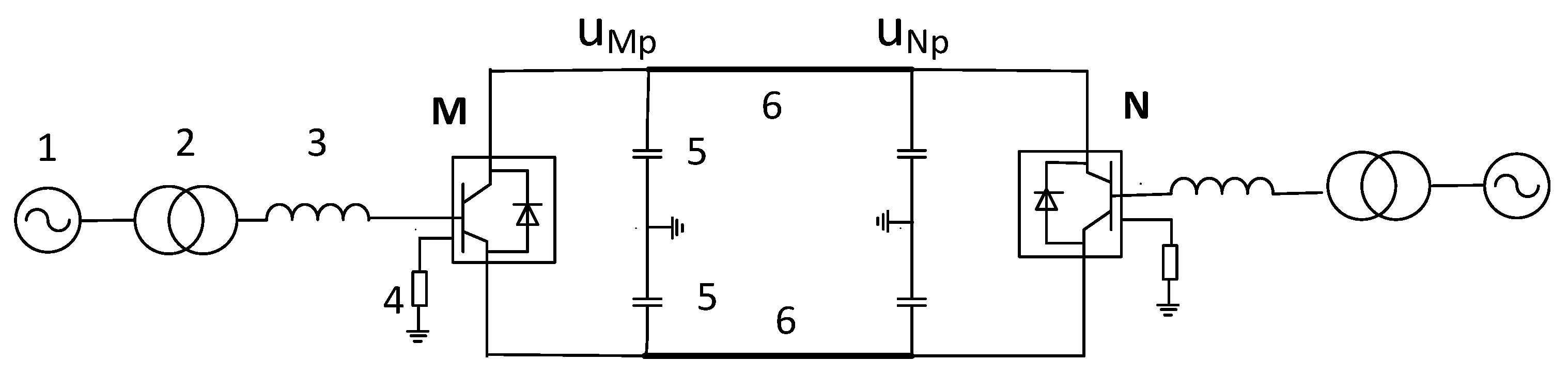
5.1. Power Transmission Model Construction

At present, there are three types of HVDC transmission model: distributed parameter model, equivalent thermal circuit model, and finite element model. When the wavelength of the electromagnetic wave is much smaller than the physical size of the corresponding network, it is necessary to use the distributed parameter model to characterize the power network, and so the distributed parameter model is more used in practical applications. The VSC-HVDC simulation system model established by PSCAD is shown in Figure 6. The AC system voltage is 50 Hz; the rated voltage is 220 kV; the rated DC voltage is ±320 kV; and the rated transmission power is 1000 MW. The three-phase fully controlled bridge circuit and the SPWM modulation control circuit are used. There is constant DC voltage and constant AC voltage control; the receiving end adopts constant active power and constant reactive power control; the rated DC voltage is set to 640 kV; the rated transmission active power is 1000 MW; and the reactive power is 0 Mvar. The single-core XLPE DC cable model adopts the armored frequency domain model, and the total cable length is 200 km.
Among them, ① represents the AC power supply; ② represents the converter transformer; ③ represents the converter reactor; ④ represents the AC filter; ⑤ represents the DC side capacitor; and ⑥ represents the DC cable.

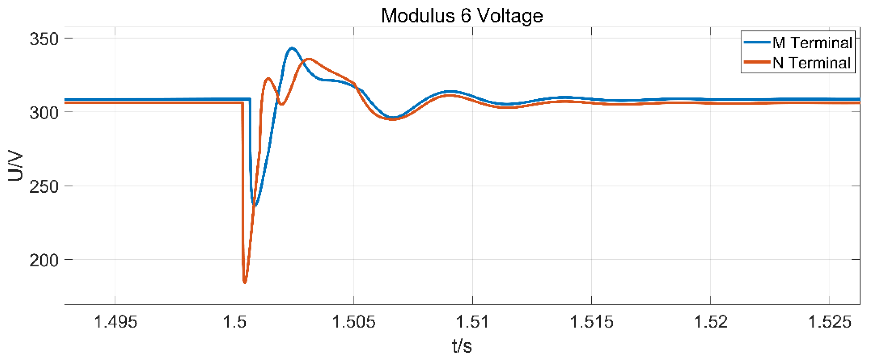
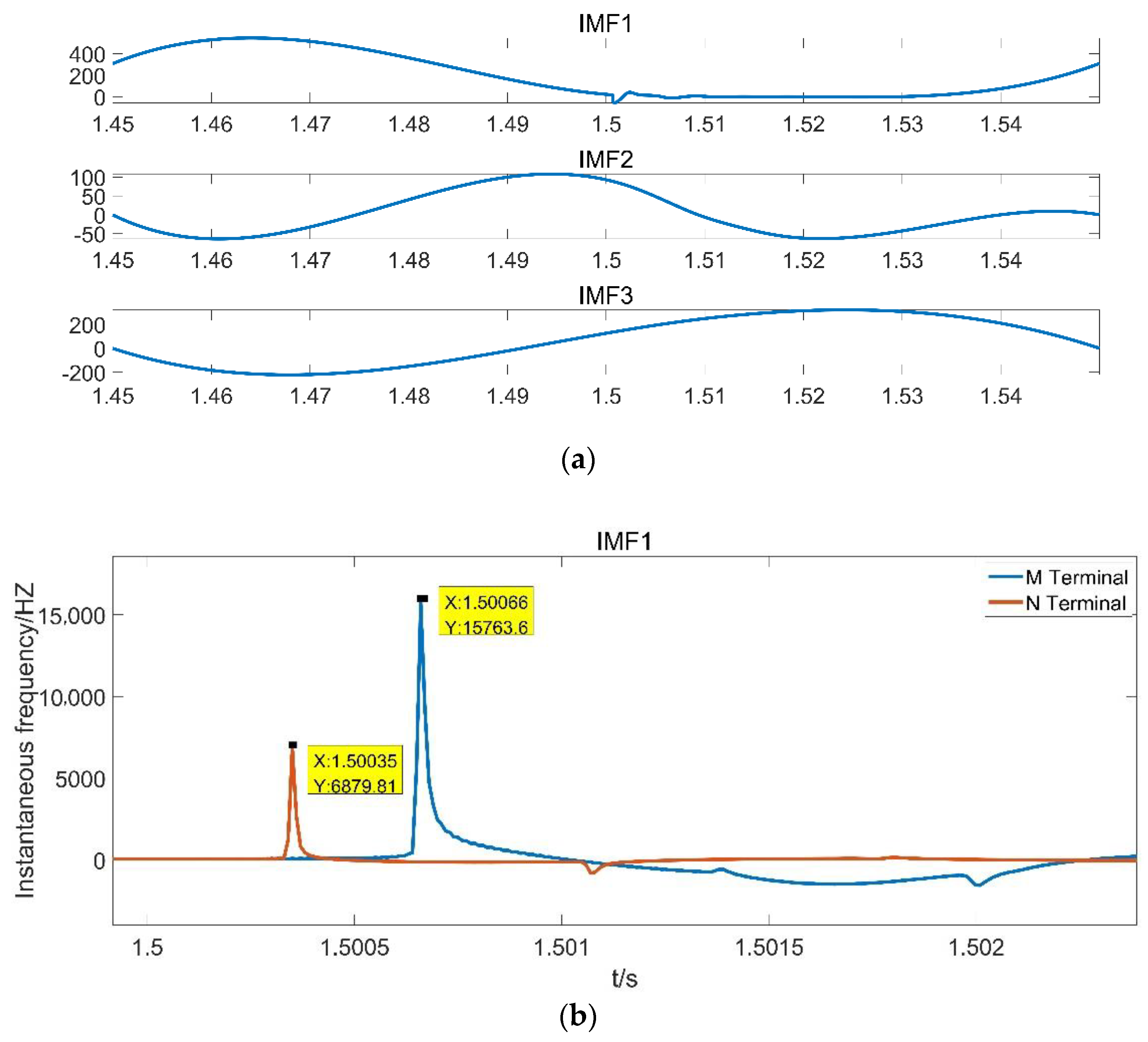
5.2. ILMD Method Validation

Using the above-mentioned building model, faults are set at different positions, and the improved LMD method is used for testing. Set the fault start time to 1.5 s, the fault duration to 0.02 s, and the sampling frequency to 0.1 MHz. Taking the metal ground fault 130 km away from the rectifier side as an example, take 1.45–1.55 s for data analysis. The corresponding fault current and fault voltage waveforms are shown in Figure 7, and the six-mode voltage waveform obtained by decoupling the rectifier side voltage is shown in Figure 8.
The six-mode voltage is decomposed by LMD to obtain the high-frequency component PF1 as shown in Figure 9a, and the Hilbert analysis is performed to obtain its instantaneous frequency function curve, as shown in Figure 9b. The frequency mutation points of the M-terminal and N-terminal correspond to the moments of 1.50065 s and 1.50035 s, respectively. Putting them into Equation (11), the theoretical value of the fault distance is 129.6699 km; the error distance is 0.33 km, and the error percentage is 0.165%.
The IMF component obtained by using HHT for the six-mode voltage component is shown in Figure 10a, and the instantaneous frequency of Hilbert transform of IMF1 is shown in Figure 10b. The frequency mutation points of the M-terminal and N-terminal appear at 1.50066 s and 1.50035 s, respectively. Putting them into Equation (11), the theoretical value of fault distance is 130.6590 km; the error distance is 0.659 km, and the error percentage is 0.3295%. Compared with HHT, ILMD has a high precision of 329 m, and, in the case of partial fault distance, the amplitude-frequency information, including the high-frequency feature quantity, is seriously polluted in the process of EMD decomposition, which makes it impossible to accurately locate.
In the fault location problem, the initial traveling wave front is the singular point, and the wavelet mode maxima can be used to identify the singular point. In the fault data in Figure 6, the wavelet modulus maxima are obtained by discrete stationary wavelet transform. The wavelet basis function and the number of decomposition layers are Daubechies (db4) and three layers, respectively, and the modulus maxima of the voltage at both ends are obtained as shown in Figure 11.
It can be seen from Figure 11 that the time when the initial traveling wave head reaches the M end and the N end corresponds to the 5069th and 5038th sampling points, respectively, and the corresponding time difference between the two sampling points is 0.00031 s. It can be calculated that the theoretical value of the fault distance is 130.6605 km; the error distance is 0.6605 km, and the relative error percentage is 0.3302%.
For metallic ground faults, the fault time is set to 1.5 s~1.52 s; the fault location is performed for different fault distance points; and the accuracy is compared with the methods using wavelet analysis and HHT. It can be obtained that the error of fault location using ILMD is significantly reduced compared with that of other methods. The corresponding experimental simulation data are shown in Table 1. Taking China as an example, according to the ‘National Electric Power Dispatching System “Tenth Five-Year” Science and Technology Development Plan Outline’ issued by State Grid, the comprehensive error should not exceed 1%. Due to technical and economic constraints, the ranging error cannot be too small. From a practical point of view, an absolute ranging error of less than 1 km can better meet the field requirements. The error in the ranging method proposed in this paper is up to more than 900 m under high impedance, and the error is smaller in most cases, which can meet the actual requirements of engineering.
The fault time is set as 1.5 s~1.52 s, and it is grounded through different transition resistances under different fault distances. The ILMD distance measurement results are shown in Table 2. It can be seen from Table 2 that, at the same fault point, the error only increases by a few meters in the case of high-impedance grounding; that is, the result of fault location is hardly affected by the transition resistance.

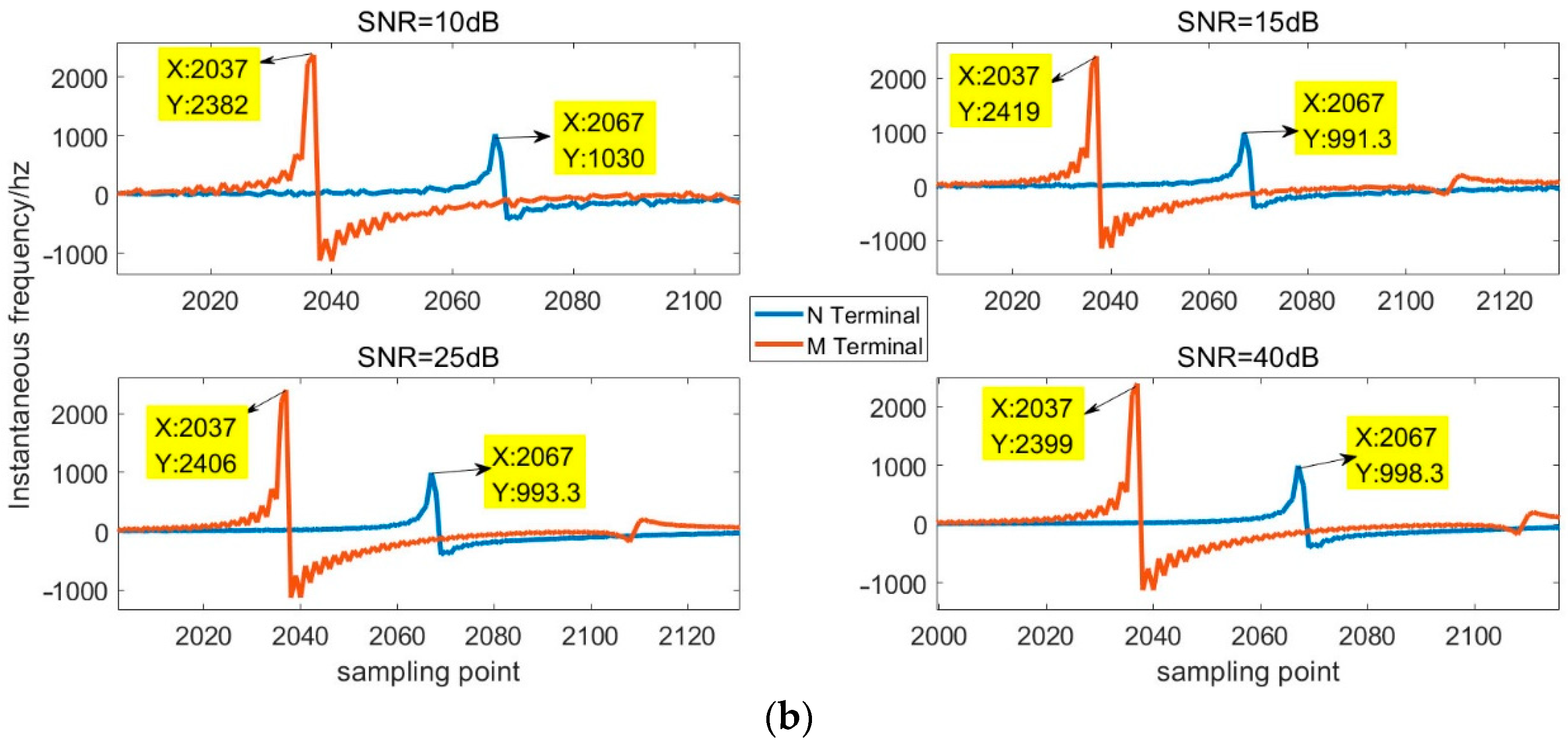
5.3. Noise Immunity Test

Cables generally use transformers to collect fault traveling wave signals, but the detection of transformers is susceptible to noise interference. The influencing factors and sources of noise can be divided into external factors and internal factors. External factors include line construction, electrical equipment interference, etc., while internal factors generally originate from random fluctuations within the transformer itself.
Take the metallic ground fault 130 km away from the rectifier side as an example, and add noise interference with a signal-to-noise ratio (SNR) of 20 dB to the voltage traveling wave signal, as shown in Figure 12a. Gaussian white noise with signal-to-noise ratios of 10 dB, 15 dB, 25 dB, and 40 dB is added to the fault signal, and the instantaneous frequency is obtained by ILMD analysis, as shown in Figure 12b. The 2037th and 2067th sampling points appear at the M-terminal and N-terminal frequency mutation points, respectively, corresponding to 1.50065 s and 1.50034 s. Putting them into formula (11), the theoretical value of the fault distance can be obtained as 129.6699 km, and the error is 0.3301 km. A large number of fault points are added with different proportions of noise for testing, and the results are shown in Table 3. When the signal-to-noise ratio (SNR) is less than 10 dB, the instantaneous frequency mutation point caused by the arrival of the wave head will be submerged, and accurate detection cannot be performed. When the signal-to-noise ratio SNR ≥ 15 dB, the ranging accuracy is high.

6. Conclusions

(1) This paper proposes a new fault location method for HVDC cable lines which combines LMD and Hilbert transform. It not only inherits the advantages of LMD in the decomposition process of the weak endpoint effect and of less pollution of amplitude-frequency information but also takes into account the ability of the Hilbert transform to completely retain the mutation information of the instantaneous frequency function. Through a large number of experimental verifications, the error of the proposed positioning method is within 1%; the positioning accuracy is high, and it is hardly affected by transition resistance and interference noise.
(2) Compared with HHT, the method in this paper has a small endpoint effect and less iteration processing, which avoids the large difference in the instantaneous frequency function extracted by HHT in some cases. Compared with wavelet transform, it overcomes the large positioning error in the case of high-resistance near-end faults, and the ranging accuracy meets the requirements of on-site operation and maintenance accuracy.

Author Contributions

W.C. proposed the initial idea and gave complete guidance and review to the logic of the whole article. Z.L. carried out the specific implementation of the plan and the article writing. M.X. participated in the construction of the transmission system model, and R.N. participated in the compilation of the parameters. All authors have read and agreed to the published version of the manuscript.

Funding

This work was supported in part by the Academic Degrees and Graduate Education Reform Project of Henan Province (No.2021SJGLX078Y), the Key Scientific Research Projects Plan of Henan Higher Education Institutions (No.19A470006), and the Cultivation Plan of Young Backbone Teachers in Colleges and Universities of Henan Province (No.2019GGJS104).

Institutional Review Board Statement

Not applicable.

Informed Consent Statement

Not applicable.

Data Availability Statement

The data that support the findings of this study are available from the corresponding author upon reasonable request.

Conflicts of Interest

The authors declare that the research was conducted in the absence of any commercial or financial relationships that could be construed as a potential conflict of interest.

References

  1. Song, Y.; Shi, W.; Huang, C.; Zhao, Y.; Yang, X. Research on the rationalization of field commissioning for multi-terminal HVDC projects-taking lugaozhao HVDC project for example. In Proceedings of the 2021 Annual Meeting of CSEE Study Committee of HVDC and Power Electronics (HVDC 2021), Beijing, China, 28–30 December 2021. [Google Scholar]
  2. Gomis-Bellmunt, O.; Sau-Bassols, J.; Prieto-Araujo, E.; Cheah-Mane, M. Flexible converters for meshed HVDC grids: From flexible AC transmission systems (FACTS) to flexible DC grids. IEEE Trans. Power Deliv. 2019, 35, 2–15. [Google Scholar] [CrossRef]
  3. Zhang, J.; Zhou, H.J.; Qian, J.F. A two-terminal fault location algorithm using asynchronous sampling based on genetic algorithm. In Proceedings of the 2011 International Conference on Advanced Power System Automation and Protection, Beijing, China, 16–20 October 2011; IEEE: Beijing, China, 2011; Volume 2, pp. 1513–1516. [Google Scholar]
  4. Gao, S.; Suonan, J.; Song, G.; Zhang, J.; Jiao, Z. Fault location method of DC transmission line based on distributed parameter model. Chin. J. Electr. Eng. 2010, 30, 75–80. [Google Scholar]
  5. Kang, L.; Tang, K.; Luo, J.; Xu, R.; Huang, J. Single-pole grounding double-ended fault location of DC transmission lines. Power Grid Technol. 2014, 38, 2268–2273. [Google Scholar] [CrossRef]
  6. Lu, D.; Liu, Y.; Xie, J.; Wang, B.; Liao, Q. Multi-Layer Model Enabled Fault Location for Underground Cables in MMC-HVDC Grids Considering Distributed and Frequency Dependent Line Parameters. IEEE Trans. Power Deliv. 2021, 37, 3082–3096. [Google Scholar] [CrossRef]
  7. Lin, S.; He, Z.; Li, X.; Qian, Q. A single-ended traveling wave natural frequency ranging method considering time domain characteristics. Power Grid Technol. 2012, 36, 243–248. [Google Scholar]
  8. Liao, K.; He, Z.; Li, X. Fault Location of HVDC Transmission Lines Based on Natural Frequency of Traveling Waves. Autom. Electr. Power Syst. 2013, 37, 104–109. [Google Scholar]
  9. He, Z.Y.; Liao, K.; Li, X.P.; Lin, S.; Yang, J.W.; Mai, R.K. Natural frequency-based line fault location in HVDC lines. IEEE Trans. Power Deliv. 2013, 29, 851–859. [Google Scholar] [CrossRef]
  10. He, J.; Li, B.; Sun, Q.; Li, Y.; Lyu, H.; Wang, W.; Xie, Z. The improved fault location method based on natural frequency in MMC-HVDC grid by combining FFT and MUSIC algorithms. Int. J. Electr. Power Energy Syst. 2022, 137, 107816. [Google Scholar] [CrossRef]
  11. Song, G.; Chu, X.; Cai, X.; Gao, S.; Ran, M. A fault-location method for VSC-HVDC transmission lines based on natural frequency of current. Int. J. Electr. Power Energy Syst. 2014, 63, 347–352. [Google Scholar] [CrossRef]
  12. Cao, W.; Chen, X.; Li, Z. Locating Natural Frequency Faults in HVDC Transmission Systems Based on the Rotation-Invariant Technology Signal Parameter Estimation Algorithm and the Total Least Squares Method. Math. Probl. Eng. 2022, 2022, 1467857. [Google Scholar] [CrossRef]
  13. Huang, Z. A new method for fault location of hybrid lines using natural frequencies of traveling waves. J. Electr. Power Syst. Autom. 2015, 27, 73–79. [Google Scholar]
  14. Liang, J.; Jing, T.; Niu, H.; Wang, J. Two-terminal fault location method of distribution network based on adaptive convolution neural network. IEEE Access 2020, 8, 54035–54043. [Google Scholar] [CrossRef]
  15. Ye, X.; Lan, S.; Xiao, S.J.; Yuan, Y. Single Pole-to-Ground Fault Location Method for MMC-HVDC System Using Wavelet Decomposition and DBN. IEEJ Trans. Electr. Electron. Eng. 2021, 16, 238–247. [Google Scholar] [CrossRef]
  16. Cui, H.; Tu, N. HVDC transmission line fault localization base on RBF neural network with wavelet packet decomposition. In Proceedings of the 2015 12th International Conference on Service Systems and Service Management (ICSSSM), Guangzhou, China, 22–24 June 2015; pp. 1–4. [Google Scholar] [CrossRef]
  17. Zhang, M.; Wang, H. Fault location for MMC–MTDC transmission lines based on least squares-support vector regression. J. Eng. 2019, 2019, 2125–2130. [Google Scholar] [CrossRef]
  18. Lan, S.; Chen, M.J.; Chen, D.Y. A novel HVDC double-terminal non-synchronous fault location method based on convolutional neural network. IEEE Trans. Power Deliv. 2019, 34, 848–857. [Google Scholar] [CrossRef]
  19. Zhang, C.; Song, G.; Wang, T.; Yang, L. Single-ended traveling wave fault location method in DC transmission line based on wave front information. IEEE Trans. Power Deliv. 2019, 34, 2028–2038. [Google Scholar] [CrossRef]
  20. Zhang, S.; Zou, G.; Huang, Q.; Gao, H. A traveling-wave-based fault location scheme for MMC-based multi-terminal DC grids. Energies 2018, 11, 401. [Google Scholar] [CrossRef] [Green Version]
  21. Xi, C.; Chen, Q.; Wang, L. A single-terminal traveling wave fault location method for VSC-HVDC transmission lines based on S-transform. In Proceedings of the 2016 IEEE PES Asia-Pacific Power and Energy Engineering Conference (APPEEC), Xi’an, China, 25–28 October 2016; IEEE: Xi’an, China, 2016; pp. 1008–1012. [Google Scholar]
  22. Zhang, M.; Guo, R.; Sun, H. Fault Location of MMC-HVDC DC Transmission Line Based on Improved VMD and S Transform. In Proceedings of the 2020 4th International Conference on HVDC (HVDC), Xi’an, China, 6–9 November 2020; IEEE: Xi’an, China, 2020; pp. 792–796. [Google Scholar]
  23. Li, Y.; Zhao, Y.; Kong, J.; Zhou, J.; Zheng, T. A Travelling Wave based Single-Ended Fault Location Using Multi-resolution Morphological Gradient. In Proceedings of the 2021 6th International Conference on Power and Renewable Energy (ICPRE), Shanghai, China, 17–20 September 2021; pp. 221–226. [Google Scholar] [CrossRef]
  24. Wang, D.; Hou, M. Travelling wave fault location algorithm for LCC-MMC-MTDC hybrid transmission system based on Hilbert-Huang transform. Int. J. Electr. Power Energy Syst. 2020, 121, 106125. [Google Scholar] [CrossRef]
  25. Yu, J.; Lv, J. Weak fault feature extraction of rolling bearings using local mean decomposition-based multilayer hybrid denoising. IEEE Trans. Instrum. Meas. 2017, 66, 3148–3159. [Google Scholar] [CrossRef]
  26. Zhao, P.; Chen, Q.; Sun, K.; Xi, C. A current frequency component-based fault-location method for voltage-source converter-based high-voltage direct current (VSC-HVDC) cables using the S transform. Energies 2017, 10, 1115. [Google Scholar] [CrossRef] [Green Version]
  27. Xi, C. Research on Fault Location of Flexible HVDC Transmission Lines; Shandong University: Shandong, China, 2017. [Google Scholar]
  28. Song, H.; Huang, C.; Liu, H.; Chen, T.; Li, J.; Luo, Y. A New Method for Detection of Power Quality Disturbance Based on Improved LMD. Chin. J. Electr. Eng. 2014, 34, 1700–1708. [Google Scholar] [CrossRef]
Figure 1. Equivalent circuit of bipolar cable.
Processes 10 01655 g001
Figure 2. Fault voltage traveling wave grid diagram.
Processes 10 01655 g002
Figure 3. Ranging flowchart.
Processes 10 01655 g003
Figure 6. Schematic diagram of VSC-HVDC DC transmission system.
Processes 10 01655 g006
Figure 7. Fault voltage and fault current.
Processes 10 01655 g007
Figure 8. Six-mode voltage fault waveform.
Processes 10 01655 g008
Figure 9. Analysis of faults at 130 km using ILMD. (a) PF1 component of six-mode voltage. (b) Instantaneous frequency curve.
Processes 10 01655 g009
Figure 10. Using HHT to analyze faults at 130 km. (a) IMF component. (b) Instantaneous frequency curve.
Processes 10 01655 g010
Figure 11. M-terminal and N-terminal voltage modulo maximum values.
Processes 10 01655 g011
Figure 12. Analysis of noisy signals. (a) Voltage traveling wave signal plus noise waveform. (b) Instantaneous frequency at different signal-to-noise ratios.
Processes 10 01655 g012aProcesses 10 01655 g012b
Table 1. Comparison of ILMD and other ranging methods.
Fault Distance (km)Wavelet Transform (km)Error
(%)
HHT
(km)
Error
(%)
ILMD
(km)
Error
(%)
01.05360.52680.98860.49430.77420.3871
108.01830.9909Error-9.01190.4940
5049.55840.220849.33500.332549.93500.0325
8584.17600.4120Error-85.16420.0821
100100.01250.00631000.00631000
130130.66050.3303130.65900.3295129.66990.1650
150150.54150.2708150.63920.3196150.43900.2195
180182.09101.0455182.08701.0435180.73910.3695
200198.67500.6625201.37620.6881198.96530.5173
Table 2. Algorithm ranging accuracy verification under different transition impedances.
Fault Distance (km)Transition Impedance
(Ω)
ILMD
(km)
Error
(%)
1009.01190.4940
1008.02290.9885
10008.02290.9885
20008.02290.9885
50049.93500.0325
10049.93500.0325
100049.93500.0325
200049.66090.1695
85085.16420.0821
10085.16580.0829
100085.16580.0829
200085.16500.0825
1300129.66990.1650
100130.65900.3295
1000130.65900.3295
2000130.65900.3295
1800180.73910.3695
100180.73910.3695
1000180.73910.3695
2000181.0980181.0980
Table 3. Algorithm ranging accuracy verification under different proportions of noise.
Fault Distance (km)SNR
(dB)
Ranging Results (km)Error
(%)
1040/25/159.01190.4940
5040/25/1549.93500.0325
8540/25/1585.16420.0821
10040/25/151000
13040/25/15129.66990.1650
18040/25/15180.73910.3695
Publisher’s Note: MDPI stays neutral with regard to jurisdictional claims in published maps and institutional affiliations.

