Article

Multi-Objective Optimal Scheduling for Multi-Renewable Energy Power System Considering Flexibility Constraints

1
State Key Laboratory of Power Transmission Equipment and System Security and New Technology, Chongqing University, Chongqing 400044, China
2
Electric Power Dispatching and Control Center of Yunnan Power Grid Co., Ltd., Kunming 650200, China
3
Electric Power Research Institute of Yunnan Power Grid Co., Ltd., Kunming 650217, China
*
Author to whom correspondence should be addressed.
Processes 2022, 10(7), 1401; https://doi.org/10.3390/pr10071401
Submission received: 28 June 2022 / Revised: 13 July 2022 / Accepted: 15 July 2022 / Published: 18 July 2022
(This article belongs to the Special Issue Modeling, Analysis and Control Processes of New Energy Power Systems)

Abstract

:
As renewable energy penetration increases, the lack of flexibility in a multi-renewable power system can seriously affect its own economics and reliability. To address this issue, three objectives are considered in this study: power fluctuations on tie-line, operating cost, and curtailment rate of renewable energy. Presented also is an optimal day-ahead scheduling model based on the MREPS for distributed generations with flexibility constraints. The multi-objective particle swarm optimization (MOPSO) algorithm can be applied to obtain a set of Pareto non-dominated solutions for the day-ahead scheduling strategy with the proposed model. By using fuzzy comprehensive evaluation, the optimal compromise solution is determined in the set. The presented method sacrifices a small amount of economy and power fluctuation, but it can reduce the deviation between forecast and realized power fluctuations on the tie-line, while improving the utilization of renewable energy.

1. Introduction

In modern power systems, the scarcity of fossil fuels and increasing pollution of the environment contribute to the development of renewable energy sources, such as solar and wind. Despite this, the stochastic nature of renewable energy generation is likely to have significant effects on system reliability and economy [1,2,3].
When operating a multi-renewable energy power system (MREPS), it is necessary to develop an optimal schedule to cope with the stochasticity of renewable energy generation [4,5]. MREPS scheduling is divided into two categories: day-ahead and real-time scheduling. There are several strategies for achieving various operational objectives using day-ahead scheduling. Reference [6] used a two-stage stochastic optimization model for an MREPS for minimizing the short-term operation cost, which introduces uncertainty in renewable generation, and showed that stochastic scheduling can provide significant reliability benefits to multi-energy supply systems. Reference [7] presented a day-ahead scheduling model that considers the seasonal uncertainty of renewable energy for a microgrid equipped with multi-renewable energy units. An improved optimization algorithm was proposed to solve optimization problems that focus on minimizing the operation cost. The results indicate that day-ahead scheduling based on the proposed algorithm can provide an efficient solution for managing MREPS energy. An MREPS is highly influenced by both economic indicators and the rate at which renewable energy is utilized, as illustrated in [8,9,10]. Furthermore, power fluctuations on the tie-line serve as relevant indicators for the main grid connected to an MREPS [11,12]. In the current MREPS scheduling process, the impact of these power fluctuations on the main grid is rarely considered. Although operating costs, curtailment rates of renewable energy, and power fluctuations on the tie-lines are all commonly considered in current studies on optimal dispatch [4,5,6,7,8,9,10,11,12,13,14,15], few studies consider these three indicators simultaneously. This can lead to a situation where, while some of these indicators are optimal, the other indicators may be poor. As a result, the present study proposes a day-ahead scheduling strategy based on operating costs, curtailment rates of renewable energy, and power fluctuations on the tie-lines.
In the case of real-time scheduling, the schedule is amended if the actual renewable energy output differs from the forecasted output. An improved particle swarm-optimization (PSO)-based strategy for managing energy over a two-time scale was presented in [16]. In day-ahead scheduling, one of the primary objectives is to achieve the most cost-effective schedule, and in real-time scheduling, the primary goal is to track day-ahead scheduling, compensate for power fluctuations, and maintain system stability. According to the experimental results, the proposed method could minimize the cost of generated electricity and maximize the efficiency of renewable energy systems. Real-time scheduling, however, relies on day-ahead scheduling. It is possible to increase the utilization rate of renewable energy if uncertainties associated with the generation of renewable energy can be properly incorporated into day-ahead scheduling. To address uncertainties in power systems [17,18,19], flexibility has been proposed. In [20], an optimal scheduling model for flexible resources was presented from both the generation and load sides. According to the results, a dynamic line rating model that incorporates optimal scheduling can maximize the utilization of flexible resources without curtailing wind power and minimize dispatch costs. Consequently, we propose a day-ahead scheduling strategy for an MREPS that accounts for flexibility constraints and concentrates on operation costs, renewable energy curtailment rates, and power fluctuations on the tie-line.
In this study, we attempt to solve a multi-objective optimization problem. It is possible to solve a multi-objective optimization problem in several ways. Among them, the linear weighted sum method and intelligent algorithms are frequently adopted. The linear weighted sum method is simple and fast, but it usually gives unclear physical results. In addition, the resulting error is typically large because several targets are of different dimensions and orders of magnitude. These factors remarkably impact the results and conclusions of practical problems [21]. Intelligent algorithms, which have clearer physical meaning, outperform the linear weighted sum method in accuracy, flexibility, and effectiveness in solving multi-objective problems. A number of intelligent algorithms have been successfully applied to engineering optimization, such as multi-objective particle swarm optimization (MOPSO) due to its unique search mechanism, excellent convergence performance, and convenient calculation capabilities [22,23]. As a result, MOPSO is adopted in this study to identify the Pareto non-dominated set of objective functions. Following the determination of the Pareto non-dominated solution set, a fuzzy comprehensive evaluation method [24] is adopted to determine the optimal compromise solution. The optimal day-ahead scheduling strategy can be determined based on the optimum compromise solution.
The contributions of this paper are summarized as follows:
1
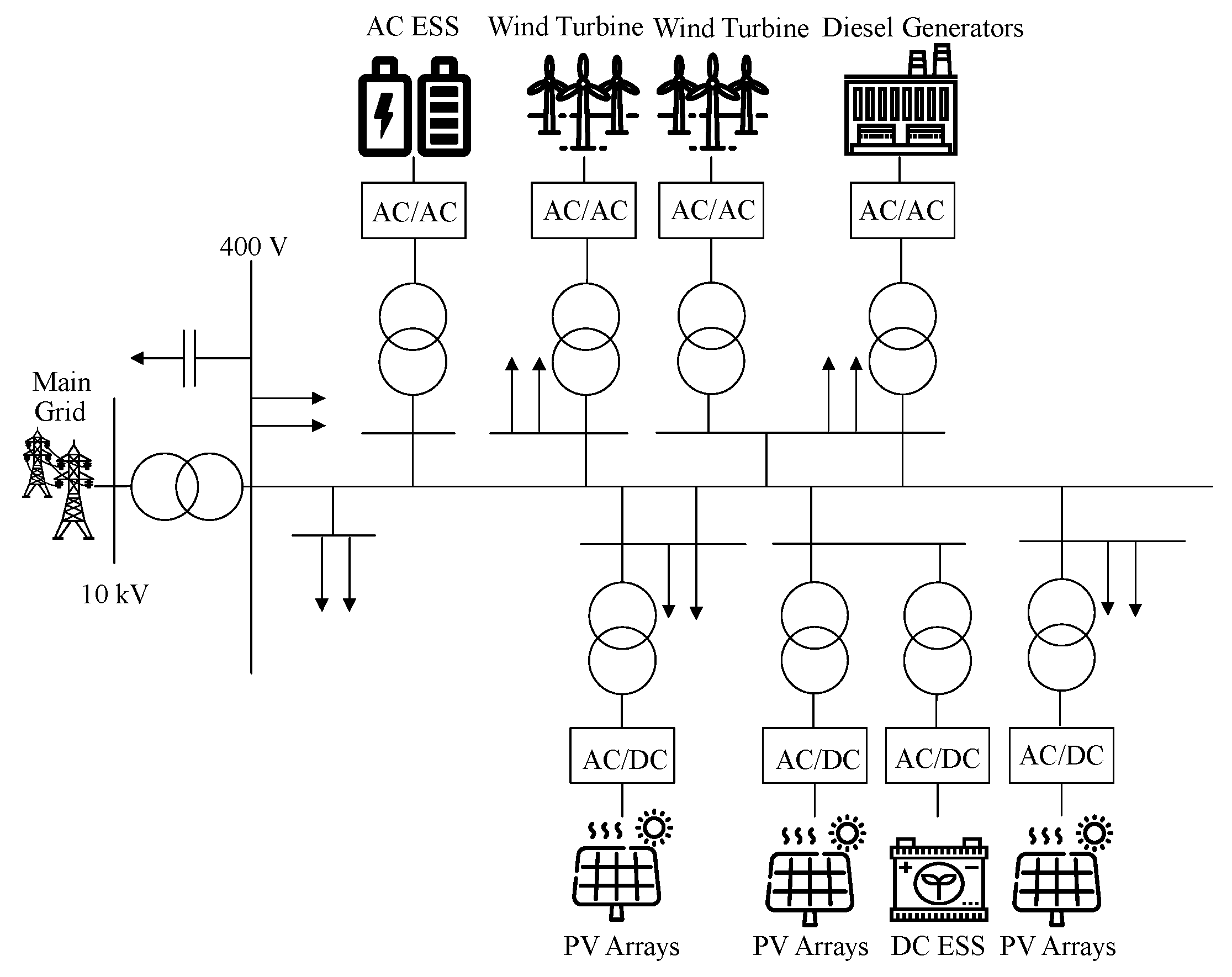
Considering the operation cost, renewable energy curtailment rates, and power fluctuations on the tie-line, a day-ahead scheduling model for the MREPS is established.
2
MOPSO and a fuzzy comprehensive evaluation method are used to evaluate the day-ahead scheduling model, and a day-ahead scheduling strategy for the MREPS considering flexibility is proposed.
Following is the remainder of this paper. The MREPS presents the day-ahead optimal scheduling model in Section 2, along with its constraints, taking flexibility into account. In Section 3, MOPSO and fuzzy comprehensive evaluation are discussed. An analysis of the experimental results is presented in Section 4, which simulates an actual MREPS. In Section 5, the conclusions are summarized.

2. Model for Multi-Objective Optimal Scheduling

The MREPS, consisting of wind turbines (WTs), photovoltaic (PV) arrays, diesel generators (DGs), energy storage systems (ESSs), and loads, only purchases electricity from the main grid. Figure 1 illustrates the details of the MREPS.

2.1. Objective Function

2.1.1. Operation Cost

A major consideration in the MREPS’s day-ahead scheduling is the operation cost. The operation cost mainly includes fuel cost, operation and maintenance, pollutant control, and purchased power cost. The daily operation cost of the MREPS can be expressed as follows:
F 1 = C fuel + C OM + C PC + C PP
where Cfuel, COM, and CPC are the total fuel, operation and maintenance (OM), and pollutant control (PC) costs associated with each distributed power generation in one day and CPP is the total cost of the purchased power (PP) from the main grid in one day. The formulas for Cfuel, COM, CPC, and CPP are as follows:
C fuel = n = 1 N t = 1 T ξ f . DG . n P DG . n ( t ) Δ t
C OM = m = 1 M t = 1 T ξ OM . m P m ( t ) Δ t
C PC = m = 1 M j = 1 J t = 1 T ξ m . j P m ( t ) Δ t
C PP = t = 1 T ξ PP ( t ) P PP ( t ) Δ t
where N is the total number of DGs; T is the total scheduling time; ξf.DG.n is the consumption cost per kW·h of the nth DG; PDG.n(t) is the output power of the nth DG in period t; Δt is the scheduling interval; M is the total number of distributed generation types; ξOM.m is the cost of operation and maintenance per kW·h of the mth type of distributed generation variety; Pm(t) is the output power of the mth type of distributed generation during period t; J is the total number of pollutant types; ξm.j is the emission cost factor for the jth type of pollutants generated by the mth type of distributed power generation; ξPP(t) and PPP(t) are the power purchased by the MREPS from the main grid for the period t, respectively.

2.1.2. Renewable Energy Curtailment Rate

The renewable energy curtailment rate is the ratio of the power curtailed by all renewable energy units to the total power that can be generated by renewable energy units during the dispatching period. The lower the value, the higher the utilization rate of renewable energy is. Utilization of the renewable energy is ideally increased while reducing the operation cost of the MREPS [15]. Thus, this study considers the curtailment rate of renewable energy. Following is the daily curtailment rate of the MREPS’s renewable energy:
F 2 = t = 1 T h = 1 H P h . c ( t ) / t = 1 T h = 1 H P h . all ( t )
where H represents the total number of the renewable energy types; Ph.c(t) and Ph.all(t) reflect the power curtailment and the available power generation of the hth type of renewable energy in period t, respectively.

2.1.3. Tie-Line Power Fluctuations

The frequent power exchange between the MREPS and the main grid can be attributed to the stochastic nature of renewable energy. In general, the unit commitment and economic load dispatch of the main grid have no impact on the MREPS. This is because the MREPS can be self-sufficient. Only when the MREPS is not self-sufficient, it is necessary for the main grid to help the MREPS to achieve power balance through unit commitment or economic load dispatch. As a consequence, the significant fluctuation in power on the tie-line has a negative impact on the main grid. The MREPS day-ahead scheduling must be designed to take into account power fluctuations across the tie-line.
As the square root of the variance, the standard deviation is a metric used to measure how dispersed a dataset is relative to its mean. Consequently, the standard deviation is typically used to describe the fluctuation of a data series. However, the standard deviation lacks comparability for different objects or samples with varying means of the same object. Hence, the coefficient of variation is used in this study to avoid these problems.
As a measure of data dispersion around the mean, the coefficient of variation represents the ratio of the standard deviation to the mean for a series of data points. The degree of variation from one data series to another can be compared, although the means are remarkably different from one another. A small variation indicates a small fluctuation degree [11]. On the tie-line, the power fluctuation can be defined as follows:
F 3 = 1 T t = 1 T ( P TL ( t ) μ TL ) 2 / μ TL
where PTL(t) represents the transmission power of the tie-line during period t and μTL represents the average transmission power of the tie-line during one day, which can be expressed as follows:
μ TL = 1 T t = 1 T P TL ( t )
Based on the above three objectives, the total objective function for the multi-objective optimal scheduling model is as follows:
min F = [ F 1 , F 2 , F 3 ]

2.2. Constraint Conditions

2.2.1. Constraints on the Power Balance

During the operation of the MREPS, at the end of each period, the sum of the output power of the DGs, the charging and discharging power of the ESS, and the purchased power from the main grid should be equal to the net load (NL) power of the system. As a result of this relationship, we may state:
P DG ( t ) + P ESS ( t ) + P TL ( t ) = P L ( t ) P WT ( t ) P PV ( t ) = P NL ( t )
where PDG(t) is the sum of the output power of the DGs in period t; PESS(t) is the charge and discharge power of the ESS in period t and becomes negative when the ESS is being charged; PTL(t) is the transmission power of the tie-line in period t; PL(t), PWT(t), PPV(t), and PNL(t) are the load power, output of WTs, output of PV arrays, and net load power in period t, respectively.

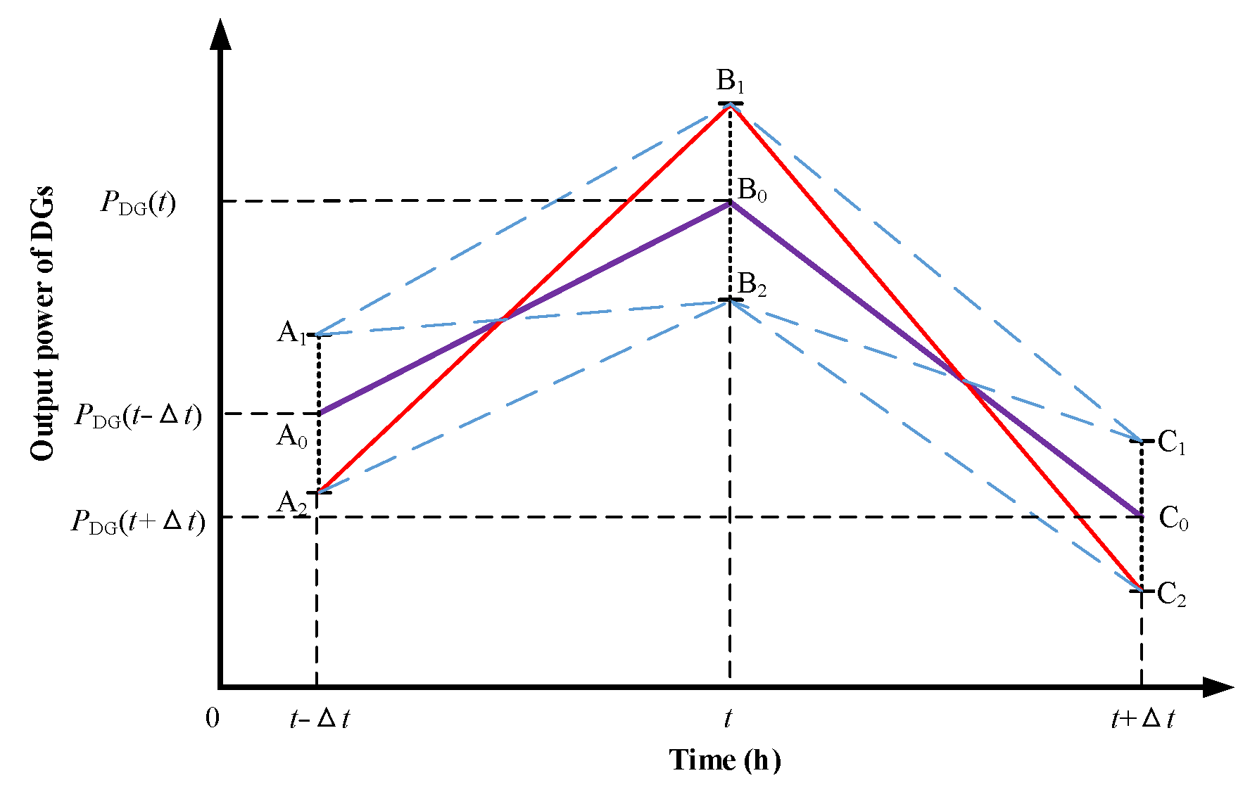
2.2.2. Constraints of Output Power for DGs Considering Flexibility

In light of the uncertainty associated with renewable energy generation, it is imperative that the MREPS be flexible. The DG is a commonly used flexible resource in MREPSs because of its satisfactory controllability and fast response speed. Therefore, flexibility should be considered and exploited in the output power constraints of DGs.
The uncertainty of renewable energy generation leads to prediction errors in net load power and the MREPS’s flexibility requirements. These flexibility requirements are provided by DGs in the MREPS. DGs are typically restricted in their output power range as follows [7]:
P DG ( t ) P DG . min P DG ( t ) P DG . max
where PDG.min and PDG.max represent the minimum and maximum output power of DGs, respectively.
In terms of conventional constraints, DGs are only considered for their minimum and maximum output. Due to these constraints, the output power of DGs may be inflexible during operation. When large prediction errors occur, DGs output power fails to meet the flexibility requirements. Therefore, new constraints that consider flexibility based on conventional constraints can be expressed as follows:
P DG ( t ) ( P DG . min + F NL . D ( t ) ) P DG ( t ) ( P DG . max F NL . U ( t ) )
where FNL.U(t) and FNL.D(t) represent the maximum upward and downward flexibility requirements of the MREPS in each period t.
Because of the error in predicting net load power, the MREPS is required to be flexible. Variables such as wind, solar, and load power are among the factors that affect the prediction errors of the net load power. As a result, wind, solar, and load power prediction errors are assumed to follow a normal distribution with a zero mean [25]. σPV(t), σWT(t), and σL(t) have the following standard deviations:
σ PV ( t ) = 0.2 W PV . F ( t ) + 0.02 W PV . C σ WT ( t ) = 0.2 W WT . F ( t ) + 0.02 W WT . C σ L ( t ) = 0.02 W L . F ( t )
where WPV.F(t), WWT.F(t), and WL.F(t) are the predicted wind, solar, and load power in period t, respectively, and WPV.C and WWT.C are the total installed capacity of PV arrays and WTs, respectively.
There are no correlations among wind, solar, and load power prediction errors. According to the basic characteristics of the normal distribution, the sum of two independent normally distributed random variables is normal, with the sum of the two means as the mean and the sum of the two variances as the variance. Hence, prediction errors of the net load power also follow the normal distribution with mean zero and standard deviation σNL(t), as shown below:
σ NL ( t ) = σ PV 2 ( t ) + σ WT 2 ( t ) + σ L 2 ( t )
The MREPS must offer flexibility equal to the forecast errors of net load power. However, in the prediction of net load power, there is a very small probability of maximum errors. Hence, the scenario where the flexibility requirement and forecast error are equal is uneconomical and wasteful. As a result, we need to consider the confidence intervals of these prediction errors. If the confidence level is 1 − α, then FNL.U(t) and FNL.D(t) can be expressed as:
F NL . U ( t ) = u 1 α / 2 σ NL ( t ) F NL . D ( t ) = u 1 α / 2 σ NL ( t )
where u1−α/2 is the upper (1 − α/2) critical value for the standard normal distribution.
Conventional ramping-rate constraints of DGs are expressed as follows:
P DG ( t ) P DG ( t Δ t ) R DG . max D Δ t P DG ( t ) P DG ( t Δ t ) R DG . max U Δ t
where R DG . max D and R DG . max U are the maximum downward and upward ramping rates of DGs, respectively, with both values positive, and Δt is the time interval.
Conventional constraints only consider the minimum and maximum ramping rates. The maximum ramping rate of DGs may occur in some periods under these constraints. The output power of DGs fails to meet the fluctuation of the net load power in this situation when DGs lack the ramping rate. Consequently, ramping-rate constraints should take flexibility into consideration.
As shown in Figure 2, A0, B0, and C0 are the prediction output power values of DGs at different times. DGs must reduce their output power to A2 if the maximum downward prediction errors of the net load power occur at time t − Δt. According to Equation (15), the reduced output power should be equal to FNL.D(t − Δt). It is imperative that the DGs increase their output power to B1 if they experience maximum upward prediction errors at time t. According to Equation (15), the increased output power should be equal to FNL.U(t). Therefore, the margin of the ramping rate that DGs should reserve is the sum of FNL.D(t − Δt) and FNL.U(t) from time t − Δt to time t. Similarly, the margin of the ramping rate that DGs should reserve is the sum of FNL.U(t) and FNL.D(t + Δt) from time t to time t + Δt. As a result, new constraints that consider flexibility can be expressed as follows:
P DG ( t ) P DG ( t Δ t ) R DG . max D Δ t + ( F NL . D ( t ) + F NL . U ( t Δ t ) ) P DG ( t ) P DG ( t Δ t ) R DG . max U Δ t ( F NL . U ( t ) + F NL . D ( t Δ t ) )

2.2.3. Constraints of the ESS Considering Flexibility in Charging and Discharging

In this study, the main function of the ESS is to provide assistance to DGs and ensure that DGs have adequate flexibility. Thus, the ESS and its conventional constraints are similar in terms of charging and discharging power:
S ESS ( t + Δ t ) = ( 1 δ ) S ESS ( t ) Δ t α ESS ( t ) P ESS ( t ) E ESS S ESS . min S ESS ( t ) S ESS . max P E S S ( t ) Δ t η ESS E ESS
where SESS(t) represents the state of charge (SOC) of the ESS in period t; δ represents the self-discharge efficiency of the ESS; EESS represents the maximum capacity of the ESS; SESS.min and SESS.max represent the minimum and maximum SOC of the ESS, respectively; Δt′ represents an hour; ηESS represents the percentage of the maximum charge–discharge capacity per hour to the maximum capacity of the ESS; αESS(t) represents the charge–discharge efficiency of the ESS in period t. The following formula can be used to calculate αESS(t):
α ESS ( t ) = α c , P ESS ( t ) < 0 1 / α d , P ESS ( t ) > 0
where αc and αd are the charge and discharge efficiencies of the ESS, respectively.
DGs, however, fail to achieve the maximum prediction error of the net load power. Because of this, we should take into account flexibility in the power constraints of the ESS when charging and discharging. This is because the secondary function of the ESS is to meet these maximum prediction errors. Here are the revised constraints:
S ESS ( t + Δ t ) = ( 1 δ ) S ESS ( t ) Δ t α ESS ( t ) P ESS ( t ) E ESS ( S ESS . min + F ESS . U ) S ESS ( t ) ( S ESS . max F ESS . D ) P E S S ( t ) Δ t η F . ESS E ESS
where FESS.U and FESS.D are the reserved SOC of the ESS and ηF.ESS is the percentage of the maximum charge–discharge capacity per hour to the maximum capacity of the ESS after considering flexibility.
If the maximum prediction error of the net load power occurs, DGs are capable of meeting most of these prediction errors. There is only a small portion of these prediction errors that must be met by the ESS. As a result, the constraints of FESS.U, FESS.D, and ηF.ESS are as follows:
0 F ESS . U 0.1 0 F ESS . D 0.1 0.8 η ESS η F . ESS η ESS
Since the ESS operation is periodic, the initial SOC should be equal to the final SOC in a day and expressed as follows:
S ESS ( t = 0 ) = S ESS ( t = T )
where T represents the total scheduling time.

2.2.4. Tie-Line Transmission Power Constraints in Consideration of Flexibility

In the MREPS, DGs and the ESS can sometimes fail. In this case, the tie-line must be flexible to facilitate the normal functioning of the MREPS. Therefore, the power limitation for tie-line transmission considering flexibility is expressed as follows:
P TL . min P TL ( t ) P TL . max F TL . U ( t )
where PTL.min and PTL.max represent the minimum and maximum transmission power of the tie line, respectively, and FTL.U(t) represents the reserved transmission power of the tie-line that can be increased in period t.
Load shedding is prohibited in the operation of the MREPS. In the event that DGs and the ESS fail, it is necessary to reserve the transmission power on the tie-line, which may be increased in case of a breakdown. However, if the load power decreases, then we may be able to achieve power balance by reducing the output power of DGs or curtailing the use of renewable energy sources. As a consequence, it is not necessary to reserve the transmission power of the tie-line.

3. Algorithm for the Solution of the Multiobjective Optimization Model
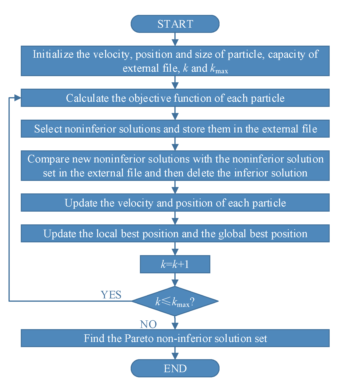
3.1. MOPSO

The multi-objective optimization problem in the presented model is solved via MOPSO in this study. Although MOPSO is one of the commonly used intelligent optimization algorithms [22,23], it is briefly introduced since it is the core of the algorithm in this paper. MOPSO updates the position and the velocity of each particle in every iteration and searches for the local and global best positions of particles. The velocity is modified and updated as follows:
v i k + 1 = ω v i k + c 1 r 1 ( p l k x i ) + c 2 r 2 ( p g k x i )
where v i k and xi are the velocity and position of the ith particle in the kth iteration; p l k is the local optimal position of the ith particle; p g k is the global optimal position of particles; ω is the inertia weight that influences the local and global exploitation abilities for MOPSO; c1 and c2 are the cognitive and social learning factors that maintain the movement of particles to the local and global optimal positions, respectively; r1 and r2 are two uniform random functions in the range [0,1].
Constraints of the velocity are expressed as follows:
v i k + 1 = v max ,             v i k + 1 > v max v i k + 1 = v min ,             v i k + 1 < v min
where vmin and vmax are the minimum and maximum velocities of particles, respectively.
The position of particles is indicated as follows:
x i k + 1 = x i k + v i k
MOPSO obtains the non-dominated solution set, unlike the single-objective PSO algorithm. Therefore, an external file is needed to store the set. The flowchart of MOPSO is shown in Figure 3.
The SOC of the ESS, the output power of DGs, and the tie-line transmission power are unknown in this study. Therefore, the SOC of the ESS and the output power of DGs in each period are considered decision variables. The tie-line power of transmission in each period can be obtained using Equation (10). Due to the fact that the set of Pareto non-dominated solutions is determined by these decision variables, each solution in the set corresponds to an operation state of the MREPS. Therefore, if we wish to determine the optimal day-ahead scheduling strategy, then we need to first identify the optimum compromise solution from the set of non-dominated Pareto solutions.

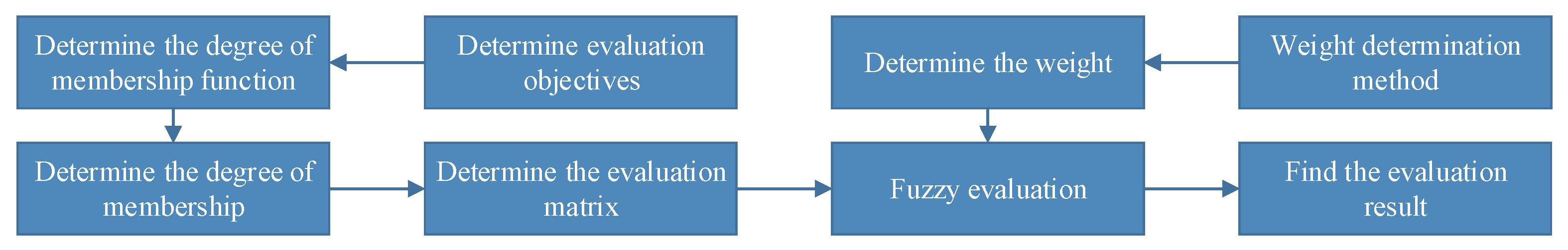
3.2. Fuzzy Comprehensive Analysis Methodology

This study employs the fuzzy comprehensive evaluation method to determine the most appropriate compromise solution. An effective and widely adopted method for evaluating hierarchical and integrated problems is a fuzzy comprehensive evaluation. The top two critical steps of this method are determining the weight vector of each evaluation objective appropriately and selecting the appropriate fuzzy membership function. Figure 4 illustrates the fuzzy comprehensive evaluation method flowchart.
Assume that X is the Pareto non-dominated solution set, which is expressed as follows:
X = x 11 x 1 j x 1 n x i 1 x i j x i n x m 1 x m j x m n
where m is the total number of objectives, n is the total number of the Pareto non-dominated solutions, and xij is the value of the ith objective of the jth Pareto non-dominated solution. To determine the most effective compromise solution from the Pareto non-dominated solution set, follow the steps outlined below:
(1)
For determining the membership degree of each objective in each Pareto non-dominated solution, a single-factor fuzzy evaluation is adopted. The fuzzy relation matrix can then be obtained as follows:
R = r 11 r 1 j r 1 n r i 1 r i j r i n r m 1 r m j r m n
where rij is the membership degree of the ith objective in the jth Pareto non-dominated solution. rij can be calculated as follows:
r i j = 1         ,     x i j X _ i X ¯ i x i j X ¯ i X _ i , X _ i < x i j < X ¯ i 0         ,     x i j X ¯ i
where X _ i and X ¯ i are the minimum and maximum expectations of the decision-maker for the ith objective, respectively.
(2)
The analytic hierarchy process (AHP)-entropy weight method (EWM) can be employed to determine the comprehensive weight vector for each objective. Assume that the comprehensive weight vector is:
A = [ ω 1 , ω 2 , , ω i , , ω m ] T
where ωi is the comprehensive weight vector of the ith objective. A can then be calculated using the following equation:
ω i = ω i ω i i = 1 m ( ω i ω i )
where ω i and ω i are the objective weights based on AHP and EWM, respectively. The discussion on AHP [26] and EWM [27] is excluded from this paper given that both have been extensively analyzed in the literature.
(3)
The comprehensive fuzzy evaluation vector B can be calculated as follows:
B = A R = [ b 1 , b 2 , , b j , , b m ] b j = i = 1 m ( ω i r i j )
where bj is the membership degree of the jth Pareto non-dominated solution.
When bj is close to 1, we can evaluate the jth Pareto non-dominated solution comprehensively. Therefore, from the set of Pareto non-dominated solutions, the optimal compromise solution corresponds to the maximum bj.

4. Case Study

Practical MREPS data are presented in this study within a simulation and analysis environment. The parameters of each power supply unit in the MREPS are listed in Table 1. The cost of each distributed generation is presented in Table 2. Table 3 presents the pollutant emission coefficients generated by each distributed generation. Table 4 shows the electricity purchase price of the MREPS from the main grid [15].
This study adopts a simulation of the load and output date of a typical day in the MREPS for WTs and PV arrays. To determine an optimal scheduling strategy, the forecast values of these data are used. Utilizing the realized values of these data, the optimal scheduling strategy is evaluated. Figure 5 and Figure 6 present the predicted and realized curves for the load and output from WTs and PV arrays in the MREPS for a typical day, respectively.
As shown in Section 4, it is possible to determine the optimal scheduling strategy of a typical day after obtaining the non-dominated solution set. On the basis of the models, constraints, data, and decision variables of this study, the non-dominated solution set of objectives can therefore be obtained using MOPSO. Figure 7 and Figure 8 illustrate non-dominated solutions based on the conventional and proposed strategies, respectively. From Figure 7 and Figure 8, we can see that the three objectives cannot reach the optimal solution at the same time for the non-dominated solution set obtained by MOPSO. The distribution of the non-dominated solution set shows a narrow shape at both ends and is wide in the middle.
Furthermore, Figure 7 and Figure 8 indicate that the non-dominated solution set of the proposed strategy is larger than that of the conventional strategy. According to this finding, after evaluating the flexibility constraints, the MREPS will sacrifice a portion of the economy, the utilization rate of renewable energy, and power fluctuations.
We must then determine the optimal compromise solution from the Pareto non-dominated solution set to find the optimal day-ahead scheduling strategy for a typical day. The fuzzy comprehensive evaluation method can be used to obtain optimal compromise solutions from non-dominated Pareto solution sets, based on the conventional and proposed strategies, as discussed in Section 4. By the fuzzy comprehensive evaluation method, Point A and Point B are the solutions with the highest evaluation scores in the respective non-dominated solution sets of Figure 7 and Figure 8, respectively. Therefore, Points A and B represent optimal compromise solutions in Figure 7 and Figure 8, respectively.
Finally, based on the relevant decision variables, the optimal day-ahead scheduling strategy for a typical day according to every optimal compromise solution can be determined. These are illustrated in Figure 9 and Figure 10.
Using the conventional and proposed strategies, Strategies A and B provide an optimal scheduling strategy for the typical day based on what has been denoted, respectively, for ease of use. Figure 9 and Figure 10 illustrate Strategy A’s preference for purchasing electricity from the main grid. It was found that the tie-line transmission power of Strategy A is close to its average. The consequence is a relatively low level of power fluctuations at the tie-line under Strategy A, whereas Strategy B prefers to generate electricity from DGs. It is more expensive to generate electricity through DGs than to purchase electricity from the main grid; therefore, Strategy B has a higher operation cost.
To better compare Strategies A and B, they were both applied in the context of a realistic scenario based on a typical day. Figure 5 shows such a situation. In Figure 11 and Figure 12, the realized operation results under Strategies A and B are presented, respectively.
The realized output of WTs and PV arrays is larger than the predicted value, as depicted in Figure 5 and Figure 6. Consequently, the realized output power of DGs in both Figure 11 and Figure 12 is smaller than the predicted value. However, DGs based on Strategy A generally have a minimum output power. DGs fail to reduce the output power in this case. Hence, curtailing renewable energy is the most economical way to maintain power balance after the ESS absorbs the excess power to the extent possible. By comparison, DGs based on this strategy are able to reduce the output power because Strategy B takes flexibility constraints into account. Therefore, the MREPS can decrease the output power of DGs to increase the utilization rate of renewable energy. In addition, Strategy B reduces the power purchased from the main grid during peak load periods from 18:00 to 22:00 in comparison to Strategy A. This phenomenon significantly eases the demand for power on the main grid during peak load periods.
The simulation results of Strategies A and B are listed in Table 5. It can be seen that Strategy A has a lower forecast operation cost, forecast curtailment rate of renewable energy, and forecast power fluctuations on the tie-line. All three indicators are higher for Strategy B. However, the IFR is 31.47% higher, the FSR is 45.83% lower, and the AIF is 13.36 kW/h higher for Strategy A compared to Strategy B. This indicates that Strategy A is less capable of coping with uncertainties during the real-time operation of the MREPS compared to Strategy B. This is corroborated by the real-time operation results of the two strategies.
What is more, the MREPS is operating at a higher cost under Strategy B, and the tie-line power fluctuations are 9.52% higher than they are under Strategy A. However, the rate of utilization of renewable energy for the MREPS under Strategy B is 18.03% higher than that under Strategy A. In addition, the deviation rate of forecast and realized power fluctuations of power under Strategy B is 14.59% lower than that under Strategy A. These findings indicate that Strategy B can reduce the deviation between forecast and realized power fluctuations on the tie-line and increase the utilization of renewable energy at the expense of a small amount of economy and power fluctuations at the same time. Moreover, the realized values of the three objectives under Strategy A increased by 16.79%, 37.58%, and 0.47% compared with their forecast values. In comparison with their forecast values, the realized values of the three objectives under Strategy B increased by 12.27%, 12.59%, and 0.05%. Based on this finding, the results formulated by Strategy B are more consistent with the realized operation results.

5. Conclusions

In this study, a day-ahead scheduling strategy designed to account for flexibility constraints was presented. A multi-objective problem was solved using MOPSO, and a set of the non-dominated solutions was derived for the three objectives. Using the fuzzy comprehensive evaluation method, the optimal compromise solution of the non-dominated solution set was determined. In addition, the optimal strategy proposed in this study was the day-ahead scheduling strategy corresponding to the optimal compromise solution. During peak load periods, the simulation results showed that the proposed strategy was effective in relieving the main grid’s pressure on power supply. Moreover, compared with those formulated using the conventional strategy, the results obtained from day-ahead scheduling formulated using the proposed strategy were closer to the results obtained from the MREPS. Although the economy and power fluctuations on the tie-line were slightly higher under the revised strategy, renewable energy usage was significantly higher, and the differences between forecast and realized power fluctuations on the tie-line were relatively small. This finding showed that the revised strategy has the potential to significantly improve the flexibility and reliability of the MREPS’s operation at the cost of a small amount of economy and fluctuations in power supply.

Author Contributions

Conceptualization, L.Y. (Lei Yang); and Q.W.; methodology, L.Y. (Lei Yang); software, C.G. and D.Z.; validation, W.H., C.X., and L.Y. (Longjie Yang). All authors have read and agreed to the published version of the manuscript.

Funding

This research received no external funding.

Institutional Review Board Statement

Not applicable.

Informed Consent Statement

Not applicable.

Data Availability Statement

The data presented in this study are available on request from the corresponding author. The data are not publicly available due to data confidentiality requirements.

Conflicts of Interest

The authors declare no conflict of interest.

References

  1. Hong, Z.; Hao, S.; Zhang, Q.; Kong, G. Microgrid Spinning Reserve Optimization with Improved Information Gap Decision Theory. Energies 2018, 11, 2347. [Google Scholar]
  2. Cz, A.; Hc, A.; Lu, L.; Zhang, H.; Zhang, X.; Li, G. Coordination planning of wind farm, energy storage and transmission network with high-penetration renewable energy. Int. J. Electr. Power Energy Syst. 2020, 120, 105944. [Google Scholar]
  3. Li, J.; Liu, J.; Yan, P.; Li, X.; Zhou, G.; Yu, D. Operation Optimization of Integrated Energy System under a Renewable Energy Dominated Future Scene Considering Both Independence and Benefit: A Review. Energies 2021, 14, 1103. [Google Scholar] [CrossRef]
  4. Menezes, R.; Soriano, G.D.; Aquino, R. Locational Marginal Pricing and Daily Operation Scheduling of a Hydro-Thermal-Wind-Photovoltaic Power System Using BESS to Reduce Wind Power Curtailment. Energies 2021, 14, 1441. [Google Scholar] [CrossRef]
  5. Wang, L.; Li, Q.; Ding, R.; Sun, M.; Wang, G. Integrated scheduling of energy supply and demand in microgrids under uncertainty: A robust multi-objective optimization approach. Energy 2017, 130, 1–14. [Google Scholar] [CrossRef]
  6. Shams, M.H.; Shahabi, M.; Khodayar, M.E. Stochastic Day-ahead Scheduling of Multiple Energy Carrier Microgrids with Demand Response. Energy 2018, 155, 326–338. [Google Scholar] [CrossRef]
  7. Chen, W.; Shao, Z.; Wakil, K.; Aljojo, N.; Samad, S.; Rezvani, A. An efficient day-ahead cost-based generation scheduling of a multi-supply microgrid using a modified krill herd algorithm. J. Clean. Prod. 2020, 272, 122364. [Google Scholar] [CrossRef]
  8. Han, S.; Yin, H.; Alsabbagh, A.; Ma, C. A flexible distributed approach to energy management of an isolated microgrid. In Proceedings of the 26th International Symposium on Industrial Electronics (ISIE), Edinburgh, UK, 19–21 June 2017; pp. 2063–2068. [Google Scholar]
  9. Kumar, K.P.; Saravanan, B. Day ahead scheduling of generation and storage in a microgrid considering demand Side management. J. Energy Storage 2019, 21, 78–86. [Google Scholar] [CrossRef]
  10. Ebrahimi, M.R.; Amjady, N. Adaptive robust optimization framework for day-ahead microgrid scheduling. Int. J. Electr. Power Energy Syst. 2019, 107, 213–223. [Google Scholar] [CrossRef]
  11. Shi, J.; Huang, W.; Tai, N.; Zhu, Q.; Liu, D. Strategy to smooth tie-line power of microgrid by considering group control of heat pumps. J. Eng. 2017, 2017, 2417–2422. [Google Scholar] [CrossRef]
  12. Yao, Y.; Zhang, P. Transactive control of air conditioning loads for mitigating microgrid tie-line power fluctuations. In Proceedings of the 2017 IEEE Power & Energy Society General Meeting, Chicago, IL, USA, 16–20 July 2017; pp. 1–5. [Google Scholar]
  13. Hosseini, S.E.; Najafi, M.; Akhavein, A.; Shahparasti, M. Day-Ahead Scheduling for Economic Dispatch of Combined Heat and Power with Uncertain Demand Response. IEEE Access 2022, 10, 42441–42458. [Google Scholar] [CrossRef]
  14. Shan, X.; Xue, F. A Day-Ahead Economic Dispatch Scheme for Transmission System with High Penetration of Renewable Energy. IEEE Access 2022, 10, 11159–11172. [Google Scholar] [CrossRef]
  15. Yang, L.; Li, H.; Yu, X.; Zhang, L.; Pang, B.; Yi, R.; Gai, P.; Xin, C. Multi-Objective Day-Ahead Optimal Scheduling of Isolated Microgrid Considering Flexibility. Power Syst. Technol. 2017, 5, 1432–1440. [Google Scholar]
  16. Yi, W.; Jiang, H.; Xing, P. Improved PSO-based energy management of Stand-Alone Micro-Grid under two-time scale. In Proceedings of the 2016 IEEE International Conference on Mechatronics and Automation, Harbin, China, 7–10 August 2016; pp. 2128–2133. [Google Scholar]
  17. Varghese, S.; Dalvi, S.; Narula, A.; Webster, M. The Impacts of Distinct Flexibility Enhancements on the Value and Dynamics of Natural Gas Power Plant Operations. IEEE Trans. Power Syst. 2021, 36, 5803–5813. [Google Scholar] [CrossRef]
  18. Li, H.; Lu, Z.; Qiao, Y.; Zhang, B.; Lin, Y. The Flexibility Test System for Studies of Variable Renewable Energy Resources. IEEE Trans. Power Syst. 2021, 36, 1526–1536. [Google Scholar] [CrossRef]
  19. Eltohamy, M.S.; Moteleb, M.S.A.; Talaat, H.; Mekhemer, S.F.; Omran, W. Technical investigation for power system flexibility. In Proceedings of the 2019 6th International Conference on Advanced Control Circuits and Systems (ACCS) & 2019 5th International Conference on New Paradigms in Electronics & information Technology (PEIT), Hurghada, Egypt, 17–20 November 2019; pp. 299–309. [Google Scholar]
  20. Song, C.; Chu, X. Optimal Scheduling of Flexibility Resources Incorporating Dynamic Line Rating. In Proceedings of the 2017 IEEE Power & Energy Society General Meeting, Chicago, IL, USA, 16–20 July 2017; pp. 1–5. [Google Scholar]
  21. Lu, W.; Hang, N. A Multiobjective Evaluation Method for Short-term Hydrothermal Scheduling. IEEJ Trans. Electr. Electron. Eng. 2017, 12, 31–37. [Google Scholar] [CrossRef]
  22. Elgammal, A.; El-Naggar, M. Energy management in smart grids for the integration of hybrid wind–PV–FC–battery renewable energy resources using multi-objective particle swarm optimisation (MOPSO). J. Eng. 2018, 11, 1806–1816. [Google Scholar] [CrossRef]
  23. Liu, X.; Zhang, P.; Fang, H.; Zhou, Y. Multi-Objective Reactive Power Optimization Based on Improved Particle Swarm Optimization With ε-Greedy Strategy and Pareto Archive Algorithm. IEEE Access 2021, 9, 65650–65659. [Google Scholar] [CrossRef]
  24. Li, C.; Yang, J.; Xu, Y.; Wu, Y.; Wei, P. Classification of voltage sag disturbance sources using fuzzy comprehensive evaluation method. CIRED Open Access Proc. J. 2017, 2017, 544–548. [Google Scholar] [CrossRef] [Green Version]
  25. Sang, Y.; Zheng, Y. Reserve scheduling in the congested transmission network considering wind energy forecast errors. In Proceedings of the 2020 52nd North American Power Symposium (NAPS), Tempe, AZ, USA, 11–13 October 2021; Volume 1, pp. 1–6. [Google Scholar]
  26. Saaty, T.L.; Vargas, L.G. Models, Methods, Concepts & Applications of the Analytic Hierarchy Process. International 2017, 7, 9–172. [Google Scholar]
  27. Huang, X. Time-series analysis model based on data visualization and entropy weight method. In Proceedings of the 4th International Conference on Automation, Electronics and Electrical Engineering (AUTEEE), Shenyang, China, 19–21 November 2021; pp. 501–503. [Google Scholar]
  28. Liu, W.; Li, H.; Zhang, H.; Xiao, Y. Expansion Planning of Transmission Grid Based on Coordination of Flexible Power Supply and Demand. Autom. Electr. Power Syst. 2018, 42, 56–63. [Google Scholar]
Figure 1. MREPS model.
Processes 10 01401 g001
Figure 2. Output power of DGs.
Processes 10 01401 g002
Figure 3. Flowchart of MOPSO.
Processes 10 01401 g003
Figure 4. Flowchart of the fuzzy comprehensive evaluation method.
Processes 10 01401 g004
Figure 5. Forecast curves of the load and output of WTs and PV arrays.
Processes 10 01401 g005
Figure 6. Realized curves of the load and output of WTs and PV arrays.
Processes 10 01401 g006
Figure 7. Three-objective non-dominated solution set based on the conventional strategy.
Processes 10 01401 g007
Figure 8. Three-objective non-dominated solution set based on the proposed strategy.
Processes 10 01401 g008
Figure 9. Optimal scheduling strategy of the typical day based on the conventional strategy.
Processes 10 01401 g009
Figure 10. Optimal scheduling strategy of the typical day based on the proposed strategy.
Processes 10 01401 g010
Figure 11. Realized operation results under Strategy A.
Processes 10 01401 g011
Figure 12. Realized operation results under Strategy B.
Processes 10 01401 g012
Table 1. Parameters of each power supply unit in the MREPS.
Power Supply Unit TypeParameter TypeParameter Value
Photovoltaic arrayPower rating100 kW
Wind turbinePower rating33 kW
Lead-acid batteryRated capacity
Range of SOC
Maximum charge and discharge power
100 kW·h
0.2–1
25 kW
Diesel generatorPower rating
Maximum upward ramping rate
Maximum downward ramping rate
200 kW
120 kW/h
120 kW/h
Tie lineMaximum transmission power90 kW
Table 2. Cost coefficient of each distributed generation.
Generation Unit TypeFuel Cost
(CNY·(kW·h)−1)
Operation Management Coefficient
(CNY·(kW·h)−1)
Photovoltaic array0.0096
Wind turbine0.0296
Lead-acid battery0.0322
Diesel generator0.810.0880
Table 3. Pollutant emission coefficient generated by each distributed generation.
Pollutant TypeCO2SO2
Handling Expense (CNY·kg−1)0.2114.842
Pollutant emission coefficient
(g·(kW·h)−1)
Photovoltaic power generation00
Wind power generation00
Diesel power generation6490.206
Table 4. Electricity purchase price of the MREPS from the main grid.
Type of PeriodPeriod (h)Purchase Price (CYN)
Peak period8:00–11:00
13:00–15:00
18:00–21:00
1.25
Ordinary period6:00–8:00
11:00–13:00
15:00–18:00
21:00–22:00
0.80
Valley period0:00–6:00
22:00–0:00
0.40
Table 5. Simulation results of Strategies A and B.
Parameters and UnitsStrategy AStrategy B
Insufficient flexibility rate of the day-ahead scheme (IFR) (%) [15]46.2114.74
Flexibility sufficiency rate (FSR) (%) [28]4.1750.00
Average insufficiency of flexibility (AIF) (kW·h) [28]28.45815.098
Forecast operation cost (CNY)1503.961598.37
Realized operation cost (CNY)1756.521794.48
Forecast curtailment rate of renewable energy (%)06.96
Realized curtailment rate of renewable energy (%)37.5819.55
Forecast power fluctuations on the tie-line (%)59.7169.65
Realized power fluctuations on the tie-line (%)60.1869.70
Deviation rate of forecast and realized power fluctuations on the tie-line (%)29.1714.58
Publisher’s Note: MDPI stays neutral with regard to jurisdictional claims in published maps and institutional affiliations.

