
Simple Particle Relaxation Modeling in One-Dimensional Oscillating Flows


Abstract
:1. Introduction
2. Method
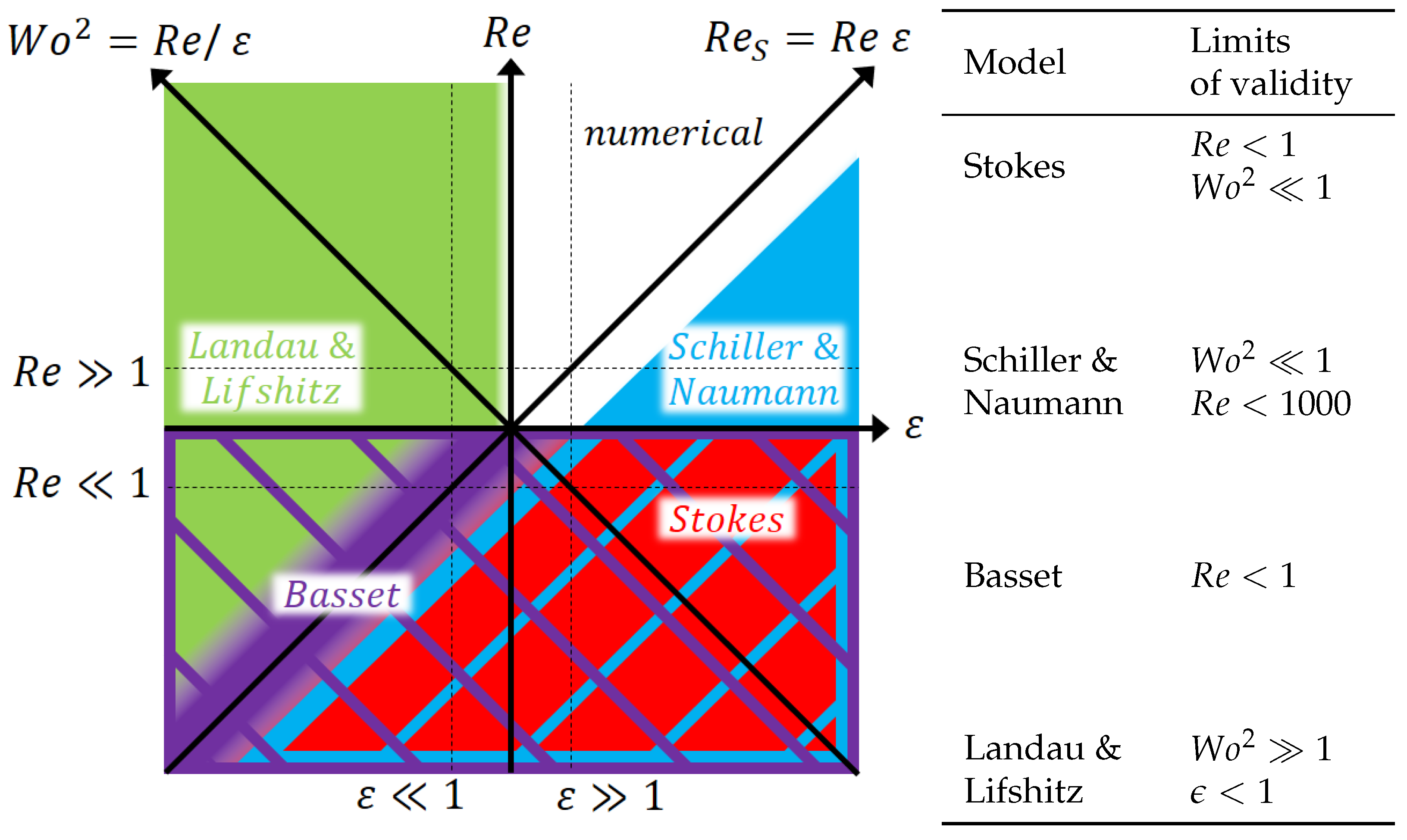
2.1. Drag Models
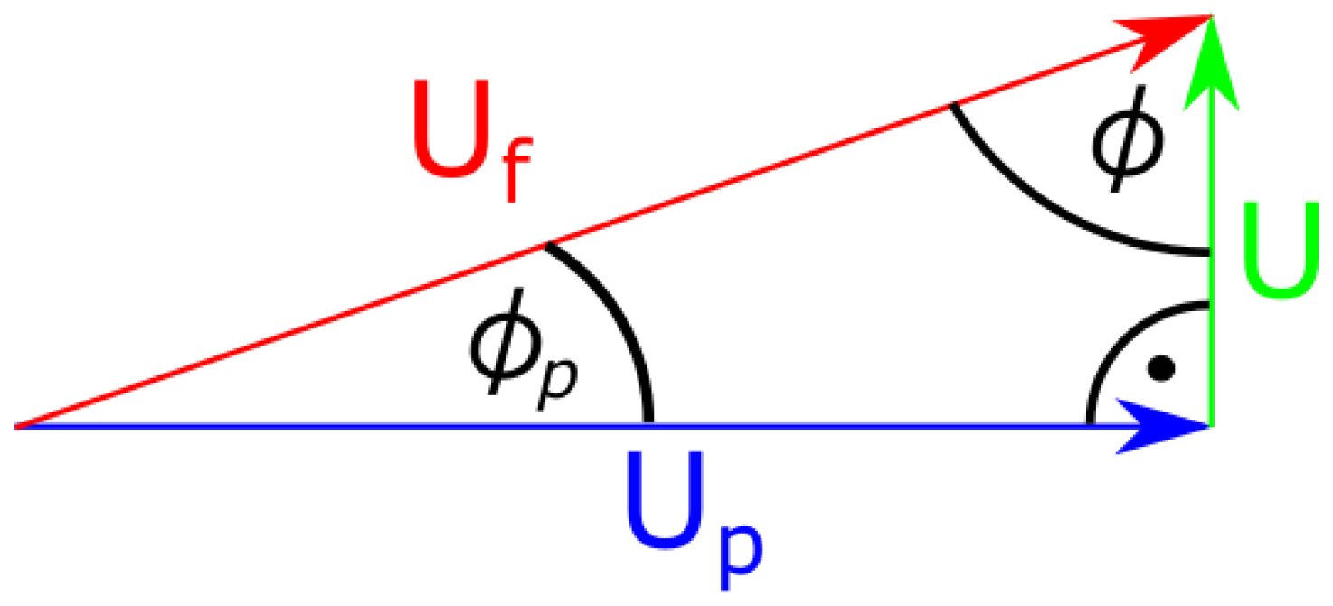
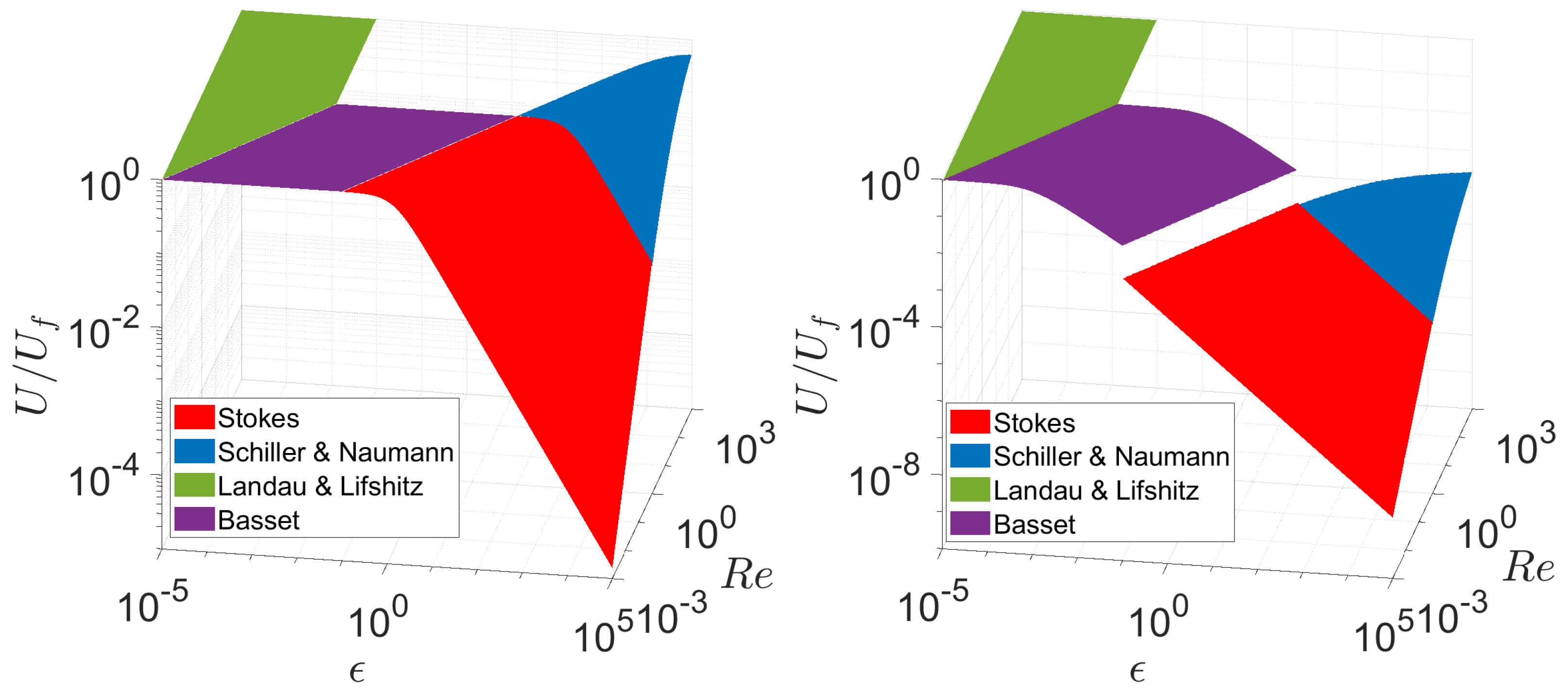
2.2. Slip Velocity Amplitude
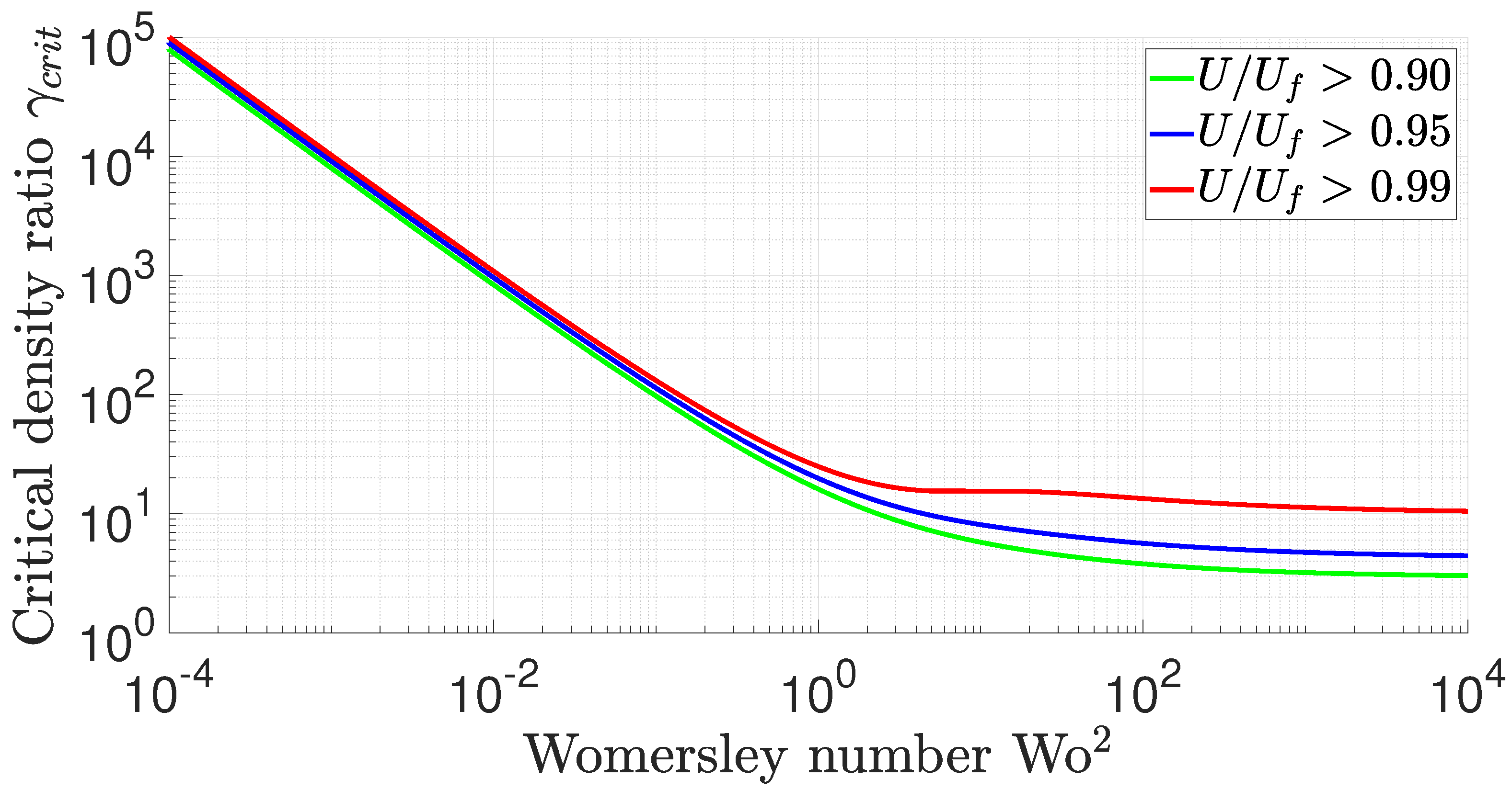
2.3. Particle Relaxation
3. Result and Discussion
4. Conclusions
Author Contributions
Funding
Data Availability Statement
Conflicts of Interest
Nomenclature
| A | displacement amplitude |
| a | particle acceleration |
| drag coefficient | |
| d | particle diameter |
| F | force |
| Reynolds number | |
| oscillation Stokes number | |
| t | time |
| u | velocity |
| U | velocity amplitude |
| Womersley number (frequency parameter) | |
| density ratio | |
| amplitude parameter | |
| dynamic viscosity | |
| density | |
| relaxation time | |
| phase shift | |
| angular frequency | |
| Abbreviations | |
| Landau & Lifshitz | |
| Navier-Stokes equations | |
| ordinary differential equation | |
| S | Stokes |
| Schiller & Naumann | |
| standard temperature and pressure | |
| Indices | |
| D | drag |
| I | inertia |
| p | particle |
| f | fluid |
| 0 | initial state |
Appendix A. Derivation of the Slip Velocity Amplitude Calculated with the Stokes Drag Model
Appendix B. Derivation of Slip Velocity Amplitude Calculated with SN and Deviation from the Stokes Model
Appendix C. Derivation and Solution of Particle Motion with the Landau & Lifshitz Model
References
- Rothlisberger, M.; Schmidli, G.; Schuck, M.; Kolar, J.W. Multi-Frequency Acoustic Levitation and Trapping of Particles in All Degrees of Freedom. IEEE Trans. Ultrason. Ferroelectr. Freq. Control 2022, 69, 1572–1575. [Google Scholar] [CrossRef] [PubMed]
- Wang, Y.; Wu, L.; Wang, Y. Study on Particle Manipulation in a Metal Internal Channel under Acoustic Levitation. Micromachines 2021, 13, 18. [Google Scholar] [CrossRef] [PubMed]
- Heidinger, S.; Spranger, F.; Dostál, J.; Zhang, C.; Klaus, C. Material Treatment in the Pulsation Reactor—From Flame Spray Pyrolysis to Industrial Scale. Sustainability 2022, 14, 3232. [Google Scholar] [CrossRef]
- Klaus, C.; Wegner, K.; Rammelt, T.; Ommer, M. New Challenges in Thermal Processing. Interceram Int. Ceram. Rev. 2021, 70, 22–25. [Google Scholar] [CrossRef]
- Hoffmann, C.; Ommer, M. Reactors for fluid-solid reactions: Pulsation reactors. In Handbuch Chemische Reaktoren; Reschetilowski, W., Ed.; Springer Reference Naturwissenschaften; Springer: Berlin/Heidelberg, Germany, 2019; pp. 1–19. [Google Scholar] [CrossRef]
- Hjelmfelt, A.T.; Mockros, L.F. Motion of discrete particles in a turbulent fluid. Appl. Sci. Res. 1966, 16, 149–161. [Google Scholar] [CrossRef]
- Womersley, J.R. Method for the calculation of velocity, rate of flow and viscous drag in arteries when the pressure gradient is known. J. Physiol. 1955, 127, 553–563. [Google Scholar] [CrossRef] [PubMed]
- Clift, R.; Grace, J.R.; Weber, M.E. Bubbles, Drops, and Particles; Dover Publications: Mineola, NY, USA, 2013. [Google Scholar]
- Riley, N. On a Sphere Oscillating in a Viscous Fluid. Q. J. Mech. Appl. Math. 1966, 19, 461–472. [Google Scholar] [CrossRef]
- Riley, N. Steady Streaming. Annu. Rev. Fluid Mech. 2001, 33, 43–65. [Google Scholar] [CrossRef]
- Landau, L.D.; Lifshitz, E.M. Fluid Mechanics, 2nd ed.; Course of Theoretical Physics; Pergamon: Oxford, UK, 1987; Volume 6. [Google Scholar]
- Stokes, G.G. On the Effect of the Internal Friction of Fluids on the Motion of Pendulums. In Mathematical and Physical Papers; Cambridge University Press: Cambridge, UK, 2009; pp. 1–10. [Google Scholar] [CrossRef]
- Schiller, L.; Naumann, A. VDI Zeitung; VDI: Düsseldorf, Germany, 1935. [Google Scholar]
- Goossens, W.R. Review of the empirical correlations for the drag coefficient of rigid spheres. Powder Technol. 2019, 352, 350–359. [Google Scholar] [CrossRef]
- Basset, A.B. On the motion of a sphere in a viscous liquid. Philos. Trans. R. Soc. Lond. (A) 1888, 179, 43–63. [Google Scholar] [CrossRef] [Green Version]
- Coimbra, C.F.M.; Rangel, R.H. Spherical Particle Motion in Harmonic Stokes Flows. AIAA J. 2001, 39, 1673–1682. [Google Scholar] [CrossRef]
- Sazhin, S.; Shakked, T.; Sobolev, V.; Katoshevski, D. Particle grouping in oscillating flows. Eur. J. Mech. B/Fluids 2008, 27, 131–149. [Google Scholar] [CrossRef]


| Name | Drag Force | Slip Velocity Amplitude Ratio | |
|---|---|---|---|
| Stokes | |||
| Schiller & Naumann | |||
| Basset | |||
| Landau & Lifshitz | |||
| Name | Relation to Stokes | ||
|---|---|---|---|
| Schiller & Naumann | |||
| Basset | ∧ | ||
| Landau & Lifshitz | |||
Publisher’s Note: MDPI stays neutral with regard to jurisdictional claims in published maps and institutional affiliations. |
© 2022 by the authors. Licensee MDPI, Basel, Switzerland. This article is an open access article distributed under the terms and conditions of the Creative Commons Attribution (CC BY) license (https://creativecommons.org/licenses/by/4.0/).
Share and Cite
Heidinger, S.; Unz, S.; Beckmann, M. Simple Particle Relaxation Modeling in One-Dimensional Oscillating Flows. Processes 2022, 10, 1322. https://doi.org/10.3390/pr10071322
Heidinger S, Unz S, Beckmann M. Simple Particle Relaxation Modeling in One-Dimensional Oscillating Flows. Processes. 2022; 10(7):1322. https://doi.org/10.3390/pr10071322
Chicago/Turabian StyleHeidinger, Stefan, Simon Unz, and Michael Beckmann. 2022. "Simple Particle Relaxation Modeling in One-Dimensional Oscillating Flows" Processes 10, no. 7: 1322. https://doi.org/10.3390/pr10071322