Study on Piezomagnetic Effect of Iron Cobalt Alloy and Force Sensor

Abstract

Based on the nonlinear piezomagnetic equation, the piezomagnetic effect of prismatic iron-cobalt alloy is analyzed by using the ANSYS finite element simulation platform. The variation of the dynamic piezomagnetic coefficient of the iron-cobalt alloy under different bias magnetic fields and different stress was studied through simulation. Referring to the working condition of the tractor force sensor and according to the principle of magnetic circuit superposition, a piezomagnetic force sensor was designed and manufactured using iron-cobalt alloy. According to the electromagnetic theory and piezomagnetic effect, the three-dimensional model and magnetic circuit mathematical model of the sensor are established, and the system simulation model of the piezomagnetic sensor was established based on the MATLAB/Simulink module. The experimental platform of the magnetostrictive force sensor was built to verify the correctness of the simulation model, and the effects of bias magnetic field and force on the output characteristics are studied. The simulation and experimental results show that the maximum piezomagnetic coefficient was 9.2 T/GPA when the bias magnetic field intensity was 14.74 kA/m. The force measuring range of the sensor is 0–120 kN, and the sensor has high sensitivity within 0–80 kN. The sensor has a simple structure, is suitable for the force measurement and control of an electro-hydraulic lifter under heavy load, and can better adapt to the harsh working environment.

1. Introduction

Iron-cobalt alloy is an important metal soft magnetic material with good magnetic properties and high magneto-mechanical coupling coefficient, which has high Curie temperature and saturated magnetic induction intensity at room temperature. It also has the advantages of high permeability and low coercivity [1,2,3,4,5]. Compared with rare earth magnetostrictive material (Terfenol-D) and piezoelectric material, the iron-cobalt alloy has better magnetic stability [6,7]. It is widely used in transformers, motors, telephone diaphragms, embedded iron of high-speed printers, receiver coil, switches, and storage iron core current transformers (see transformer) [8]. Magnetostrictive displacement sensors [9], magnetostrictive strain sensors [10], and magnetostrictive pressure sensors [11] can be developed by using the piezomagnetic effect of the iron-cobalt alloy.

The piezomagnetic coefficient refers to the change of magnetic induction intensity of magnetostrictive material caused by unit stress, so the piezomagnetic coefficient is closely related to the sensitivity of the magnetostrictive pressure sensor [12,13]. Tong Jie, the Chinese Academy of Electric Power Sciences, and others designed a saw current transformer based on the magnetostrictive effect of iron-cobalt materials [14]. Yang et al. deduced the relationship of piezomagnetic coefficient and bias magnetic field under zero stress by using a magnetostrictive nonlinear constitutive model and determined the influence law of bias magnetic field on magnetoelectric effect and vibration frequency of magnetostrictive materials [15]. In the literature [16], the effect of compressive and tensile stress on the piezomagnetic coefficient was studied. The experimentally obtained piezomagnetic coefficient could then be obtained through the fitting of the appropriate data. Cui et al. [17] and others designed a force sensor using flake iron calcium alloy and iron-cobalt alloy materials, revealing the physical mechanism of the magnetostrictive force sensor and the influencing factors of sensor output characteristics.

Based on the nonlinear piezomagnetic equation, this paper studies the influence of stress and bias magnetic field on piezomagnetic effect by using finite element simulation software, analyzes the variation law of piezomagnetic coefficient as a function of stress and bias magnetic field, and obtains the bias magnetic field corresponding to the maximum piezomagnetic coefficient under each stress. In view of the more and more extensive application of high-power tractors in modern agricultural machinery, the current tractor lift force sensor cannot meet the needs of the harsh working environment, referring to the working conditions of the tractor force sensor [18,19,20], a piezomagnetic effect force sensor [21,22,23,24,25] is designed and manufactured for the detection of elevator force of large tractor.

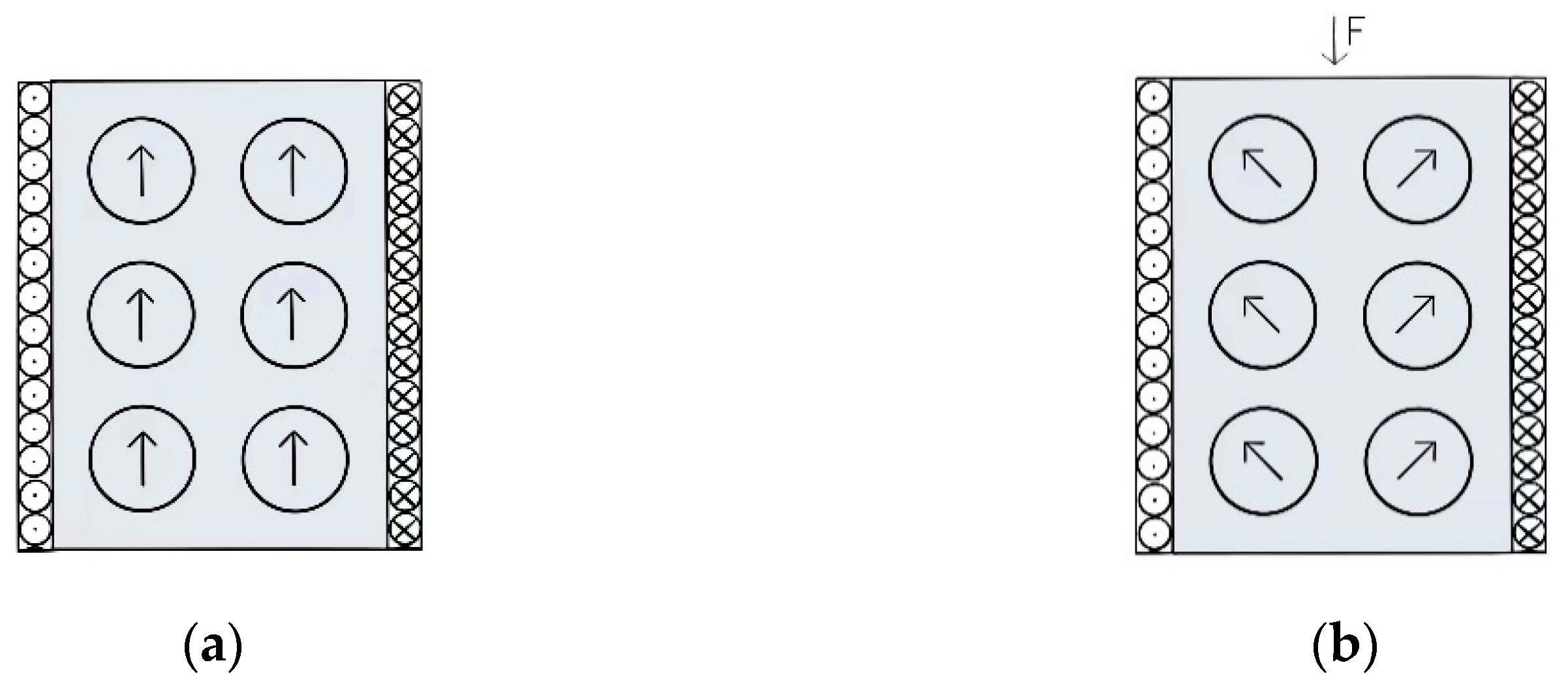
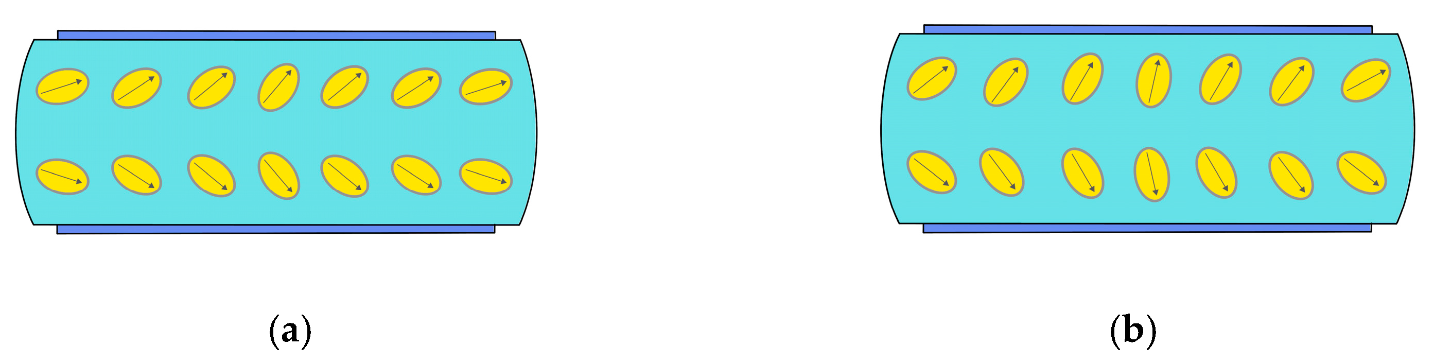
2. Principle and Model of Piezomagnetic Effect

The piezomagnetic effect means that when a material is subjected to an external force, the internal stress changes the magnetization of the material. Concomitantly the material permeability will also change. Magnetostriction can be explained by domain theory from the microscopic point of view. For ferromagnetic materials, its interior can be regarded as composed of several magnetized regions, and each small, magnetized region is called a magnetic domain. When the ferromagnetic material is not magnetized, the magnetic moment of each small magnetic domain is evenly distributed in all directions. When the ferromagnetic material is affected by the magnetic field, the internal magnetic domain will deflect under the action of the external magnetic field, and the deflection of the magnetic domain affects the magnetization [5]. This characteristic of magnetostrictive materials can be used to convert mechanical signals into magnetic signals.

When the prismatic iron-cobalt alloy material used in this study is subjected to a force perpendicular to the surface as shown in Figure 1, the internal magnetic domain will change due to the applied stress. The coil with DC current provides a bias magnetic field along the axial direction for the prismatic iron-cobalt alloy material. Figure 1a shows that when the iron-cobalt alloy is not stressed, the magnetic domain directions on the alloy section are arranged along the direction of the bias magnetic field. Figure 1b shows that when a force F is applied along the direction of the applied magnet, and perpendicular to the circular surface, as indicated in Figure 1b, the magnetic domain structure in the iron-cobalt will change in response to the applied force, resulting in the reduction of its internal average magnetic induction intensity.

Based on the piezomagnetic equation of magnetostrictive materials, the magnetic induction intensity can be expressed as [26].

$$B=d_{33}^{*}\sigma +\mu H$$

(1)

where, B is the magnetic induction intensity in the iron-cobalt alloy; $d^{*}{}_{33}$ is the piezomagnetic coefficient; σ is the stress; μ is permeability; H is the bias magnetic field strength. The magnetic induction intensity B is affected by the magnetic field and stress with the bias magnetic field intensity H and σ. The piezomagnetic coefficient $d^{*}{}_{33}$ is also affected by the bias magnetic field H and stress σ.

The piezomagnetic coefficient can directly reflect the magneto-mechanical conversion efficiency of iron-cobalt alloy and affect the output characteristics of the sensor. The larger the piezomagnetic coefficient, the greater the change of magnetic induction intensity of iron-cobalt alloy caused by unit stress. In order to obtain iron-cobalt alloy piezomagnetic coefficient $d^{*}{}_{33}$ and the bias magnetic field H and stress σ. In the nonlinear constitutive model proposed in reference [27], the model formula of iron-cobalt alloy is derived:

$$\epsilon =\frac{\sigma }{E}+{\lambda }_0(\sigma )+\frac{{\lambda }_{\mathrm{s}}-{\lambda }_0(\sigma )}{M_{\mathrm{s}}^2}{M}^2$$

(2)

$$H=\frac{1}{\eta }{f}^{-1}\left(\frac{M}{M_{\mathrm{s}}}\right)-\frac{2\left({\lambda }_{\mathrm{s}}\sigma -{\mathsf{\Lambda }}_0(\sigma )\right)}{{\mu }_0{M}_{\mathrm{s}}^2}M$$

(3)

Among

$${\lambda }_0(\sigma )={\lambda }_{\mathrm{s}}\{\begin{array}{ll}\tanh \frac{\sigma }{{\sigma }_{\mathrm{s}}}\hfill & \sigma ⩾0\hfill \\ \tanh \frac{2\sigma }{{\sigma }_{\mathrm{s}}}/2\hfill & \sigma <0\hfill \end{array}$$

$${\mathsf{\Lambda }}_0(\sigma )={\lambda }_{\mathrm{s}}{\sigma }_{\mathrm{s}}\{\begin{array}{ll}\ln \left(\cosh \frac{\sigma }{{\sigma }_{\mathrm{s}}}\right)\hfill & \sigma ⩾0\hfill \\ \ln \left(\cosh \frac{2\sigma }{{\sigma }_{\mathrm{s}}}\right)/4\hfill & \sigma <0\hfill \end{array}$$

$$f(x)=\coth x-\frac{1}{x} \eta =\frac{3{\chi }_{\mathrm{m}}}{M_{\mathrm{s}}}$$

where, ɛ is the strain; M is magnetization; Ms is saturation magnetization; λs is the saturation magnetostrictive strain coefficient; ${\chi }_{\mathrm{m}}$ is the initial magnetic susceptibility; σ_s is saturated pre-stress; μ₀ is vacuum permeability; E is Young’s modulus. Based on the principle of electromagnetism, combined with Equation (3), the piezomagnetic coefficient of the iron-cobalt alloy is:

$$d_{33}^{*}=\frac{\mathrm{d}B}{ \mathrm{d}\sigma }=\frac{\mathrm{d}{\mu }_0(H+M)}{\mathrm{d}\sigma }$$

(4)

Formula (2) and Formula (3) show that there is a complex coupling relationship between magnetostriction and magnetization and stress and magnetic field. Therefore, it is of great significance for the design and structural optimization of magnetostrictive sensors to study the influence of bias magnetic field and stress on the piezomagnetic effect of iron-cobalt alloy and to apply the iron-cobalt alloy to large tractor force sensors. This paper solves the dynamic piezomagnetic coefficient $d^{*}{}_{33}$ through the simulation software ANSYS.

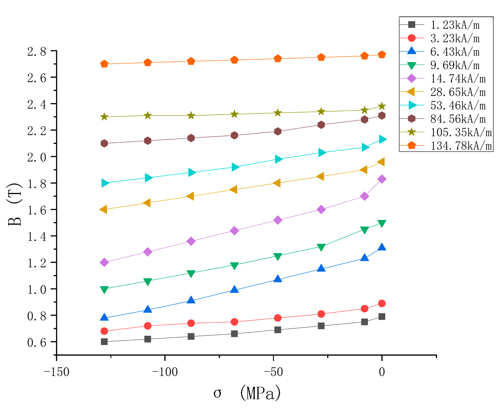
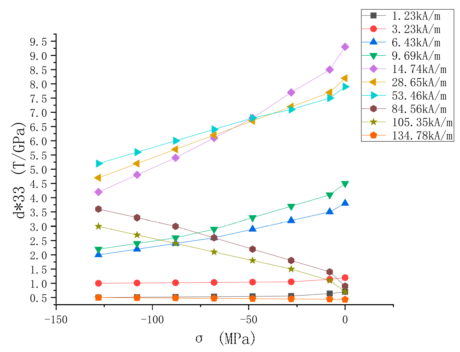
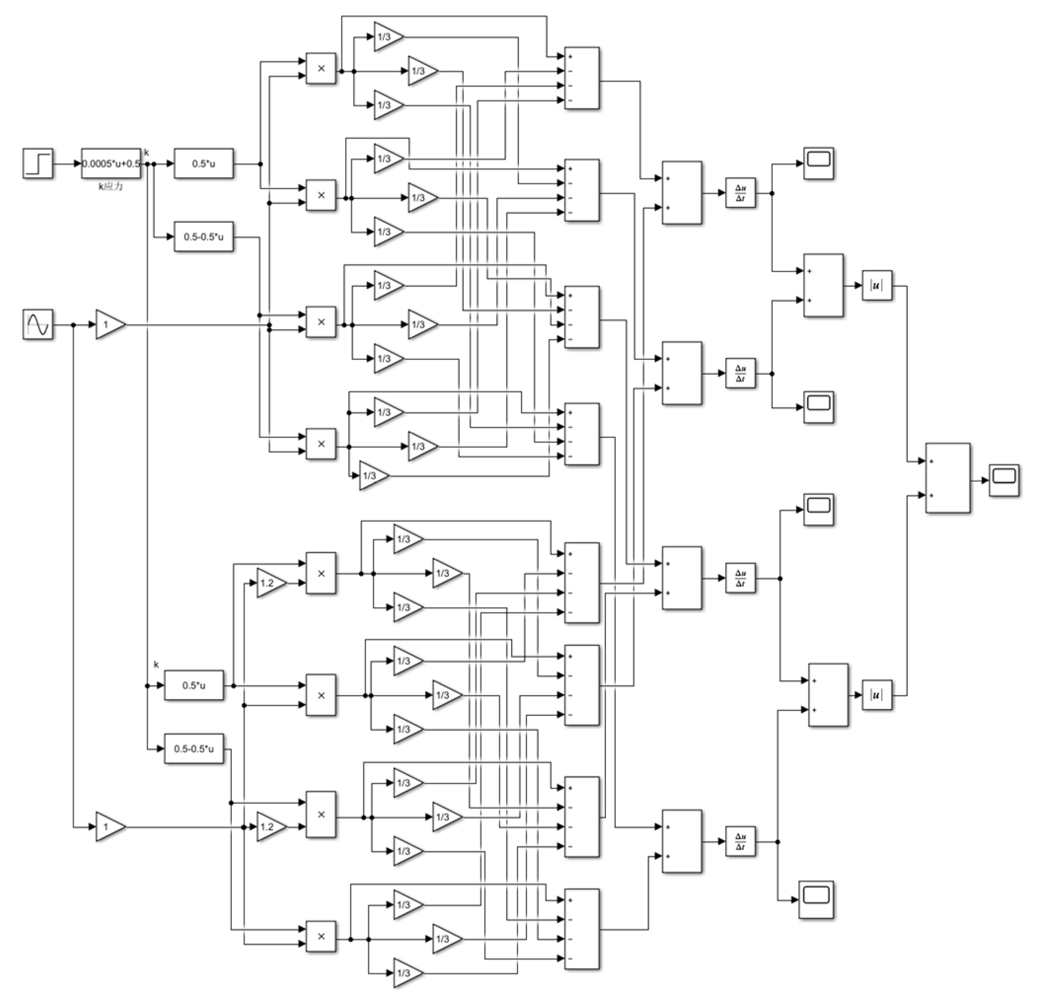
3. Simulation Results and Analysis

The iron-cobalt alloy prism is modeled by ANSYS simulation software. The prism size is 28 mm × 33 mm × 96 mm. By adjusting the coil current to change the bias magnetic field applied to the prism and setting different forces on both sides of the prism, the force working condition of the sensor is simulated, as shown in Figure 2.

In Ansys software, the parameter in Equations (2) and (3) is defined as: M_s = 1.92 ×${10}^6$ A/m, λs = 74 ×${10}^{-6},{\chi }_m$ = 200, σs = 55 MPa, μ₀ = 4π ×${10}^{-7}$ T·m/A, E = 76 ×${10}^9$ Pa [28], the number of turns of the excitation coil is n = 130, the external force is 0 and the coil current is 5A. The magnetic field distribution diagram of the longitudinal section of the prism is obtained by simulation, that is, the simulated magnetic field distribution diagram of the x-z plane, as shown in Figure 3. It can be seen from the figure that the magnetic induction intensity at the center of the iron-cobalt alloy prism is the largest, which can reach 1.4 T, and the magnetic induction intensity gradually decreases from the center to both sides. This is due to the influence of the biased magnetic field generated by the coil. The bias magnetic field in the middle part is larger and the bias magnetic field on both sides is smaller.

Adjusting the solution domain in the Ansys magnetic field module and setting the incoming DC current of the coil to 0–10 A can make the prismatic iron-cobalt alloy produce a magnetic field strength of 0–134.78 kA/m. Adjusting the solution domain in the Ansys solid mechanics module, setting the point load conditions, and applying a force of 0–120 kn at both ends of the prismatic iron-cobalt alloy can produce compressive stress of −128–0 Mpa in the prismatic section. The simulation results show the simulation relationship between magnetic induction intensity and compressive stress under different bi-as magnetic fields, as shown in Figure 4. When the bias magnetic field intensity is less than 3.11 kA/m, the change rate of magnetic induction intensity with compressive stress is small, because the stress has little effect on domain deflection under a weak magnetic field. When the bias magnetic field intensity is in the range of 3.11–84.56 kA/m, the change rate of magnetic induction intensity is large, and the magnetic induction intensity decreases gradually with the increase of compressive stress. When the bias magnetic field intensity is greater than 84.56 kA/m, the change rate of magnetic induction intensity with compressive stress is small, mainly because the influence of stress on domain deflection becomes smaller due to the excessive magnetic field intensity.

By deriving the points in Figure 4, the variation curve of the piezomagnetic coefficient $d^{*}{}_{33}$ and compressive stress under different bias magnetic fields was obtained, as shown in Figure 5. $d^{*}{}_{33}$ is a function of bias magnetic field and stress. By extracting the piezomagnetic coefficient under different stress in Figure 5, the relationship curve between $d^{*}{}_{33}$ and bias magnetic field under different stress is drawn, as shown in Figure 6. Through the analysis of Figure 5 and Figure 6, with the increase of the magnetic field strength, the piezomagnetic coefficient first increases, then decreases, and finally, tends to be stable. This is because the magnetic domain deflection angle of the material first increases according to the increase of the magnetic field strength. After reaching a certain degree, the influence of the magnetic field strength on the magnetic domain begins to decrease. Figure 7a,b show the changes of the same force on the domain deflection direction under the bias magnetic field of 105.35 kA/m and 14.74 kA/m, respectively. Under the bias magnetic field of 14.74 kA/m, the deflection angle of the magnetic domain is larger, so the piezomagnetic coefficient of the material is larger. In addition, with the increase of compressive stress, the maximum value of the piezomagnetic coefficient gradually decreases and shifts to the right. This is because the saturated magnetic field of iron gallium alloy increases with the increase of compressive stress, but the saturated magnetic induction intensity is basically unchanged. Before saturation, the magnetic induction intensity of iron gallium alloy decreases with the rate of change of magnetic field intensity, that is, the permeability decreases. Therefore, there is an optimal bias magnetic field for the magnetostrictive force sensor of a specific material. When the force sensor works at this optimal bias magnetic field, the output voltage and sensitivity of the force sensor reach the maximum. When no stress is applied, the bias magnetic field intensity is 14.74 kA/m, and the piezomagnetic coefficient reaches the maximum value of 9.2 T/GPa. Since the working range of the sensor is mainly 0–80 kN, when the iron-cobalt material is used to design the column sensor, in order to increase the sensitivity of the sensor, the bias magnetic field corresponding to the maximum value of piezomagnetic coefficient should be selected, that is, 14.74 kA/m.

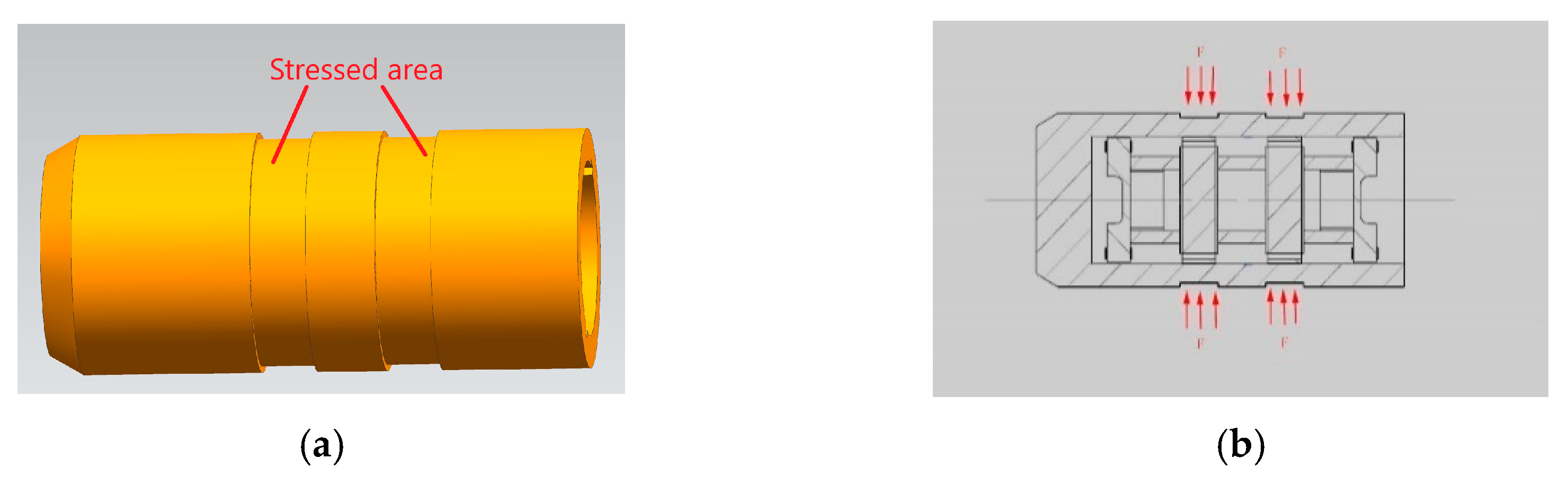
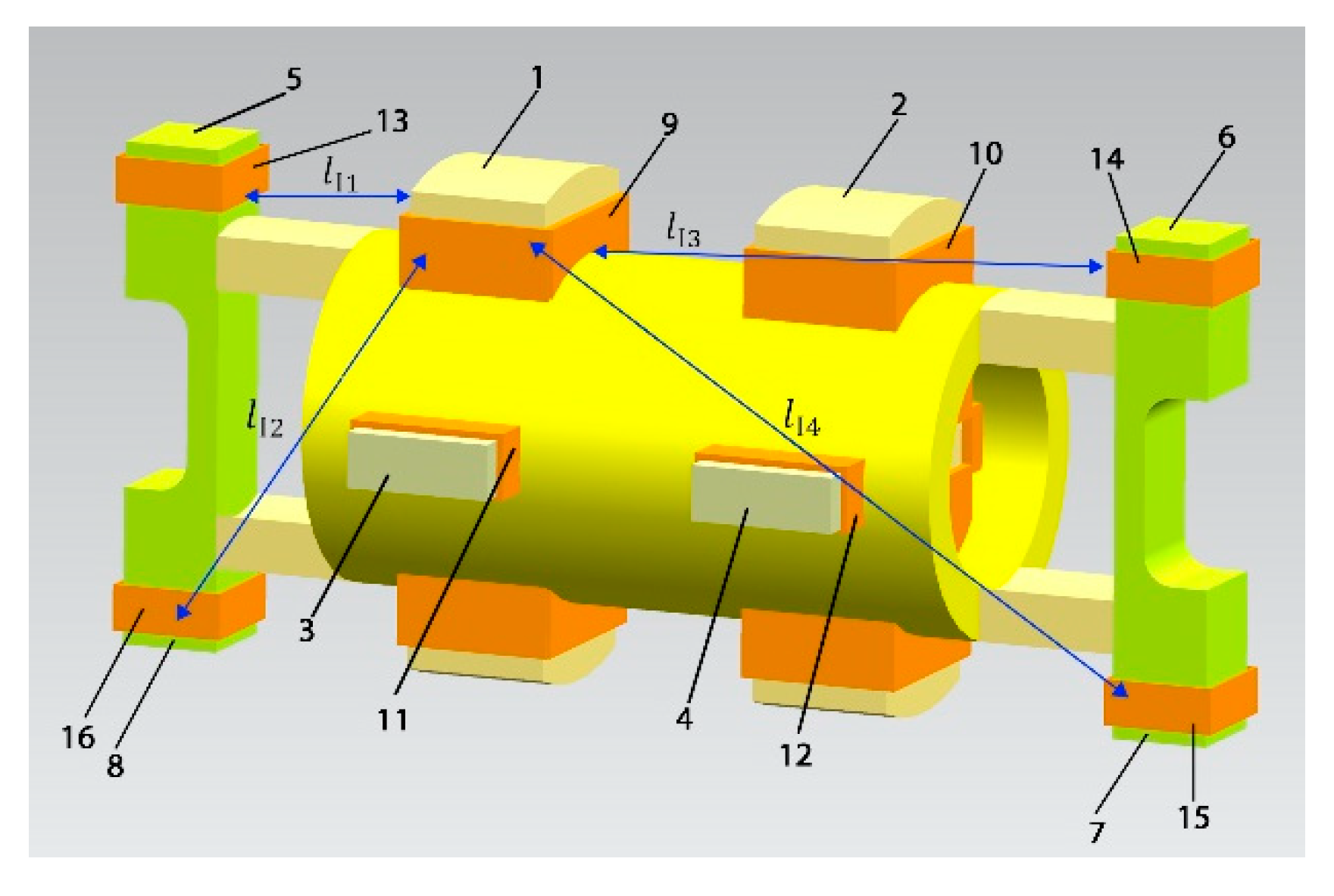
4. Design of Magnetostrictive Force Sensor

Sensor Structure

According to the working conditions of the tractor lifter, referring to the KMB force sensor [29] on the market, a new piezomagnetic sensor, which is an improvement based on KMB, is designed by using iron-cobalt material to improve the defect that the KMB sensor can only receive one-directional force and has insufficient sensitivity. The sensor can be installed on the lifter through a suit. When the sensor is working, the external radial force along the sleeve acts on the sensor through the groove on the sleeve, and then the sleeve transmits the force to the iron-cobalt alloy. The sensor assembly and its stress diagram are shown in Figure 8. The sensor structure is shown in Figure 9.

The working principle of the sensor is: under no-load conditions, a symmetrical magnetic field is formed through the primary coil between the excitation cores; when the sensor is subjected to external force, the permeability of the horizontal excitation magnetic core and the vertical excitation magnetic core changes, resulting in the change of the magnetic field and becoming an asymmetric state, resulting in the change of the magnetic flux passing through each induction magnetic core, the magnetic potential difference is formed between the secondary coils, so that the magnetic flux flows through the secondary circuit, resulting in the output voltage on the induction coil after differential connection, which reflects the size of the external force. The magnetic fields generated by vertical excitation core I and vertical excitation core II and horizontal excitation core I and horizontal excitation core II of the piezomagnetic force sensor designed in this paper are superimposed with each other, which increases the magnetic flux in the induction coil, together they constitute the output signal of the sensor and increase the sensitivity of the sensor.

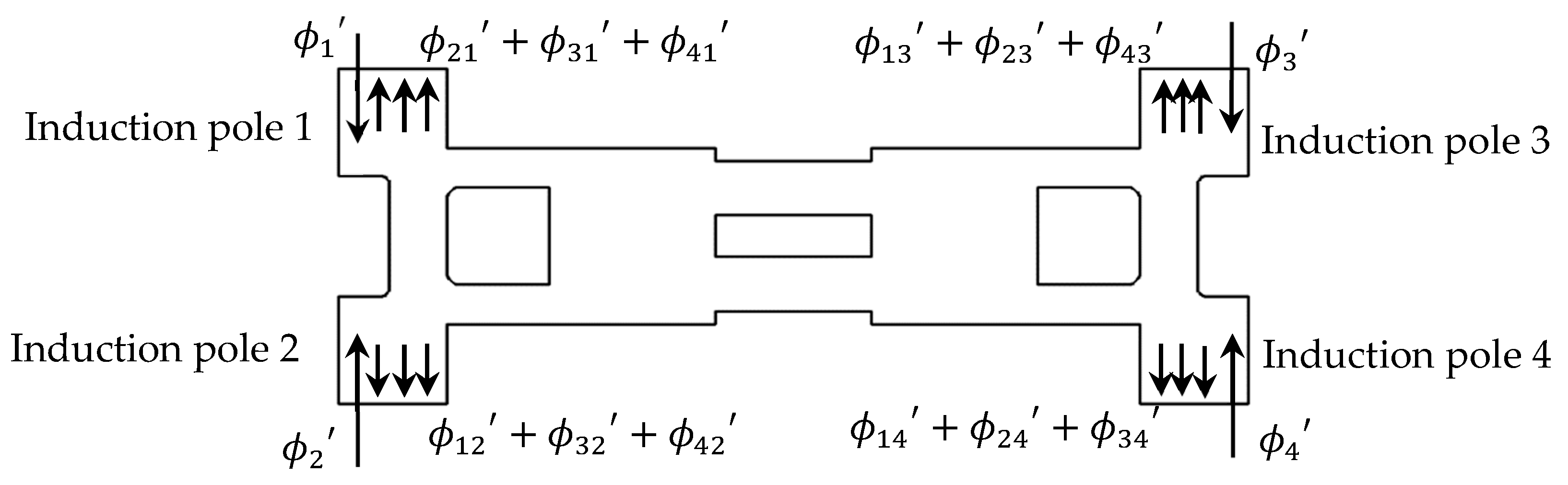
5. Mathematical Analysis of Magnetic Circuit

Figure 10 shows the schematic diagram of the magnetic circuit. The magnetomotive force generated by the excitation core includes two parts: the magnetomotive force $F_{\mathit{Mz}}$ generated by the vertical coil and the magnetomotive force $F_{\mathit{Mp}}$ generated by the horizontal coil. The horizontal coil axis and the induction magnetic pole axis are located on the same plane, and the magnetic flux direction is parallel to the plane. The coil axis in the vertical direction is perpendicular to the axis of the induction magnetic pole, and its magnetic flux direction is perpendicular to the plane where the axis of the induction magnetic pole is located so that the number of turns of the winding coils in the horizontal and vertical directions of the two excitation magnetic cores is n, and the coils in the horizontal and vertical directions of each excitation magnetic core are connected in series, and the two excitation magnetic cores are connected in series:

$$F_{MZ}=F_{MP}=NI, F_M=F_{MZ}+F_{MP}=2NI$$

(5)

where $I$—excitation current, $F_M$—total magnetomotive force of each excitation core

5.1. Horizontal Magnetic Circuit Structure

For the excitation pole in the horizontal direction, the total flux generated by the magnetomotive force of the excitation coil in the horizontal direction without considering the influence of magnetic leakage—${\varphi }_{0p}$—enters four induction magnetic poles through the sleeve:

$${\varphi }_{0p}={\varphi }_{1p}+{\varphi }_{2p}+{\varphi }_{3p}+{\varphi }_{4p}$$

(6)

${\varphi }_{np}$—Magnetic flux flowing from the excitation core to the induction pole n in the horizontal direction (n = 1, 2, 3, 4).

Because the structure is symmetrical, the I excitation core is analyzed first: As shown in Figure 10, the distance between induction pole 1 and induction pole 2 from the excitation core is close, and the magnetic flux is large. The distance between induction pole 3 and induction pole 4 from the excitation core is far, and the magnetic flux is small.

$${\varphi }_{\mathrm{I}1p}={\varphi }_{\mathrm{I}2p}>{\varphi }_{\mathrm{I}3p}={\varphi }_{\mathrm{I}4p}$$

(7)

where ${\varphi }_{\mathrm{I}np}$—Magnetic flux flowing from excitation core I to induction pole n in the horizontal direction (n = 1, 2, 3, 4).

Among them, the magnetic flux ${\varphi }_{\mathrm{I}1p}$ flowing through the induction magnetic pole 1 is conducted through the intermediate magnetic circuit and returns to the excitation magnetic core through the other three induction magnetic poles to form a complete magnetic circuit:

$${\varphi }_{\mathrm{I}1p}={\varphi }_{\mathrm{I}12p}+{\varphi }_{\mathrm{I}13p}+{\varphi }_{\mathrm{I}14p}$$

(8)

where ${\varphi }_{\mathrm{I}np}$—Magnetic flux (n = 1, 2, 3, 4) generated by horizontal I excitation core from induction pole 1 to induction pole n. From Ohm’s law of magnetic circuit:

$${\varphi }_{\mathrm{I}1p}=\frac{F_{MP}}{R_Z}=\frac{NI}{R_1+R_0+R_M+R_2//R_3//R_4}$$

(9)

where $R_n$—Magnetoresistance of induction pole n (n = 1, 2, 3, 4); $R_M$—Magnetoresistance of excitation core; $R_0$—the total magnetoresistance of other parts in the magnetic circuit, including the sleeve and its connection with the excitation core and the induction core;$R_Z$—total reluctance of magnetic circuit.

Similarly, for the flux ${\varphi }_{np}$ flowing from the I horizontal excitation core to other induction poles, there is:

$$\{\begin{array}{c}{\varphi }_{\mathrm{I}2p}=\frac{F_{MP}}{R_Z}=\frac{NI}{R_2+R_0+R_M+R_1//R_3//R_4}\\ {\varphi }_{\mathrm{I}3p}={\varphi }_{\mathrm{I}31p}+{\varphi }_{\mathrm{I}32p}+{\varphi }_{\mathrm{I}34p}\\ {\varphi }_{\mathrm{I}3p}=\frac{F_{MP}}{R_Z}=\frac{NI}{R_3+R_0+R_M+R_2//R_1//R_4}\\ {\varphi }_{\mathrm{I}4p}={\varphi }_{\mathrm{I}41p}+{\varphi }_{\mathrm{I}42p}+{\varphi }_{\mathrm{I}43p}\\ {\varphi }_{\mathrm{I}4p}=\frac{F_{MP}}{R_Z}=\frac{NI}{R_4+R_0+R_M+R_2//R_1//R_3}\end{array}$$

(10)

This is the magnetic flux generated by the horizontal excitation core I. Similarly, according to the principle of symmetry, the magnetic flux generated by the horizontal excitation core II for No. 1, 2, 3, and 4 induction poles is obtained:

$$\{\begin{array}{c}{\varphi }_{\mathrm{II}3p}={\varphi }_{\mathrm{II}4p}>{\varphi }_{\mathrm{II}1p}={\varphi }_{\mathrm{II}2p}\\ {\varphi }_{\mathrm{II}12p}={\varphi }_{\mathrm{II}13p}={\varphi }_{\mathrm{II}14p}=\frac{{\varphi }_{\mathrm{II}1p}}{3}=\frac{{\varphi }_{\mathrm{I}3p}}{3}\\ {\varphi }_{\mathrm{II}21p}={\varphi }_{\mathrm{II}23p}={\varphi }_{\mathrm{II}24p}=\frac{{\varphi }_{\mathrm{II}2p}}{3}=\frac{{\varphi }_{\mathrm{I}4p}}{3}\\ {\varphi }_{\mathrm{II}31p}={\varphi }_{\mathrm{II}32p}={\varphi }_{\mathrm{II}34p}=\frac{{\varphi }_{\mathrm{II}3p}}{3}=\frac{{\varphi }_{\mathrm{I}1p}}{3}\\ {\varphi }_{\mathrm{II}41p}={\varphi }_{\mathrm{II}42p}={\varphi }_{\mathrm{II}43p}=\frac{{\varphi }_{\mathrm{II}4p}}{3}=\frac{{\varphi }_{\mathrm{I}2p}}{3}\end{array}$$

(11)

The magnetic flux generated by the horizontal excitation coil and passing through each induction pole is:

$$\{\begin{array}{c}{\varphi }_{10p}={\varphi }_{\mathrm{I}1p}+{\varphi }_{\mathrm{II}1p}-({\varphi }_{\mathrm{I}21p}+{\varphi }_{\mathrm{I}31p}+{\varphi }_{\mathrm{I}41p})-({\varphi }_{\mathrm{II}21p}+{\varphi }_{\mathrm{II}41p}+{\varphi }_{\mathrm{II}31p})=0\\ {\varphi }_{20p}={\varphi }_{\mathrm{I}2p}+{\varphi }_{\mathrm{II}2p}-{\varphi }_{\mathrm{I}12p}+{\varphi }_{\mathrm{I}32p}+{\varphi }_{\mathrm{I}42p}-{\varphi }_{\mathrm{II}12p}+{\varphi }_{\mathrm{II}42p}+{\varphi }_{\mathrm{II}32p}=0\\ {\varphi }_{30p}={\varphi }_{\mathrm{I}3p}+{\varphi }_{\mathrm{II}3p}-({\varphi }_{\mathrm{I}13p}+{\varphi }_{\mathrm{I}23p}+{\varphi }_{\mathrm{I}43p})-({\varphi }_{\mathrm{I}13p}+{\varphi }_{\mathrm{I}43p}+{\varphi }_{\mathrm{I}23p})= 0\\ {\varphi }_{40p}={\varphi }_{\mathrm{I}4p}+{\varphi }_{\mathrm{I}4p}-({\varphi }_{\mathrm{I}14p}+{\varphi }_{\mathrm{I}24p}+{\varphi }_{\mathrm{I}34p})-({\varphi }_{\mathrm{II}14p}+{\varphi }_{\mathrm{II}34p}+{\varphi }_{\mathrm{II}24p})=0\end{array}$$

(12)

It can be seen that the total magnetic flux generated by the horizontal excitation coil of I and II excitation cores and passing through each induction pole is:

$$\{\begin{array}{c}{\phi }_{10p}=0\\ {\phi }_{20p}=0\\ {\phi }_{30p}=0\\ {\phi }_{40p}=0\end{array}$$

(13)

5.2. Vertical Magnetic Circuit Structure

For the vertical excitation magnetic pole, it can be seen from Figure 9 that the distance from its N pole to the four induction magnetic poles is not equal, where:

$$l_{\mathrm{I}1}>l_{\mathrm{I}2}>l_{\mathrm{I}3}>l_{\mathrm{I}4}$$

(14)

$l_{\mathrm{I}n}$—Distance between vertical I excitation core and induction pole (n = 1, 2, 3, 4).

Therefore, the magnetic flux generated by the I vertical excitation core on the four induction poles is:

$${\varphi }_{\mathrm{I}1z}>{\varphi }_{\mathrm{I}2z>}{\varphi }_{\mathrm{I}3z>}{\varphi }_{\mathrm{I}4z}$$

(15)

where, ${\varphi }_{\mathrm{I}\mathit{mnz}}$—The magnetic flux generated by the excitation core I in the vertical direction from the induction pole m to the induction pole n, (m, n = 1, 2, 3, 4). Due to the symmetry of the induction core structure, the magnetic flux from one induction pole to the other three induction poles can be equal, that is:

$${\{\begin{array}{c}{\varphi }_{\mathrm{I}12z}={\varphi }_{\mathrm{I}13z}={\varphi }_{14z}=\frac{{\varphi }_{\mathrm{I}1z}}{3}\\ {\varphi }_{\mathrm{I}21z}={\varphi }_{\mathrm{I}23z}={\varphi }_{\mathrm{I}24z}=\frac{{\varphi }_{\mathrm{I}2z}}{3}\\ {\varphi }_{\mathrm{I}31z}={\varphi }_{\mathrm{I}32z}={\varphi }_{\mathrm{I}34z}=\frac{{\varphi }_{\mathrm{I}3z}}{3}\\ {\varphi }_{\mathrm{I}41z}={\varphi }_{\mathrm{I}42z}={\varphi }_{\mathrm{I}43z}=\frac{{\varphi }_{\mathrm{I}4z}}{3}\end{array}}_{}$$

(16)

Similarly, the magnetic flux generated by the No. II excitation core through the four induction poles is:

$$\{\begin{array}{c}{\varphi }_{\mathrm{II}34z}={\varphi }_{\mathrm{II}31z}={\varphi }_{\mathrm{II}32z}=\frac{{\varphi }_{\mathrm{II}3z}}{3}=\frac{{\varphi }_{\mathrm{I}1z}}{3}\\ {\varphi }_{\mathrm{II}43z}={\varphi }_{\mathrm{II}42z}={\varphi }_{\mathrm{II}41z}=\frac{{\varphi }_{\mathrm{II}4z}}{3}=\frac{{\varphi }_{\mathrm{I}2z}}{3}\\ {\varphi }_{\mathrm{II}12z}={\varphi }_{\mathrm{II}13z}={\varphi }_{\mathrm{II}14z}=\frac{{\varphi }_{\mathrm{II}1z}}{3}=\frac{{\varphi }_{\mathrm{I}3z}}{3}\\ {\varphi }_{\mathrm{II}21z}={\varphi }_{\mathrm{II}23z}={\varphi }_{\mathrm{II}24z}=\frac{{\varphi }_{\mathrm{II}2z}}{3}=\frac{{\varphi }_{\mathrm{I}4z}}{3}\end{array}$$

(17)

The total magnetic flux generated by the vertical excitation coils I and II and passing through each induction pole is:

$$\{\begin{array}{c}{\varphi }_{10z}={\varphi }_{\mathrm{I}1z}+{\varphi }_{\mathrm{II}1z}-({\varphi }_{\mathrm{I}21z}+{\varphi }_{\mathrm{I}31z}+{\varphi }_{\mathrm{I}41z})-({\varphi }_{\mathrm{II}21z}+{\varphi }_{\mathrm{II}41z}+{\varphi }_{\mathrm{II}31z})\\ {\varphi }_{20z}={\varphi }_{\mathrm{I}2z}+{\varphi }_{\mathrm{II}2z}-({\varphi }_{\mathrm{I}12z}+{\varphi }_{\mathrm{I}32z}+{\varphi }_{\mathrm{I}42z})-({\varphi }_{\mathrm{II}12z}+{\varphi }_{\mathrm{II}42z}+{\varphi }_{\mathrm{II}32z})=- {\varphi }_{10z}\\ {\varphi }_{30z}={\varphi }_{\mathrm{I}3z}+{\varphi }_{\mathrm{II}3z}-{\varphi }_{\mathrm{I}13z}+{\varphi }_{\mathrm{I}23z}+{\varphi }_{\mathrm{I}43z}-{\varphi }_{\mathrm{II}13z}+{\varphi }_{\mathrm{II}43z}+{\varphi }_{\mathrm{II}23z}= {\varphi }_{10z}\\ {\varphi }_{40z}={\varphi }_{\mathrm{I}4z}+{\varphi }_{\mathrm{II}4z}-({\varphi }_{\mathrm{I}14z}+{\varphi }_{\mathrm{I}24z}+{\varphi }_{\mathrm{I}34z})-({\varphi }_{\mathrm{II}14z}+{\varphi }_{\mathrm{II}34z}+{\varphi }_{\mathrm{II}24z})=- {\varphi }_{10z}\end{array}$$

(18)

The magnetic field actions in the horizontal and vertical directions are superimposed on each other, and the total magnetic flux passing through each induced magnetic pole is:

$${\varphi }_{no}={\varphi }_{noz}+{\varphi }_{nop}$$

(19)

The magnetic flux flowing from the excitation core to each induction pole is:

$${\varphi }_{mn}={\varphi }_{mnz}+{\varphi }_{mnp}$$

(20)

The overall magnetic circuit of the sensor is shown in Figure 10. Therefore, when there is no force, the output voltage of each induction coil is:

$$\{\begin{array}{c}{U}_1=\frac{d{\varphi }_{10}}{dt}=\frac{d{\varphi }_{10z}}{dt}\\ U_2=\frac{d{\varphi }_{20}}{dt}=-U_1\\ U_3=\frac{d{\varphi }_{30}}{dt}=U_1\\ U_4=\frac{d{\varphi }_{40}}{dt}=-U_1\end{array}$$

(21)

After differential connection of each induction coil, the output voltage is:

$$U={{\displaystyle \sum }}_{i=1}^4{U}_i=0$$

(22)

5.3. Magnetic Circuit Analysis under Stress

The schematic diagram of the overall magnetic circuit under stress is shown in Figure 11. When the excitation core is stressed, the magnetic field is biased. Due to the change of permeability of the excitation core in different directions, the magnetic flux flowing from the excitation core to each induction pole changes accordingly. Due to the change of magnetic resistance of the excitation core from $R_M$ to $R_M{}^{\prime }$, the magnetic flux ${\varphi }_1{}^{\prime }$ flowing from the excitation core to induction pole 1 becomes:

$${\varphi }_1{}^{\prime }=\frac{F_M}{R_{z1}}=\frac{4NI}{R_1+R_0+R_{M1}{}^{\prime }+R_2//R_3//R_4}$$

(23)

Among

$$R_{M1}{}^{\prime }=\frac{l_M}{\left({\mu }_M+\Delta {\mu }_M\right)S_M}$$

(24)

$$\frac{\Delta {\mu }_M}{{\mu }_M}=2\frac{{\lambda }_s}{B^2}\sigma {\mu }_M$$

(25)

where $l_M$—equivalent length of induction core; $S_M$—equivalent cross-sectional area; ${\mu }_M$—permeability of excitation core; $\Delta {\mu }_M$—change of magnetic permeability of excitation core after force; $\sigma$—mechanical pressure inside the material.

For the magnetic flux ${\varphi }_3{}^{\prime }$ flowing from the excitation core to the induction pole 3, there is:

$${\varphi }_3{}^{\prime }=\frac{F_M}{R_{z3}}=\frac{4NI}{R_3+R_0+R_{M3}{}^{\prime }+R_2//R_1//R_4}$$

(26)

$$R_{M3}{}^{\prime }=\frac{l_M}{\left({\mu }_M+\Delta {\mu }_M\right)S_M}$$

(27)

From each magnetic flux to ${\varphi }_{m{n}^{\prime }}$ and ${\varphi }_{n^{\prime }}$, respectively, therefore, the total magnetic flux ${\varphi }_{n{0}^{\prime }}$ of each induction pole becomes:

$$\{\begin{array}{c}{\varphi }_{10}{}^{\prime }={\varphi }_1{}^{\prime }-{\varphi }_{21}{}^{\prime }-{\varphi }_{31}{}^{\prime }-{\varphi }_{41}{}^{\prime }={\varphi }_{12}{}^{\prime }-{\varphi }_{21}{}^{\prime }+{\varphi }_{13}{}^{\prime }-{\varphi }_{31}{}^{\prime }+{\varphi }_{14}{}^{\prime }-{\varphi }_{41}{}^{\prime }\\ {\varphi }_{20}{}^{\prime }={\varphi }_2{}^{\prime }-{\varphi }_{12}{}^{\prime }-{\varphi }_{32}{}^{\prime }-{\varphi }_{42}{}^{\prime }={\varphi }_{21}{}^{\prime }-{\varphi }_{12}{}^{\prime }+{\varphi }_{23}{}^{\prime }-{\varphi }_{32}{}^{\prime }+{\varphi }_{24}{}^{\prime }-{\varphi }_{42}{}^{\prime }\\ {\varphi }_{30}{}^{\prime }={\varphi }_3{}^{\prime }-{\varphi }_{13}{}^{\prime }-{\varphi }_{23}{}^{\prime }-{\varphi }_{43}{}^{\prime }={\varphi }_{31}{}^{\prime }-{\varphi }_{13}{}^{\prime }+{\varphi }_{32}{}^{\prime }-{\varphi }_{23}{}^{\prime }+{\varphi }_{34}{}^{\prime }-{\varphi }_{43}{}^{\prime }\\ {\varphi }_{40}{}^{\prime }={\varphi }_4{}^{\prime }-{\varphi }_{14}{}^{\prime }-{\varphi }_{24}{}^{\prime }-{\varphi }_{34}{}^{\prime }={\varphi }_{41}{}^{\prime }-{\varphi }_{14}{}^{\prime }+{\varphi }_{42}{}^{\prime }-{\varphi }_{24}{}^{\prime }+{\varphi }_{43}{}^{\prime }-{\varphi }_{34}{}^{\prime }\end{array}$$

(28)

From the above analysis, it can be seen that the change in magnetic permeability ${\mu }_M$ of excitation, the core is the factor leading to the change of magnetic flux. The reason for the change of ${\mu }_M$ is in addition to the stress σ. In addition to the changes, there is the influence of the material itself. The excitation current $I$, an important factor that can affect the magnetic flux, can be recorded as:

$$\{\begin{array}{c}{\varphi }_{10}{}^{\prime }=f_1\left({\mu }_m,I,\sigma \right)\\ {\varphi }_{10}{}^{\prime }=f_2\left({\mu }_m,I,\sigma \right)\\ {\varphi }_{10}{}^{\prime }=f_3\left({\mu }_m,I,\sigma \right)\\ {\varphi }_{10}{}^{\prime }=f_4\left({\mu }_m,I,\sigma \right)\end{array}$$

(29)

The output voltage of each induction coil is:

$$\{\begin{array}{c}{U}_1=\frac{d{\varphi }_{10}{}^{\prime }}{dt}=\frac{\partial f_1}{\partial {\mu }_M}\frac{d{\mu }_M}{dt}+\frac{\partial f_1}{\partial I}\frac{dI}{dt}+\frac{\partial f_1}{\partial \sigma }\frac{d\sigma }{dt}\\ U_2=\frac{d{\varphi }_{20}{}^{\prime }}{dt}=\frac{\partial f_2}{\partial {\mu }_M}\frac{d{\mu }_M}{dt}+\frac{\partial f_2}{\partial I}\frac{dI}{dt}+\frac{\partial f_2}{\partial \sigma }\frac{d\sigma }{dt}\\ U_3=\frac{d{\varphi }_{30}{}^{\prime }}{dt}=\frac{\partial f_3}{\partial {\mu }_M}\frac{d{\mu }_M}{dt}+\frac{\partial f_3}{\partial I}\frac{dI}{dt}+\frac{\partial f_3}{\partial \sigma }\frac{d\sigma }{dt}\\ U_4=\frac{d{\varphi }_{40}{}^{\prime }}{dt}=\frac{\partial f_4}{\partial {\mu }_M}\frac{d{\mu }_M}{dt}+\frac{\partial f_4}{\partial I}\frac{dI}{dt}+\frac{\partial f_4}{\partial \sigma }\frac{d\sigma }{dt}\end{array}$$

(30)

The total output voltage is given by:

$$U={\displaystyle \sum }_{i=1}^4{U}_i=g\left({\mu }_M,I,\sigma \right)$$

(31)

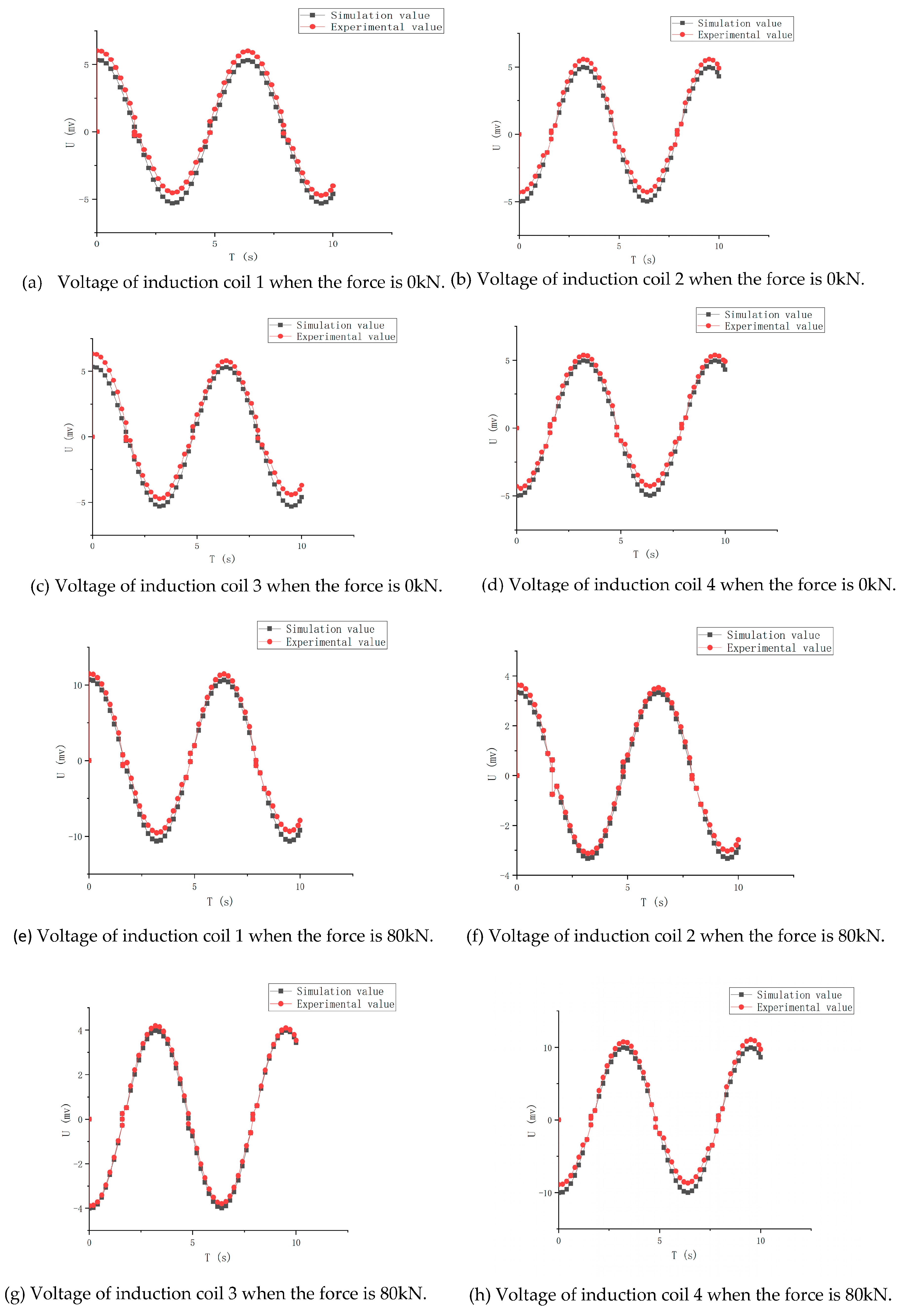
6. Sensor Simulation and Experimental Analysis

The system simulation model of the piezomagnetic sensor is established by using MATLAB/Simulink module, a sinusoidal current is used as the excitation signal in the simulation, as shown in Figure 12. The magnetostrictive force sensor test platform is shown in Figure 13. The platform is composed of the designed piezomagnetic sensor, Hall element, controllable DC power supply, controllable sinusoidal AC power supply, oscilloscope, pressure application device, data acquisition device, and computer. In order to simulate the axial pressure on the iron-cobalt alloy prism under actual working conditions, the pressure regulating device adopts a vertical pressure test platform to apply a force of 0–128 kN to the magnetic sensor along the axis of the excitation magnetic core in the horizontal and vertical directions through the pressurizing device. Different bias magnetic fields are generated by changing the current in the excitation coil through a controllable DC power supply. The magnetic flux and magnetic field strength on the excitation core are measured by the Hall element. An oscillograph is used to measure the waveform of output voltage when the sensor is under force. Each point shall be measured twice and the average value shall be taken to ensure the reliability of the experimental data.

Sinusoidal AC power supply is used in simulation and experiment, which can better compare and observe the change law of each output coil. Therefore, the sinusoidal AC power supply is used to test the difference between the simulated value and the calculated value of the sensor, as shown in Figure 14. When the external force is zero, the voltage of each induction coil presents a periodic distribution, and the voltages of induction coils 1 and 3 are the same, and the voltages of induction coils 2 and 4 are the same. This is because the net magnetic flux generated by the excitation pole in the horizontal direction on each induction coil satisfies Equation (12), that is, zero, so the voltage of each induction coil caused by the excitation magnetic field in the horizontal direction satisfies Equation (13), that is, zero. The net magnetic flux generated by the vertical excitation pole on each induction coil meets Equation (18), that is, it is not zero so the voltage of each induction coil changes under the action of the magnetic field generated by the vertical excitation pole. Therefore, after the superposition of the horizontal and vertical directions, the voltage of each induction coil presents the same change as Equation (22), that is, the voltage of induction coils 1 and 3 is the same, and the voltage of induction coils 2 and 4 is the same. When the external force is not 0, the net magnetic flux generated by each induction coil meets Equation (28). After superposition in the horizontal and vertical directions, the voltage of each induction coil presents the same change as Equation (29), and the total output voltage of the sensor meets Equation (31) and Figure 14. The results show that the derivation of the magnetic circuit of the piezoelectric magnetic sensor is correct.

After the DC power supply is connected, the relationship between the sensor output voltage and force under different bias magnetic fields is tested by changing the current to change the bias magnetic field, as shown in Figure 15. The sensor sensitivity is obtained by deriving the points in Figure 15. When the bias magnetic field is 1.23 kA/m and 84.56 kA/m, the change rate of voltage is small and the sensitivity is small. It can be seen from Figure 15 that when the magnetic field is 1.23 kA/m and 84.56 kA/m, the piezomagnetic coefficient of the iron-cobalt alloy is low, resulting in a small change rate of voltage. Experiments show that under the bias magnetic field of 14.74 kA/m, the piezomagnetic coefficient is the largest and the maximum sensitivity is 0.4394 mV/kN, which is consistent with the simulation results of iron-cobalt alloy in Section 2.

When the bias magnetic field is 14.74 kA/m, there is a good linear relationship between output voltage and force. When the test force is within 0–80 kN, the developed sensor has high sensitivity and good linearity. When the test force is within 80–120 kN, the sensitivity of the sensor decreases slightly, but the reduction speed is slow, which proves that the sensor has no obvious saturation phenomenon. The results verify the correctness of the simulation and magnetic circuit derivation. The calculated values are basically consistent with the simulation, indicating that the output voltage of the sensor can be calculated by Equation (30).

7. Conclusions

Based on the nonlinear piezomagnetic equation, the cylindrical iron-cobalt alloy material is modeled and simulated by using ANSYS finite element simulation software, and the effects of bias magnetic field and stress on the piezomagnetic coefficient are studied. Referring to the working conditions of the tractor force sensor, a new type of piezomagnetic sensor is designed and manufactured. Using the electromagnetic theory and piezomagnetic effect, the three-dimensional model of the magnetic structure and the mathematical model of the magnetic circuit of the sensor are established, and the working principle of the sensor is expounded. The feasibility of the theory is verified by simulation and experiment. According to the simulation and experimental results, when the bias magnetic field intensity is 14.74 kA/m, the piezomagnetic coefficient reaches the maximum value of 9.2 T/GPa. The force measuring range of the sensor is 0–120 kN, the force has high test sensitivity in the range of 0–80 kN, and the test sensitivity of the force in the range of 80–120 kN is slightly low. The sensor has the advantages of simple structure and high sensitivity. It can meet the requirements of accurate force sensing and better adapt to the harsh working environment.

References

1. Ren, W.B. Annealing Process of Precise Control Magnetic Properties of Permalloy. Heat Treat. Met. 2004, 29, 68. [Google Scholar]
2. Ohnuma, I.; Enoki, H.; Ikeda, O.; Kainuma, R.; Ohtani, H.; Sundman, B.; Ishida, K. Phase equilibria in the Fe–Co binary system. Acta Mater. 2002, 50, 379–393. [Google Scholar] [CrossRef]
3. Zhu, Q.; Li, L.; Masteller, M.S.; Del Corso, G.J. An increase of structural order parameter in Fe–Co–V soft magnetic alloy after thermal aging. Appl. Phys. Lett. 1996, 69, 3917. [Google Scholar] [CrossRef]
4. Duck, H.A.; Zhang, D.Z.; Liang, D.; Luzin, V.; Cammarata, R.C.; Leheny, R.L.; Chien, C.L.; Weihs, T.P. Temperature dependent mechanical properties of ultra-fine grained FeCo–2V. Acta Mater. 2003, 51, 4083. [Google Scholar]
5. Dai, W.M.; Yin, H.; Ye, M.J. Fractal Structure of the Core Loss Spectrum of Fe-Co-V Soft Magnetic Alloy. J. Mater. Sci. Eng. 1996, 69, 50–53. [Google Scholar]
6. Lafford, T.A.; Gibbs, M.R.J.; Zuberek, R.; Shearwood, C. Magnetostriction and magnetic properties of iron-cobalt alloys multilayered with silver. J. Appl. Phys. 1994, 76, 6534–6536. [Google Scholar] [CrossRef]
7. Marco, C.; Filoppo, B.; Fumio, N. Fracture Behavior of Cracked Giant Magnetostrictive Materials in Three-Point Bending under Magnetic Fields: Strain Energy Density Criterion. Adv. Eng. Mater. 2016, 18, 2063–2069. [Google Scholar]
8. Wohlfarth, E.P. Ferromagnetic Materials: A Handbook of Properties of Magnetically Ordered Matter; Publishing House of Electronics Industry: Beijing, China, 1993; pp. 122–130. [Google Scholar]
9. Xie, X.L.; Wang, B.W.; Zhou, L.L.; Weng, L.; Sun, Y. Research on torsional ultrasonic attenuation characteristics of the magnetostrictive displacement sensor waveguide. Trans. China Electrotech. Soc. 2018, 33, 689–696. [Google Scholar]
10. Tayalia, P.; Heider, D.; Gillespie, J.J.W. Characterization and theoretical modeling of magnetostrictive strainsensors. Sens. Actuators A Phys. 2004, 1, 267–274. [Google Scholar] [CrossRef]
11. Chang, H.C.; Liao, S.C.; Hsieh, H.S.; Wen, J.H.; Lai, C.H.; Fang, W. Magnetostrictive type inductive sensing pressure sensor. Sens. Actuators A Phys. 2016, 238, 25–36. [Google Scholar] [CrossRef]
12. Atulasimha, J.; Flatau, A.B.; Chopra, I.; Kellogg, R.A. Effect of stoichiometry on sensing behavior of iron-gallium. Proc. SPIE-Int. Soc. Opt. Eng. 2004, 5387, 487–497. [Google Scholar]
13. Yoo, J.H.; Jones, N.J. A performance prediction for Fe Ga magnetostrictive strain sensor using simplified model. IEEE Trans. Magn. 2017, 53, 1–4. [Google Scholar] [CrossRef]
14. Tong, J.; Jia, Y.; Zhang, W. Study on SAW Current Sensor Based on Magnetostrictive Effect. Piezoelectrics Acoustooptics 2017, 39, 662–706. [Google Scholar]
15. Yang, C.H.; Wen, Y.M.; Li, P.; Bian, L.-X. Influence of bias magnetic field on magnetoelectric effect of magnetostrictive/elastic/piezoelectric. laminated composite. Acta Phys. Sin. 2008, 57, 7292–7297. [Google Scholar] [CrossRef]
16. Downey, P.R. Characterization of Bending Magnetostriction in Iron-Gallium Alloys for Nanowire Sensor Applications. Ph.D. Thesis, University of Maryland, College Park, MD, USA, 2008; pp. 4649–4661. [Google Scholar]
17. Cui, X.X.; Whang, B.W.; Li, M.M. Analysis of Output Characteristics and Influencing Factors of Magnetostrictive Force Sensor. Chin. J. Sens. Actuators 2019, 32, 1624–1628. [Google Scholar]
18. Zhao, X.; Luo, X.W.; Wells, L.G. Development of continuous measurement system for soil resistance. Trans. Chin. Soc. Agric. Eng. 2009, 25, 67–71. [Google Scholar]
19. Xu, C.L.; Li, L.H.; Zhao, D.Y.; Li, X.; Li, M.; Zhang, W. Field real-time testing system for measuring work dynamic parameters of suspension agricultural implement. Trans. Chin. Soc. Agric. Mach. 2013, 44, 83–88. [Google Scholar]
20. Feng, J.X.; Zhao, X.; Ma, J.J. Advance on measurement of soil mechanical resistance. Agric. Eng. 2013, 3, 1–4. [Google Scholar]
21. Liu, H.F.; Jia, Z.Y.; Wang, F.J.; Ge, C.-Y. Giant magnetostrictive force sensor and its experimental study. J. Dalian Univ. Technol. 2011, 51, 832–836. [Google Scholar]
22. Han, J.Y.; Gao, X. Development of a shaft type sensor for measuring tractor pull force. Agric. Equip. Veh. Eng. 2014, 52, 10–13. [Google Scholar]
23. Fan, C.Z.; Yang, Q.X.; Yang, W.R.; Yan, R.-g.; Sun, J.-f.; Liu, F.-g. Gian tmagnetostritive force sensor based on inverse magnetostritive effect. Instrum. Tech. Sens. 2007, 4, 5–7. [Google Scholar]
24. Shi, Y.P.; Ni, L.X.; Zhou, Q.G. Study on a new electromagnetic film pressure sensor based on the magnetoelasticity effect. Chin. J. Sens. Actuators 2010, 23, 1256–1260. [Google Scholar]
25. Yu, W.H.; Tian, H.; Liang, C.; Li, C.; Zhao, Y. Soil compactness measuring method based on acceleration compensation and sensor design. Trans. Chin. Soc. Agric. Mach. 2017, 48, 50–256. [Google Scholar]
26. Zhao, D.; Xiao, J.X.; Liu, Y. Overview of smart sensor technology. Transducer Microsyst. Technol. 2014, 33, 4–7. [Google Scholar]
27. Zheng, X.J.; Liu, X.E. A nonlinear constitutive model for Terfenol-D rods. J. Appl. Phys. 2005, 97, 61. [Google Scholar] [CrossRef]
28. Wang, B.W. Preparation of Giant Magnetostrictive Materials and Device Design; Metallurgical Industry Press: Beijing, China, 2003; pp. 68–100. [Google Scholar]
29. Electronic and Hydraulic Hitch Control. Available online: www.boschrexroth.com (accessed on 30 May 2020).
Figure 1. Magnetic domain distribution in iron-cobalt cylinder without force and under force. (a) Magnetic domain without force. (b) Magnetic domain under force.
Processes 10 01218 g001
Figure 2. Magnetic force model of iron-cobalt alloy prism.
Processes 10 01218 g002
Figure 3. Magnetic field distribution in x-z plane of iron-cobalt alloy prism.
Processes 10 01218 g003
Figure 4. Relationship between magnetic induction intensity and compressive stress under different bias magnetic fields.
Processes 10 01218 g004
Figure 5. Relationship between piezomagnetic coefficient and compressive stress under different bias magnetic fields.
Processes 10 01218 g005
Figure 6. Relationship between piezomagnetic coefficient and bias magnetic field under different compressive stress.
Processes 10 01218 g006
Figure 7. Variation diagram of magnetic domain under different magnetic induction intensity. (a) 105.35 kA/m. (b) 14.74 kA/m.
Processes 10 01218 g007
Figure 8. Assembly and stress diagram of piezomagnetic sensor. (a) Stress area diagram of sleeve, (b) Force diagram of sensor.
Processes 10 01218 g008
Figure 9. Structure diagram of piezomagnetic sensor. 1. Vertical excitation core I; 2. Vertical excitation core II; 3. Horizontal excitation core I; 4. Horizontal excitation core II; 5. Induction core 1; 6. Induction core 3; 7. Induction core 4; 8. Induction core 2; 9, 10, 11, 12. Excitation coil; 13, 16, 14, 15. Induction coil1, 2, 3, 4.
Processes 10 01218 g009
Figure 10. Schematic diagram of magnetic circuit.
Processes 10 01218 g010
Figure 11. Schematic diagram of overall magnetic circuit under force.
Processes 10 01218 g011
Figure 12. Sensor system simulation model.
Processes 10 01218 g012
Figure 13. Sensor test platform.
Processes 10 01218 g013
Figure 14. Voltage of each induction coil of piezoelectric magnetic sensor under different external forces. (a) Voltage of induction coil 1 when the force is 0 kN, (b) Voltage of induction coil 2 when the force is 0 kN, (c) Voltage of induction coil 3 when the force is 0 kN, (d) Voltage of induction coil 4 when the force is 0 kN, (e) Voltage of induction coil 1 when the force is 80 kN, (f) Voltage of induction coil 2 when the force is 80 kN, (g) Voltage of induction coil 3 when the force is 80 kN, (h) Voltage of induction coil 4 when the force is 80 kN.
Processes 10 01218 g014
Figure 15. Relationship between sensor output voltage and force under different bias magnetic fields.
Processes 10 01218 g015
Publisher’s Note: MDPI stays neutral with regard to jurisdictional claims in published maps and institutional affiliations.