Stochastic Review Inventory Systems with Deteriorating Items; A Steady-State Non-Linear Approach

Abstract

The primary goal of business organization is optimally maximizing their productivity and profit whilst reducing the cost resulting from lost sales and services given to their customers, which can be achieved by exceeding the balance between the demand and supply. Analyzing real-world situations, including integrated queuing-inventory systems, such as $M/M/1$-systems and $M/M/1/\infty$-systems, can help business organizations reach this goal. This research analyzes integrated queuing-inventory systems with lost sales validated under a deterministic and uniformly distributed order size scheme under continuous review. The limited integrated inventory-queuing $M/M/1/N$-1-system was chosen as subject of our interest due to its closeness to reality. Thus, this system with exponentially distributed deteriorating products and random planning time with lost sales was simulated. This research aimed to analyze customers’ sanctification by studying the addition of the deterioration parameter $\gamma$ to the model under consideration. The proposed model’s demand was based on Poisson, wherein service times and lead times are exponentially distributed. We also examined $M/M/1/\infty$ and $M/M/1/N$-1-systems investigated by Shwarz et al. using the proposed method to solve the linear system of equations obtained from the steady-state system balance equations results obtained are compared to those obtained from simulating the Schwarz approach. The analyzed model was tested for different values of Q, demand rate $\lambda$, and $\gamma$. The obtained results showed a strong dependency between $\gamma$, Q, and $\lambda$, providing the needed information for decision-makers to reach their goals depending on the performance measure of interest.

1. Introduction

Understanding and evaluating the dynamic relationships between demand and supply in a supply chain are the most critical aspects of optimizing a company’s efficiency and profitability [1]. The main goal of every business organization is to balance the demand and supply to reduce the organizational costs produced from lost sales or services given to their customers. It was proven that the inventory control is cost-effective when identifying the trade-off between demand and supply. Inventory control has received much attention in the previous literature as its importance arises from maintaining an accurate inventory level that decreases the cost for every organization [2]. Devising frameworks to reduce the inventory cost and satisfy the customers’ needs is a problem often faced by organizations. Efficient and reliable mathematical models are significant in guaranteeing the success of any inventory management.

Most material resources management systems (MRM) simultaneously possess properties of waiting for line systems and inventory management systems. Their service channel is linked to a system stock, and a level of resources in stock decreases just as the customer service is being completed, which is why these factors should be considered for studying such systems.

Dealing with inventory management systems can be difficult because they involve many interconnected components that are all different in structure [3]. These interacting components are represented as a supply chain network through upstream and downstream linkages, in which suppliers and the mechanisms for maintaining relationships with them are included in the upstream part of the supply chain. The organizations and processes responsible for selling and supplying goods to final customers are found in the downstream section, which can be described as a network of organizations involved in various processes and activities that generate value as products and services to the end customer [4].

In general, good inventory policy positively or negatively impacts supply chain performance. If inventory policies are not well chosen, companies will be charged high costs. Therefore, many companies want to determine the most appropriate inventory policy. In inventory models, the majority of the literature includes different assumptions such as stochastic demand, reduced lead time, product quality, and deterioration rate [5]. Product predictability is a critical aspect of the inventory policy, with many aspects affecting inventory systems. Moreover, during storage, the quality of the majority of the stored goods will worsen, and their value will decrease or be lost. Therefore, in inventory practice, deterioration should be considered.

The manufacturing terms that are used in this article are based on the [6] definition, in which he distinguished between make-to-order (MTO) and make-to-stock (MTS) strategies for the distribution environment. As an example, the strategies were split into assemble-to-order (ATO) [7], where (MTO) refers to the process of generating orders based on real market demand and then fulfilling those orders for the specific customer who placed the order. (MTS) is the process of designing or manufacturing products in response to expected market demand. The ATO approach combines the MTS and MTO strategies. The ATO approach aims to incorporate both make-to-order and make-to-stock manufacturing, enabling goods to be efficiently delivered to consumers while still allowing them to be customized or altered in specific ways based on customer requests.

This research proposes a new integrated queuing-inventory model with the appropriate mathematical distribution applicable in real-life situations by studying and adding the deterioration parameter on many performance measures. This obtains the solution to the replenishment problem with optimal cost. More specifically, the study investigates queuing-inventory systems with deteriorating items that are more popular and realistic [8,9,10].

The main focus of this research is customer satisfaction to operate the inventory system. Most models deal with the cost to determine the optimal policy. This research informs supply chain managers how much to order based on increasing customer satisfaction with the service, including by reducing the waiting time for the actual possession of their demand under deterioration. The random time deterioration aspect in the model makes it difficult for supply chain managers to determine the replenishment policy to ensure a high level of customer satisfaction. Thus, the supply chain manager starts by setting the minor level of customer satisfaction that the company can tolerate; then, the model provides the performance measure that takes this effect into account and the supply chain manager can then alter the value of the reorder quantity until they reach the desired level. Furthermore, supply chain managers may use the performance measures presented in the proposed model to obtain the best order quantity that makes the average waiting time less than a preset value. From a different angle, we may use the performance measures presented in the model to obtain the best order quantity—the number of customers waiting for their orders in less than a preset value for the average number of customers waiting for their orders to be fulfilled.

Furthermore, a pilot study of an integrated limited queuing-inventory system was investigated and studied after adding an exponentially distributed deterioration parameter. The simulated model is used to study the model’s behavior as a birth-and-death process. Developing a new stochastic model for this integrated model with deteriorating items enables studying the probabilistic behavior of the model by analyzing system performance measures. The obtained results are used to investigate the properties of queuing-inventory models in the real world with deteriorating items using stochastic parameters. Evaluating the resulting queuing-inventory model with deteriorating items using simulation after validation could be used to make a reliable vision of related real-world problems.

The distributions used in modeling and simulating the performance analysis are used to calculate and analyze the performance measurements of relevant systems. Our research in the previous literature revealed that classical performance measures such as queue length and waiting for time influence inventory management and vice versa [11,12]. This answers questions such as how the stock management reacts to the queuing of requests and customers due to integrated services. Appropriate performance descriptions for the proposed mathematical model are used to integrate the interaction of queuing for service and stock control. Furthermore, we introduce new explicit performance measures for service systems with continuously reviewed lost sales, deteriorating items, availability, and inventory service grades to directly optimize costs in an integrated model.

The structure of this article is organized as Section 1 contains an overview of general inventory issues and the research subject of inventory and objectives. Section 2 covered the emergence of inventory-queuing model principles and a brief history of replenishment policies found in the literature. In Section 3, we present the standard assumptions for integrated queuing-inventory systems. In contrast, Section 4 discusses a proposed integrated inventory-queuing system with deterioration parameters and the impact of introducing the new parameter to a restricted queuing-inventory model. Conclusions and future studies are presented in Section 5.

2. Related Work

Recently, as business activities grow, there has been a need to organize these activities to reduce corporate costs; thus, operational research methods have been developed and contributed with new modern information technology. One important branch of operations research is inventory management theory. Inventory management is a significant way of optimizing logistic activities.

2.1. Inventory Models with Deterioration

The theory of inventory management was first introduced in the 1960s. Early examples include [13,14,15,16], in addition to [17] who published the abstracts of papers related to the subject from 1953 to 1965. On the other hand, many papers have been published, indicating that deterioration is the action or process of becoming impaired or inferior in quality, functioning, or condition, as a new parameter under study [18]. As an example, in [19], a production lot size model was developed for an inventory system with deteriorating items. The lot size refers to an item ordered for delivery on a specific date or manufactured in a single production run. This study took into account both the varying and constant rates of deterioration. Since it seems difficult to obtain a simple expression for the output lot size in the case of a varying rate, a numerical approach has been proposed. An approximate term for the production lot size was extracted for the constant rate of the deterioration situation. A numerical illustration was solved to demonstrate the effect of deterioration.

A competitive environment arises from frequent economic changes and the intensive networking of supply chain relationships [20]. The concept of supply chain management first appeared in the mid-1990s [21]. Entering these supply chains by companies has been a routine resulting from the market and conditions of such companies. The latest technologies for quick information and data interchange between customers and suppliers have been considered for developing a new model to reduce organizational costs. According to the literature, aspects of supply management, such as exchanging knowledge, are the driving factors ensuring higher competition in the market and a wider variety of activities in the market for both firms and whole chains, according to researchers such as [22].

Later, two mathematical models were developed for an inventory system by Hollier [23], in which the units are deteriorating at a constant rate, and the demand rate negatively and exponentially decreases. Hollier believed that replenishment orders are placed at similar intervals in the first model, whereas in the second model, replenishment periods are variable, so there is no need to regularly issue replenishment orders. In both cases, optimal replenishment policies are calculated. Hollier demonstrated the theory with a numerical example. According to the presented computational results, the constant replenishment duration strategy contributes to a higher total cost.

Manda [24] also developed an order-level inventory model for declining goods with the standardized rate of production and stock-dependent demand. He found shortages reasonable in his article, and excess demand is backlogged. For further illustration, the results are accompanied by numerical examples. Raafat [18] provided a complete and up-to-date survey of published inventory literature for the deteriorating (decaying) inventory models according to the literature. More precisely, some of his articles that recognize the impact of degradation as a function of inventory level on-hand are discussed. Various models’ essential features, extensions, and generalizations as well as a classification scheme and research ideas for the future are discussed.

In addition, a deterministic inventory model was created in [25] wherein the demand is determined by price and the cost of holding inventories is determined on time. The analysis of the deterioration rate and holding costs, as time depends on time and the demand rate depends on the selling price, is a generic policy for deteriorated products. Methods of maximizing profit functions have been used. There may be scarcity, which refers to the idea that we have finite resources and cannot satisfy infinite demand with a backlog that, for example, refers to a stack of financial documents such as loan applications, that need to be handled by a company’s sales department. It is well known that, according to the profit maximization rule, if a company wants to maximize income, it should select a production level where the marginal cost (MC) equals the marginal revenue (MR) and the marginal cost curve is increasing.

The authors in [26] published a regular review of deterministic inventory models for items that are deteriorating. The exponential demand rate is taken into account. The model they present was developed based on the constant rate of item deterioration due to scarcity and demand being partially retroactive. The objective of their research was to determine the optimum order time by reducing inventory costs. Their model was numerically illustrated and the percentage changes also led to the sensitivity analysis.

2.2. Replenishment Policies

It was noticed in the literature that there are three continuous review replenishment policies considered in many studies, explained as follows: (0, Q)-policy, the optimal replenishment policy, in which a fixed order size Q < ∞ raw items are ordered and replenished whenever the inventory is empty, and order size is restricted only to the inventory capacity; (r, Q)-policy, in which whenever the on-hand inventory falls to r ≥ 0 recorder point, fixed-size Q < ∞ raw items are ordered and replenished. It is assumed that r < Q and the maximum inventory capacity in this policy is considered to be $Q+r$ items, and there is at most one outstanding order. Note that this policy ensures that there is no perpetual shortage when a material is no longer in use, as the resource will become perpetual if it was not already perpetual, and when the material is almost entirely out of use, the resource can become a paleo resource (e.g., resources of arrowhead-grade flint). In the (r, S)-policy, whenever the on-hand inventory falls to the $r\ge$ 0 recorder point, the size of the raw items ordered and replenished is considered to be S < ∞ with at most one outstanding (r < S) order. Many studies discussed further advantages, drawbacks, and examples of these policies. The paper entitled flexible service policies for Markov’s two-class inventory system was published in [27]. Their study looks at flexible service policies for a Markov inventory system (r, Q) with two customer classes, ordinary and priority customers. When the inventory falls to a predetermined safety level r, ordinary customers arrive with a probability of receiving p service. First, they set up the state transition equation of the inventory level and derive the distribution of steady-state probability and the system performance measures used for inventory control. Once it is established, a long-term average cost of inventories and a mixed-integer optimization model are established.

Furthermore, for optimum control policies, they presented an improved genetic algorithm. Finally, they studied optimal stock control policies and sensitivities through numerical experiments. In another paper, ref. [28] derived stationary distributions in explicit product form for various $M/M/1$ systems with continuous review inventory and various inventory management policies and with the loss of sales. They thought that demand was Poisson, and service times and lead times were exponentially distributed. The distributions presented by the respective systems are used to calculate performance measures. The critical outcome is that the limits in the queue-length processes are the same as those for the classic $M/M/1/\infty$-system in the infinite waiting room.

2.3. Integrated Queuing-Inventory Models

In the last decade, considerable attention has been paid to research into integrated distribution inventory systems or service inventory systems. Models of integrated queuing inventory and detailed analysis have only recently started. The standard approach is to define a Markovian system process and then use standard methods for optimizing stock control strategies, which are nearly optimal. Many studies over the previous decade have shown the development of integrated queuing inventory models such as the survey, [10,29]. Ref. [30] was the first study carried out in the queuing inventory. Their research attempted to find a description with a limited inventory of approximate performance for the $M/G/1$ queue.

The authors in [31] examined the queuing inventory systems with arrivals from Poisson, exponentially distributed service times, and a zero lead time in backorders, which is an order for a product or service that cannot be immediately fulfilled due to a supply shortage. According to their research, the optimal regeneration strategy does not position an order when the level is positive; it only places an order when the inventory level drops to zero and the queue duration reaches a threshold value. The first example is when the customer thought they was lost when they reached the full final queue of waiting. In [32], the authors found a monotonic threshold structure in the optimal ordering policy. Their study found queue leveraged and average costs were reduced by an optimal policy in which the order-size Q is known. Their foundation was extended to include an endless waiting room with their previous study and permitted an exponential or Erlang lead time for a recharge. Moreover, in a new extensive article [33], a new model was presented with an optimal refill policy to maximize the system profit assuming that the income was generated through the service. Some of the contributions in this regard are as follows: ref. [30], which has been heuristic in finding model performance measures that integrate the queuing interaction for services and inventory control in a sequence of articles. Berman defined the description of the Markov process for different systems, and his co-authors [31,32,33,34] used the classical optimization methods to find optimal inventory control strategies. The built-in literature models combine single-server queuing and an affiliated inventory. These models assume that the demand, which arrives when the inventory is depleted, is back-ordered. In [31,32,33,34,35], the models presented vary in terms of delivery time, time distribution, size of the waiting space, order size, and reorder policy. The authors in [28] investigated the $M/M/1/\infty$ servers with attached inventory in lost sales. When the customers come into a situation where the inventory is depleted, the lost sales regime loses them. It was shown that stationary distribution is a product form in the case of exponentially distributed replenishment lead time for various inventory management policies.

Moreover, it is shown in [28] that a server with an attached inventory can be integrated into standard separable networks if no customers are allowed to join this server’s queue while the inventory is empty. The equilibrium probabilities for these systems were analytically calculated, with explicit formulas for the equilibrium and asymptotic average costs and revenues given. The authors in [31] assumed exponentially distributed interarrival and service times and zero replenishment lead time. The optimal policy for a given order size Q is to position an order when the inventory is empty, and the queue length reaches a particular threshold value. One can expect that an order should already be placed in the case of random lead times if some items are still in stock. This is made precise in [32] for exponential replenishment lead times. The optimal policy for prescribed order size Q is to place an order when the queue length exceeds some threshold value given the inventory level.

Recently, [36] presented a paper about the integration of the corporate inventory under continuous demand. His study depends on queuing theory and inventory theory to analyze enterprise goods’ production rate, the production cycle and shipping rates. Moreover, he constructed an integration model on the corporate inventory under continuous demand; on this basis, he considered and used the AnyLogic simulation platform to analyze the integration model. The simulation results showed that AnyLogic is essential for integrating enterprise inventory resources.

3. Material and Methods

3.1. Queuing Inventory Models

Inventory theory’s lost sales and the queuing theory’s lost customers are technical words for related if not identical incidents in natural systems. The investigators’ fine model selection determines the difference: whether stressing inventory management or emphasizing the service structure, all cases largely ignore the alternative aspect. As previously mentioned, models that integrate both aspects, namely customer queuing and inventory management, are available.

Closed-form solutions are uncommon in the literature. Furthermore, the field of continuous review inventory structures with lost sales are mainly unexplored; Mohebbi and Posner reviewed the literature on lost sales models in their article [37].

In this section, the problem under investigation is an $M/M/1$ queuing system with a service system, attached inventory under constant scrutiny, and missed sales. Detailed performance metrics for service systems with an attached inventory under constant evaluation and missed revenue were also included. In addition, availability metrics, service grades, and inventory performance measures were provided to explicitly allow cost optimization in an integrated model. In this issue of interest, the queuing system has a single service queue with a single server, and single queue customers arrive in a random process at a fixed time. With an attached inventory, single server queuing systems of the $M/M/1$ form are examined.

Each served customer requires precisely one item from the inventory and a random time to complete their service. As a result, if there are no customers in line, the inventory demand rate is equal to the arrival rate of customers; otherwise, the demand rate is equal to the service rate. The vector replenishment lead time—or the time between ordering materials and receiving items—is randomly distributed.

An ongoing inventory review system is characterized as one in which the inventory status is inspected following every application event and orders are placed when the inventory is available. Stock which is physically on the shelf is known as on-hand stock. The systems under examination vary in the scale of refill orders and the reorganization procedure. Clients are not permitted to enter the queue as long as the stock is empty in any scheme. This is similar to the lost income scenario of inventory management. However, when the inventory is available, clients are still allowed to enter a waiting room even if the inventory in the system exceeds the number of customers available.

3.1.1. Problem Assumptions

It was assumed that customers are of stochastically identical behavior. There is a Poisson-$\lambda$-arrival stream to the server, $\lambda >0$. Customers request an amount of service time that is exponentially distributed with a rate of service $\mu >0$. Service times and interarrival times constitute an independent family of random variables.

A replenishment order is instantaneously triggered if the inventory is depleted after a customer’s service is completed. The decision of the order size may be randomized according to a discrete probability density function p on integers $1,2,\dots ,M$, where M is the maximal capacity of the inventory. Thus, the size of a replenishment order is k with probability $p_k$ where ${\sum }_{k=1}^M{p}_k=1$. The corresponding discrete distribution function and its tail distribution function will be denoted by $F_p$ and $\overline{F_p}:=1-F_p$, respectively. We abbreviate the probability that the size of a replenishment order is at least k units by $q_k$, i.e., $q_k=\overline{F_p}={\sum }_{h=k}^M{p}_h$. The mean order size is $\overline{p}={\sum }_{k=1}^{M}k{p}_k$. Fixed (deterministic) order quantities are described using one-point distributions for the order size distribution. The replenishment lead time is exponentially distributed with parameter $\nu >0$. Order size decisions and lead times are independent of the arrival and service times. The manufacturing of products from the distribution system is performed according to customer demand on a make-to-stock ($MTS$) basis, in which customers can purchase and receive items at the same time, allowing for a short response time.

The service to the customer only begins when the inventory is not depleted, and that service is given to the customer at the head of the line by giving them exactly one item. There are two measures to evaluate the system depending on the reaction of customers when the inventory is depleted. The first measure is Customer satisfaction ($Cs$), which is the customers who are already waiting in the queue when the inventory is empty. Note that when the inventory is empty, customers will not be satisfied. The second measure is lost sales, which happens when the inventory is empty, or if the number of customers who are waiting in the queue is greater than the number of items already in the inventory. Furthermore, new customers who reach the system will not enter the system. In general, both measures give us an indication of $Cs$.

The customer satisfaction measures are based on the fact that the customer’s demand is not fulfilled. We suggested indicators for the level of customer satisfaction by computing two rates:

• The first-rate concerns customers who have already entered the system while the inventory is not empty upon their arrival, but the quantity in hand deteriorated during the waiting time and became less than what they requested, making the customer wait longer.
• The second rate concerns the arrival of customers when the inventory is empty. In this case, they will be blocked.

These two quantities combined measure customer satisfaction as a percentage of total arrivals.

This study is based on Berman and Kim [31] who showed that an excellent policy does not place an order in an exponential system of zero lead times unless the inventory is empty and a certain amount of customers are waiting. The set of feasible policies is defined by fixing the reorder point 0 and having random general order sizes only restricted by inventory ability. In this category of practicable policies, using the deterministic order size and explicit definitions of stable status behavior for the (demand/inventory) process, the vectors process for (queue length/inventory sized) is minimized in a strongly stochastic order. That is, the optimal ($r=0,Q$) policy structure in this category is $Q\in \mathbb{N}+$. This observation is the reason behind the $M/M/1$ inventory queue investigation, wherein the feasible policy set is prescribed by the $r\ge 0$ reorder and Q deterministic order.

3.1.2. Mathematical Formulation

We consider the birth–death process, a particular case of continuous-time Markov process where the state transitions are of only two types: “births”, which increase the state variable by one; and “deaths”, which decrease the state one.

The integrated queuing-inventory model with lost sales considered herein is shown in Figure 1. Furthermore, the constructed balance equations depend on the birth-and-death process, wherein rate in = rate out. The steady-state distribution is considered, in which the long-run behavior of Markov chains is considered; as time approaches infinity, a Markov chain may settle down and exhibit steady-state behavior.

From the aforementioned assumptions made regarding the system’s stochastic nature, the attached inventory has M item capacity. The reorder policy is used to evaluate the randomized order policy. Let $X\left(t\right)$ denote the number of customers present at the server at time $t\ge 0$, either waiting or in-service (queue length), and let $Y\left(t\right)$ denote the on-hand inventory at time $t\ge 0$. Then, $Z=\left(\right(X\left(t\right),Y\left(t\right)),t\ge 0)$ is a continuous-time Markov process for the $M/M/1/N-1$- the system with inventory management, reorder point 0, and the random size of replenishment orders. The state-space of Z is $E_{ZN}=(n,k):n\in \{0,1,\dots ,N\},1\le k\le M\cup (n,0):n\in \{0,1,\dots ,N-1\}$, since the inventory can only be depleted after a customer has been served who took the last item from the inventory and no customers join the queue during the replenishment lead time.

The list of variables introduced to build the balance equations and the investigated performance metrics was given in

Table 1. The list of variables introduced during the building of the balance equations and the investigated performance metrics.

Term	Definition
Q	The ordered quantity by the management
µ	The number of customers served per unit time (the service rate)
$\lambda up$	The number demand arrived per unit of time (customers arrival rate)
$p_k$	The probability of the replenishment order with size k
$F_P$	The discrete distribution
$\overline{F_p}$	The tail distribution corresponding to probability p
$q_k$	The probability of the replenishment order is at least k units
$\upsilon$	The average lead intensities/rates
$\gamma$	The average deterioration intensities/rates per unit
$\overline{I}$	The average inventory level
$\overline{p}$	The mean order size of new delivery
$E_Z$	State space of stochastic process representing the current state of the inventory system = {(n,k):n $\in N,k\in \left\{0,\dots \dots ,M\right\}\}$
M	The maximal size of the storage space measured in units of inventory
N	The maximal capacity of the number of customers in the system at any given time
n	The current number of customers in the system
k	The current number unites available in the system
${\lambda }_R$	The mean number of replenishments per time unit
${\lambda }_A$	The mean number of customers arriving per unit time
$\overline{LS}$	The average number of lost sales incurred per unit of time
${\overline{LS}}_c$	The expected number of lost sales per cycle
${\overline{L}}_0$	The mean number of customers in the system

.

The global balance equations are given as:

$$\begin{array}{ccc}\hfill \pi (n,M)(\lambda +\mu (1-{\delta }_{0n}))& =& \pi (n-1,M)\lambda (1-{\delta }_{0n})+\pi (n,0)\nu p_M,\hfill \\ \hfill \pi (n,k)(\lambda +\mu (1-{\delta }_{0n}))& =& \pi (n-1,k)\lambda (1-{\delta }_{0n})+\pi (n+1,k+1)\mu \hfill \\ & +& \pi (n,0)\nu p_k,M>k\ge 1,\hfill \\ \hfill \pi (n,0)\nu & =& \pi (n+1,1)\mu .\hfill \end{array}$$

Let ${\delta }_{ij}$ be an indicator variable that takes the value 1 when (i = j) and takes the value 0 otherwise. Thus, for the queueing systems, the departure rate is $\mu$ if there are customers in the system, which are represented by the indicator (1 $-{\delta }_{0n}$) for all n.

$${\delta }_{ij}=\left\{\begin{array}{c}1if(i=j)\hfill \\ \\ 0ifotherwise\hfill \end{array}\right.$$

(1)

Schwarz et al. in [28] were able to prove the steady-state solution for the global balance equations in Theorem A1, given in Appendix A.

3.1.3. M/M/1/N-System with Inventory and Lost Sales

The critical issue was that a long queue does not mean that new arrivals would be turned away because some goods are still available in the inventory. Customers who arrive when all waiting places are filled are automatically refused, even though there are still items in the inventory, which is a benefit of our previous models to some degree.

Under the $FCFS$ regime, we have a single server with a small number of $N-1$ waiting places. If the number of customers in the system at the time of a customer’s arrival is less than N and the on-hand inventory is positive, the customer is admitted to the system; otherwise, the customer is not admitted. They vanish and are never seen again.

The global balance equations for the $M/M/1/N$-system with inventory and lost sales are given as:

$$\begin{array}{ccc}\hfill \pi (n,k)(\lambda (1-{\delta }_{Nn})+\mu (1-{\delta }_{0n}))& =& \pi (n-1,k)\lambda (1-{\delta }_{0n})+\pi (n+1,k+1)\mu (1-{\delta }_{Nn})\hfill \\ & \times & (1-{\delta }_{kM})\hfill \\ & +& \pi (n,0)\nu p_k(1-{\delta }_{Nn}),0\le n\le N,1\le k\le M,\hfill \\ \hfill \pi (n,0)\nu & =& \pi (n+1,1)\mu ,0\le n\le N-1\hfill \end{array}$$

In terms of steady-state solution for the global balance equations, the ${\delta }_{ij}$ indicator variable is assumed as defined in Equation (1)

In [28], Schwarz et al. were able to prove the steady-state solution for the global balance equations in Theorem A2, given in Appendix A.

3.1.4. Performance Measures

The measures of system performance of the $M/M/1/N-1$-system with inventory are:

$$\overline{I}=\frac{{\mu }^{N+1}-{\lambda }^{N+1}}{{\mu }^{N+1}(\overline{p}+\frac{\lambda }{\nu })-{\lambda }^{N+1}(\overline{p}+\frac{\mu }{\nu })}\sum _{k=1}^{M}k{q}_k,=\frac{{\mu }^{N+1}-{\lambda }^{N+1}}{K_Y\mu ({\mu }^N-{\lambda }^N)}\sum _{k=1}^{M}k{q}_k,$$

(2)

$${\lambda }_R=\frac{({\mu }^N-{\lambda }^N)\lambda \mu }{{\mu }^{N+1}(\overline{p}+\frac{\lambda }{\nu })-{\lambda }^{N+1}(\overline{p}+\frac{\mu }{\nu })},=\frac{\lambda }{K_Y},$$

(3)

$${\lambda }_A=\frac{({\mu }^N-{\lambda }^N)\lambda \mu \overline{p}}{{\mu }^{N+1}(\overline{p}+\frac{\lambda }{\nu })-{\lambda }^{N+1}(\overline{p}+\frac{\mu }{\nu })},=\frac{\lambda \overline{p}}{K_Y},$$

(4)

$$\overline{LS}=\lambda \frac{\lambda }{\nu }{K}_Y^{-1}+\lambda {\left(\frac{\lambda }{\mu }\right)}^N\overline{p}{K}^{-1},$$

(5)

$$\overline{L{S}_c}=\frac{\lambda }{\nu }+{\left(\frac{\lambda }{\mu }\right)}^N\overline{p}{K}_X^{-1},$$

(6)

$$\beta =\frac{({\mu }^N-{\lambda }^N)\mu \overline{p}}{{\mu }^{N+1}(\overline{p}+\frac{\lambda }{\nu })-{\lambda }^{N+1}(\overline{p}+\frac{\mu }{\nu })},=\frac{\overline{p}}{K_Y},$$

(7)

$$\overline{W_0}=\frac{1}{\mu -\lambda }(1+\frac{\lambda }{\nu \overline{p}})-\frac{N{\lambda }^N}{\mu ({\mu }^N-{\lambda }^N)}(1+\frac{\mu }{\nu \overline{p}}),$$

(8)

$$\overline{W}=\frac{\lambda ({\mu }^{N-1}-{\lambda }^{N-1})}{(\mu -\lambda )({\mu }^N-{\lambda }^N)}(1+\frac{\lambda }{\nu \overline{p}})-(N-1)\frac{{\lambda }^N}{\mu ({\mu }^N-{\lambda }^N)}(1+\frac{\mu }{\nu \overline{p}})$$

(9)

In Appendix B, some of the mentioned measures are proven.

The mean number of waiting customers $\overline{L}$ is

$$\begin{array}{ccc}\hfill \overline{L}& =& \overline{L_0}-p(X>0)\hfill \\ & =& \overline{L_0}-(1-K^{-1}(\overline{p}+\frac{\lambda }{\nu }))\hfill \\ & =& \frac{{\lambda }^2({\mu }^{N-1}-{\lambda }^{N-1})}{{\mu }^{N-1}{(\mu -\lambda )}^{2}K}(\overline{p}+\frac{\lambda }{\nu })-\frac{(N-1){\lambda }^{N+1}}{{\mu }^N(\mu -\lambda )K}(\overline{p}+\frac{\mu }{\nu })\hfill \end{array}$$

The customer mean sojourn time $\overline{W_0}$ is

$$\begin{array}{ccc}\hfill \overline{W_0}& =& \frac{{\overline{L}}_0}{{\lambda }_A}=\frac{1}{\mu -\lambda }(1+\frac{\lambda }{\nu \overline{p}})-\frac{N{\lambda }^N}{\mu ({\mu }^N-{\lambda }^N)}(1+\frac{\mu }{\nu \overline{p}})\hfill \end{array}$$

The customer mean waiting time $\overline{W}$ is

$$\begin{array}{ccc}\hfill \overline{W}& =& \frac{\overline{L}}{{\lambda }_A}=\frac{\lambda ({\mu }^{N-1}-{\lambda }^{N-1})}{(\mu -\lambda )({\mu }^N-{\lambda }^N)}(1+\frac{\lambda }{\nu \overline{p}})-\frac{(N-1){\lambda }^N}{\mu ({\mu }^N-{\lambda }^N)}(1+\frac{\mu }{\nu \overline{p}})\hfill \end{array}$$

3.1.5. The Cost Function

We demonstrated the usual cost and reward functions for the required performance measures. The total cost could be found by adding up all the cost functions. The first cost function, ${\lambda }_R\times K$, is the ordering cost associated with replenishment orders that occur with the reorder rate ${\lambda }_R$; the second cost function, $\overline{I}\times h$, represents the holding costs for an inventory of mean size $\overline{I}$; the third cost function, $\overline{LS}\times l$, represents the shortage costs for the mean number of lost sales $\overline{LS}$; the fourth cost function, $\overline{L}\times \omega$, is the waiting costs for the mean number $\overline{L}$ of waiting for customers; and the last cost function, $\overline{V}\times \sigma$, is the costs for the mean number $\overline{V}$ of customers in service. Thus, the total cost can be given as:

$$F={\lambda }_R\times K+\overline{I}\times h+\overline{LS}\times l+\overline{L}\times \omega +\overline{V}\times \sigma .$$

We presented a numerical example illustrating the calculations of performance measures and the total cost in two different order schemes, namely deterministic and uniformly distributed order size.

In a sales company based on the sale of one type of game for children, if the arrival rate of customers to fund officers is 30 customers per hour, the service rate is 35 customers per hour and the lead time rate is 0.1 unit per day. The optimal policy for ordering the type of game is to be determined based on the following data: order size (Q) = 500 units per day; ordering cost (K) = USD 50 per order; holding cost (h) = USD 0.02 per unit per day; shortest cost (l) = USD 2 per day; waiting cost in queue USD 5 per day; P (probability that lost sales case of shortage) = 0.4; waiting cost in system $\omega$ = USD 8 per day; and revenue to the system (R) = USD 2000 per day. Based on the given data, we can obtain the total cost for our distributions that we studied as follows.

For deterministic order size,

$\rho =0.85714286,\overline{L_o}=6,{\lambda }_R=0.048,\overline{I}=200.4,\beta =0.8,\overline{W_o}=0.25,\overline{W}=0.21428571,\overline{LS}=6,\overline{L{S}_c}=125,P(Y=0)=0.2,F=50.98$

For uniform order size,

$\rho =0.85714286,\overline{L_o}=6,{\lambda }_R=0.079,\overline{I}=111.63,\beta =0.67,\overline{W_o}=0.2998,\overline{W}=0.26,\overline{LS}=9.9,\overline{L{S}_c}=125,P(Y=0)=0.333,F=58.77$

3.2. Classical Inventory Queuing System with Deterioration

In this work, it was assumed that products from the distribution system are manufactured according to customer demand on a make-to-stock ($MTS$) basis, whereby customers can simultaneously purchase and receive items, allowing for a short response time. $MTS$ is an example of a “push supply chain” technique. Decisions regarding when and how much to create in a push supply chain strategy are based on expected consumer demand. In $MTS$, production is planned well in advance based on expected demand. Therefore, the use of resources is also planned accordingly to facilitate efficiency. Moreover, the timing and amount of products are planned ahead of time. As a result, work may be scheduled, and the amount of work that remains may be determined at any moment in time, and the finished goods are in the store and ready to be purchased immediately. The customer can purchase a product and have it delivered simultaneously.

The service system with an attached inventory was investigated in this study, wherein indistinguishable consumers arrived one by one and required service. Under the first-come–first-served ($FCFS$) system, there is a single server with an endless waiting room and an inventory with a maximum capacity of M (identical) items. For service, each customer requires precisely one item from the inventory, and the on-hand inventory drops by one when each time service is completed. If the server is ready to serve a customer at the front of the line and there is no inventory item, service will only begin when the next replenishment arrives at the inventory (and then immediately). Customers who arrive while the server is waiting for a replenishment order are refused and are lost to the system (“lost sales”). A served consumer exits the system immediately, and the relevant item is withdrawn from the inventory at the same moment. If there is another customer in line and at least one more item in stock, the next service will begin right away. There is a policy in place that decides whether a replenishment order is placed at each decision point and the number of items requested. Arrival and departure epochs are the only decision epochs that are permitted. It was expected that, at most, one order was constantly outstanding. Customers queuing and inventory storage are both costs associated with system operation.

We have a fixed inventory holding cost h per item and time unit; a fixed replenishment ordering cost K; a shortage cost l per unit of missed sales; a cost per customer and time unit in the waiting room; and a cost per customer and time unit in service. When a customer’s service is complete, the system receives the revenue of R. The number of customers present at the server at time $t\ge 0$ (either waiting or in-service) was marked by $X\left(t\right)$, while the on-hand inventory was designated by $Y\left(t\right)$. $Z=\left(\right(X\left(t\right),Y\left(t\right)),t\ge 0)$ was used to represent the combined queue length and inventory process.

Z’s state space is $E_Z=(n,k):n\in N_0$, $k=0\dots ,M$, where M is the inventory’s maximum size, which is determined by the order policy, stating that if the inventory is exhausted after a customer’s service is completed, a replenishment order is immediately triggered. The order size choice can be randomized using a discrete probability density function p on the integers $1,2,\dots ,M$, where M is the inventory’s maximum capacity. As a result, the size of a replenishment order is k, with a probability of $p_k$, where ${\sum }_{k=1}^M{p}_k=1$.

The main parameter that is added to our limited $M/M/1/N-1$ system is that the deterioration parameter $\gamma$ is exponentially distributed and has a value of less than Q. This parameter can be seen in Figure 2 and it is represented by the red arrow that returns from the state under consideration from the previous state. The parameter follows an exponential distribution with $k\gamma$ rate, where k is the number of items in the system at state ($I,j$), equal to j, so $k\in [1,M]$.

Mathematical Formulation

The average time during which a unit remains available before deterioration is $\frac{1}{\gamma }$. In our study, if one unit deteriorates, it is represented by $1\gamma$; if two units deteriorate, they are represented by $2\gamma$. Furthermore, it follows that if M units deteriorate, they are represented by $M\gamma$.

The new balance equations that describe the system studies are derived as follows, for $i=0$,

$$\begin{array}{ccc}\hfill \nu \pi (0,0)& =& \mu \pi (1,1)+\gamma \pi (0,1)\hfill \\ \hfill \lambda \pi (0,1)+\gamma \pi (0,1)& =& \nu P_1\pi (0,0)+\mu \pi (1,2)+2\gamma \pi (0,2)\hfill \\ \hfill \lambda \pi (0,2)+2\gamma \pi (0,2)& =& \nu P_2\pi (0,0)+\mu \pi (1,3)+3\gamma \pi (0,3)\hfill \end{array}$$

In numerical calculations, first, the maximum system size for the customer (N) is chosen. Different order quantity values are chosen every time a new order is placed (Q). Different values of the average arrival rate of customers ($\lambda$) are chosen. The average lead time (time needed to deliver the new order quantity) ($\nu$) is chosen. The average service rate (number of customers served per unit of time) ($\mu$) is chosen. The distribution of the quantity delivered (P) is chosen. The deterioration parameter $\gamma$ is less than the order quantity Q. Then, the coefficient matrix (A) with dimensions ($N+1\times Q+1$) is then generated using MATLAB with the aforementioned parameters. After that, the probability matrix ($\pi (n,k)$) is calculated by multiplying the inverse of the coefficient matrix (A) by a vector with a length ($N+1$).

The expected time until deuteriation for any unit in stock is assumed to be exponentially distributed with a mean of $\frac{1}{\gamma }$. This is true for any unit in the inventory independent of each other. Therefore, each unit in the inventory is subject to deteriorate independently from the other units. The physical meaning is that the deterioration rate should not exceed the order quantity to exclude the possibility that the new order deteriorated completely before it arrived at the market to make the assumptions more realistic.

The probability matrix ($\pi (n,k)$) is used to generate the marginal probabilities (X) and (Y). Moreover, it is used to calculate performance measures.

4. Results and Discussion

4.1. Numerical Analysis

A numerical analysis was performed to illustrate the results of simulating the system of a limited number of $N-1$ waiting places such that only N customers are admitted to the system simultaneously with fixed-order quantity Q.

We compare the proposed framework on the performance measures at specific values of fixed-order quantity Q, the average rate of arrival customers $\lambda$, the service rate $\mu$, and the time required to deliver the new order quantity $\nu$, where it is assumed to be a case wherein the order quantity is fixed and the delivery is fixed.

4.1.1. The Effect of $\lambda$ on Performance Measures for Different Q Values

In the following

Table 2. The effect of $\lambda$ on performance measures at Q = 15.

Q	$\mathit{\lambda }$	$\overline{\mathit{I}}$	${\mathit{\lambda }}_{\mathit{R}}$	${\mathit{\lambda }}_{\mathit{A}}$	$\overline{{\mathit{L}}_{\mathit{S}}}$	${\overline{\mathit{L}\mathit{S}}}_{\mathit{c}}$	$\mathit{\beta }$	$\overline{{\mathit{L}}_{\mathit{o}}}$	$\overline{\mathit{L}}$	$\overline{{\mathit{W}}_{\mathit{o}}}$	$\overline{\mathit{W}}$	F
15	11	3.6886	0.943	7.543	3.457	3.667	0.686	0.324	0.079	0.043	0.010	8.532
15	15	3.487	1.154	9.231	5.769	5.000	0.615	0.500	0.167	0.054	0.018	10.782
15	25	2.776	1.531	12.245	12.755	8.333	0.490	1.250	0.694	0.102	0.057	18.028
15	40	2.126	1.874	14.994	25.006	13.341	0.375	7.649	6.761	0.510	0.451	36.101

,

Table 3. The effect of $\lambda$ on performance measures at Q = 25.

Q	$\mathit{\lambda }$	$\overline{\mathit{I}}$	${\mathit{\lambda }}_{\mathit{R}}$	${\mathit{\lambda }}_{\mathit{A}}$	$\overline{{\mathit{L}}_{\mathit{S}}}$	${\overline{\mathit{L}\mathit{S}}}_{\mathit{c}}$	$\mathit{\beta }$	$\overline{{\mathit{L}}_{\mathit{o}}}$	$\overline{\mathit{L}}$	$\overline{{\mathit{W}}_{\mathit{o}}}$	$\overline{\mathit{W}}$	F
25	11	7.020	0.660	8.850	2.420	3.667	0.780	0.324	0.079	0.038	0.009	10.370
25	15	6.500	0.833	10.833	4.167	5.000	0.722	0.500	0.167	0.046	0.015	11.907
25	25	5.484	1.172	15.234	9.776	8.333	0.609	1.250	0.694	0.082	0.046	17.455
25	40	4.445	1.518	19.737	20.263	13.346	0.493	7.653	6.765	0.388	0.343	33.430

,

Table 4. The effect of $\lambda$ on performance measures at Q = 33.

Q	$\mathit{\lambda }$	$\overline{\mathit{I}}$	${\mathit{\lambda }}_{\mathit{R}}$	${\mathit{\lambda }}_{\mathit{A}}$	$\overline{{\mathit{L}}_{\mathit{S}}}$	${\overline{\mathit{L}\mathit{S}}}_{\mathit{c}}$	$\mathit{\beta }$	$\overline{{\mathit{L}}_{\mathit{o}}}$	$\overline{\mathit{L}}$	$\overline{{\mathit{W}}_{\mathit{o}}}$	$\overline{\mathit{W}}$	F
33	11	9.597	0.532	9.048	1.952	3.667	0.823	0.324	0.079	0.036	0.009	12.361
33	15	9.015	0.682	11.951	3.409	5.000	0.773	0.500	0.167	0.043	0.014	13.530
33	25	7.829	0.987	16.776	8.224	8.333	0.609	1.250	0.694	0.075	0.041	18.107
33	40	6.541	1.318	22.405	17.595	13.350	0.560	7.655	6.767	0.342	0.302	32.720

and

Table 5. The effect of $\lambda$ on performance measures at Q = 50.

Q	$\mathit{\lambda }$	$\overline{\mathit{I}}$	${\mathit{\lambda }}_{\mathit{R}}$	${\mathit{\lambda }}_{\mathit{A}}$	$\overline{{\mathit{L}}_{\mathit{S}}}$	${\overline{\mathit{L}\mathit{S}}}_{\mathit{c}}$	$\mathit{\beta }$	$\overline{{\mathit{L}}_{\mathit{o}}}$	$\overline{\mathit{L}}$	$\overline{{\mathit{W}}_{\mathit{o}}}$	$\overline{\mathit{W}}$	F
50	11	15.154	0.377	9.617	1.383	3.667	0.874	0.324	0.079	0.034	0.008	17.207
50	15	14.492	0.492	12.541	2.459	5.000	0.836	0.500	0.167	0.040	0.013	17.888
50	25	13.064	0.739	18.842	6.158	8.333	0.754	1.250	0.694	0.066	0.037	21.074
50	40	11.386	1.029	26.249	13.751	13.359	0.656	7.658	6.770	0.292	0.258	33.520

, Q = 15, 25, 33 and 50. $\lambda$ = 11, 15, 25 and 40. The fixation of $\mu$ = 45, $\nu$ = 3, and the size of the system to accommodate the customers N = 40. It was noticed that the average stock level $\overline{I}$ decreases as it increases $\lambda$ for each Q. For ${\lambda }_R$, it was noticed that it increases as $\lambda$ increases because it measures the rate of reordering per unit of time and for ${\lambda }_A$, which is the rate of arrival of customers for each time unit that increases with an increase $\lambda$. The average number of lost sales and the average number of lost sales in each order cycle ($\overline{LS}$, ${\overline{LS}}_c$) increase with the increase in the flow rate. The service level $\beta$ also decreases by increasing $\lambda$. The average number of customers in the whole system and the average number of customers in a queue increase ($\overline{L}$, $\overline{L_0}$) with increasing $\lambda$. The average customer waiting time and average stay increase ($\overline{W}$, $\overline{W_0}$) with the increase in the arrival rate and the cost F increases.

4.1.2. The Effect of $\mu$ on Performance Measures for Different Q Values

In the following

Table 6. The effect of $\mu$ on performance measures at Q = 15.

Q	$\mathit{\lambda }$	$\overline{\mathit{I}}$	${\mathit{\lambda }}_{\mathit{R}}$	${\mathit{\lambda }}_{\mathit{A}}$	$\overline{{\mathit{L}}_{\mathit{S}}}$	${\overline{\mathit{L}\mathit{S}}}_{\mathit{c}}$	$\mathit{\beta }$	$\overline{{\mathit{L}}_{\mathit{o}}}$	$\overline{\mathit{L}}$	$\overline{{\mathit{W}}_{\mathit{o}}}$	$\overline{\mathit{W}}$	F
15	10	4.126	0.816	6.524	2.476	3.035	0.728	6.444	5.548	0.988	0.850	13.617
15	16	4.121	0.818	6.545	2.455	3.000	0.727	4.745	4.182	0.725	0.639	11.985
15	20	4.121	0.818	6.545	2.455	3.000	0.727	4.617	4.167	0.705	0.637	11.888
15	35	4.121	0.818	6.545	2.455	3.000	0.727	4.488	4.231	0.686	0.646	11.812

,

Table 7. The effect of $\mu$ on performance measures at Q = 25.

Q	$\mathit{\lambda }$	$\overline{\mathit{I}}$	${\mathit{\lambda }}_{\mathit{R}}$	${\mathit{\lambda }}_{\mathit{A}}$	$\overline{{\mathit{L}}_{\mathit{S}}}$	${\overline{\mathit{L}\mathit{S}}}_{\mathit{c}}$	$\mathit{\beta }$	$\overline{{\mathit{L}}_{\mathit{o}}}$	$\overline{\mathit{L}}$	$\overline{{\mathit{W}}_{\mathit{o}}}$	$\overline{\mathit{W}}$	F
25	10	7.319	0.560	7.286	1.714	3.058	0.813	8.911	8.015	1.223	1.100	18.337
25	16	7.313	0.562	7.312	1.688	3.000	0.813	7.741	7.179	1.059	0.982	17.198
25	20	7.313	0.562	7.312	1.688	3.000	0.813	7.653	7.203	1.047	0.985	17.132
25	35	7.313	0.563	7.313	1.688	3.000	0.813	7.565	7.308	1.035	0.999	17.079

,

Table 8. The effect of $\mu$ on performance measures at Q = 33.

Q	$\mathit{\lambda }$	$\overline{\mathit{I}}$	${\mathit{\lambda }}_{\mathit{R}}$	${\mathit{\lambda }}_{\mathit{A}}$	$\overline{{\mathit{L}}_{\mathit{S}}}$	${\overline{\mathit{L}\mathit{S}}}_{\mathit{c}}$	$\mathit{\beta }$	$\overline{{\mathit{L}}_{\mathit{o}}}$	$\overline{\mathit{L}}$	$\overline{{\mathit{W}}_{\mathit{o}}}$	$\overline{\mathit{W}}$	F
33	10	9.923	0.448	7.621	1.379	3.075	0.851	11.197	10.301	1.496	1.352	22.813
33	16	9.917	0.450	7.650	1.350	3.000	0.850	10.260	9.697	1.341	1.268	21.892
33	20	9.917	0.450	7.650	1.350	3.000	0.850	10.189	9.739	1.332	1.273	21.839
33	35	9.917	0.450	7.650	1.350	3.000	0.850	10.119	9.861	1.323	1.289	21.797

and

Table 9. The effect of $\mu$ on performance measures at Q = 50.

Q	$\mathit{\lambda }$	$\overline{\mathit{I}}$	${\mathit{\lambda }}_{\mathit{R}}$	${\mathit{\lambda }}_{\mathit{A}}$	$\overline{{\mathit{L}}_{\mathit{S}}}$	${\overline{\mathit{L}\mathit{S}}}_{\mathit{c}}$	$\mathit{\beta }$	$\overline{{\mathit{L}}_{\mathit{o}}}$	$\overline{\mathit{L}}$	$\overline{{\mathit{W}}_{\mathit{o}}}$	$\overline{\mathit{W}}$	F
50	10	15.516	0.315	8.021	0.979	3.311	0.895	16.410	15.514	2.046	1.934	33.125
50	16	15.509	0.316	8.053	0.979	3.000	0.895	15.749	15.187	1.956	1.886	32.462
50	20	15.509	0.316	8.053	0.979	3.000	0.895	15.700	15.250	1.950	1.894	32.425
50	35	15.509	0.316	8.053	0.979	3.000	0.895	15.650	15.393	1.944	1.912	32.395

, it was assumed in this case that Q = 15, 25, 33 and 50. $\mu$ = 10, 16, 20 and 35. The fixation of $\lambda$ = 9, $\nu$ = 3 and the size of the system to accommodate the customers N = 40. It was noticed that the average stock level $\overline{I}$ decreases as it increases $\mu$ for each Q. For ${\lambda }_R$, it was noticed that it increases as $\mu$ increases because it measures the rate of reordering per unit of time and for ${\lambda }_A$, which is the rate of arrival of customers for each time unit that increases with an increase $\mu$. The average number of lost sales and the average number of lost sales in each order cycle ($\overline{LS}$, ${\overline{LS}}_c$) increase with the increase in the flow rate. The service level $\beta$ also decreases by increasing $\mu$. The average number of customers in the whole system and the average number of customers in a queue increase ($\overline{L}$, $\overline{L_0}$) with increasing $\mu$. The average customer waiting time and average customer length of stay increase ($\overline{W}$, $\overline{W_0}$) with the increase in the service rate. Moreover, the cost F decreases. It can be observed that after $\mu$ = 16, $\overline{I}$, ${\lambda }_R$, ${\lambda }_A$, $\overline{LS}$, ${\overline{LS}}_c$ and $\beta$ seem to be constant.

In order to check the effect of $\nu$ on performance measures for different Q values, it was assumed that Q = 15, 25, 33 and 50. $\nu$ = 3, 10, 25 and 40. Fixation of $\lambda$ = 14, $\mu$ = 15, and the size of the system to accommodate the customers N = 40. It was noticed that the average stock level $\overline{I}$ decreases as it increases $\nu$ for each Q. For ${\lambda }_R$, it was noticed that it increases as $\nu$ increases because it measures the rate of reordering per unit of time and for ${\lambda }_A$, which is the rate of arrival of customers for each time unit that increases with an increase $\nu$. Moreover, the average number of lost sales and the average number of lost sales in each order cycle ($\overline{LS}$, ${\overline{LS}}_c$) increase with the increase in flow rate. The service level $\beta$ also decreases by increasing $\nu$. The average number of customers in the whole system and the average number of customers in a queue increase ($\overline{L}$, $\overline{L_0}$) with increasing $\nu$. The average customer waiting time and the average stay of the customer increase ($\overline{W}$, $\overline{W_0}$) with the increase in the lead time and the cost F decreases. In general, there are some measures that change their behavior depending on Q values, such as ($\overline{L}$, $\overline{L_0}$, and F); for example, when $Q=15$ and $Q=25$, these measures decrease, while for $Q=33$ and $Q=50$, they increase.

4.2. M/M/1/N-System with Deterioration under Deterministic and Uniformly Distributed Order Size

In this section, the results were obtained from simulating a MATLAB program designed to model a limited inventory system with lost sales and a deterioration parameter under deterministic order size probabilities. The maximum system size for the customer (N) is chosen to be equal to 10. Every time a new order is placed (Q), the order quantity is chosen to have different values from the range of 5–35 with step 5. The average arrival rate of customers ($\lambda$) was chosen to have different values from the range 5–35 with step 5. The average lead time (time needed to deliver the new order quantity) ($\nu$) was chosen to be equal to 1. The average service rate (number of customers served per unit of time) ($\mu$) was chosen to be equal to 55. The deterioration parameter $\gamma$ was chosen to have different values from the range 0.5–4.5 with step 2. The distribution of the delivered quantity (P) was chosen to be deterministic fixed-order size.

For all values of Q and $\gamma$, it was noticed that the probability that the inventory is empty, $P\left(X\right(t)=0)$, which increases as the demand ($\lambda$) increases. The probability that we do not have customers in our system, $P\left(Y\right(t)=0)$, decreases as the demand ($\lambda$) increases. The probability that the inventory level is less than the customers in our system, $P(I<N)$, increases as the demand ($\lambda$) increases. The probability that our system is full of customers, $P\left(Y\right(t)=Y(t\left)\right)$, increases as the demand ($\lambda$) increases. The expectation of the inventory position, $\overline{X\left(t\right)}$, is decreased as the demand ($\lambda$) increases. The mean number of replenishments per unit of time or reorder rate, ${\lambda }_R$, increases as the demand ($\lambda$) increases. The mean number of customers arriving per unit of time, ${\lambda }_A$, increases as the demand ($\lambda$) increases. The average number of lost sales incurred per unit of time, $\overline{LS}$, increases as the demand ($\lambda$) increases. The expected number of lost sales per cycle, $\overline{L{S}_c}$, increases as the demand ($\lambda$) increases. The service level, $\beta$, decreases as the demand ($\lambda$) increases. The average number of customers in the whole system and the average number of customers in a queue increase ($\overline{L}$, $\overline{L_0}$) with increased $\lambda$. The customer mean sojourn time, $\overline{W_0}$, increases as the demand ($\lambda$) increases. The customer mean sojourn time (waiting), $\overline{W}$, increases as the demand ($\lambda$) increases.

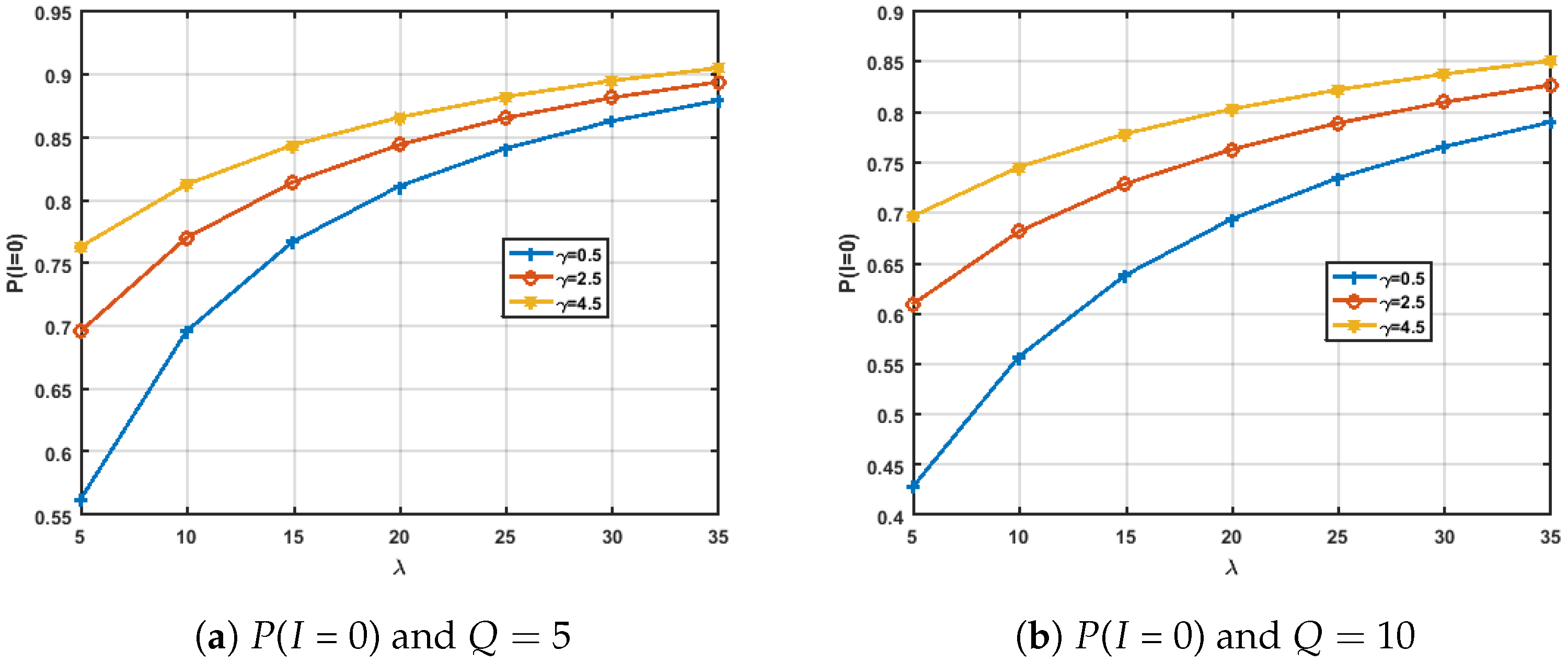
In terms of deterministic order size, the effect of adding the deterioration parameter $\gamma$ on $P\left(X\right(t)=0)$, referred to in Figure 3a,b, shows that for a constant Q value, the probability that the inventory being empty takes less value when the deterioration happens and vice versa makes sense as deterioration affects the availability of the items or the services for the customers. Furthermore, as can be seen, this measure increases as the customers arrive at the system and request a service or an item, as the number of items will decrease as it is given to the customer who requested the item or service. It was also noted that when the Q value increases, this measure decreases, which also makes sense as when the order quantity increases, the probability of the empty inventory decreases.

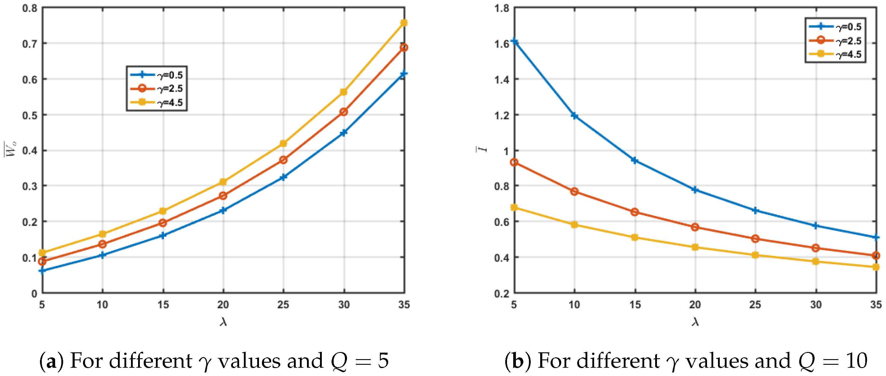
It was noticed that the dependency of $P\left(X\right(t)<Y(t\left)\right)$, $\overline{LS}$ and $\overline{L{S}_c}$ on the deterioration parameter $\gamma$ is increased as the value of Q increased. The relation between the parameters $\gamma$, Q, $\lambda$ and the mentioned measures have the same behavior as in the deterministic order size, as the only change was in the probability of delivering the items and services to the customers.

The visual representation of the effect of $\gamma$ on different measures with different $\lambda$ values under uniform order size is given in Figure 4a,b.

In this research, a limited number of $Y\left(t\right)-1$ waiting places of the integrated inventory-queuing model with deterioration was studied under uniformly distributed and deterministic order fixed quantity Q. In the proposed model, deterioration means falling from a higher to a lower level in quantity.

In the first instance, the Schwarz model was studied, modeled and analyzed under deterministic and uniformly distributed order quantity, depending on their mathematical approach in their article. The resulting performance measures found with the cost function have been presented. The same model that has been represented by the proposed method depends on finding a solution for the linear system found from generating the balance equations obtained from the drawn states of the desired system. After that, the generated model was analyzed and compared to the results obtained from examining the Schwarz model to ensure system validity. By analyzing the results, it was noticed that when the value of $\lambda$ increased, and for different values of Q, the performance measures such as $P\left(X\right(t)=0)$, $P\left(X\right(t)<Y(t\left)\right)$, $P\left(Y\right(t)=Y(t\left)\right)$, ${\lambda }_R$, ${\lambda }_A$, $\overline{LS}$, $\overline{L{S}_c}$, $\overline{L_0}$, $\overline{L}$, $\overline{W_o}$, $\overline{W}$ and F will be increased. There is no observed change in the values of the following measures, such as $P\left(Y\right(t)=0)$, $\overline{L{S}_c}$, $\overline{L_0}$ and $\overline{L}$. There is a critical value of $\lambda$ at which the cost function F changes its behavior, and it is approximately 23 in deterministic and 17 in uniformly distributed order size. At that point, the cost function values reversed from maximum to minimum and vice versa depending on the Q value.

A novel approach was used to analyze the performance measures of a limited integrated queuing-inventory model with deterioration parameter $\gamma$, which is exponentially distributed and has a value greater than Q under deterministic and uniform distributed order quantity. It was observed that the value of $\gamma$ increased, and for different values of $\lambda$, the performance measures such as $P\left(X\right(t)=0)$, ${\lambda }_R$, $\overline{W_o}$, and $\overline{W}$ expanded. Furthermore, it was noticed that the value of $\gamma$ increased, and for different values of $\lambda$, the performance measures such as $P\left(Y\right(t)=Y(t\left)\right)$, $\overline{X\left(t\right)}$, ${\lambda }_A$ and $\beta$ diminished. There was no observed change in $P\left(Y\right(t)=0)$, $P\left(X\right(t)<Y(t\left)\right)$, $\overline{LS}$, $\overline{L{S}_c}$, $\overline{L_0}$ and $\overline{L}$.

5. Conclusions

This research analyzes customers’ purification by examining the addition of deterioration parameter $\gamma$. The proposed model’s demand is based on Poisson, where service times and lead times are exponentially distributed. Schwarz $M/M/1/\infty$ and $M/M/1/N$-1-systems are further examined by employing the proposed method to solve the linear system of equations obtained from analyzing the steady-state system balance equations. The results obtained are compared with the empirical results by simulating the Schwarz approach. The analyzed model is tested for different values of Q, demand rate $\lambda$ and $\gamma$. The obtained results showed a substantial dependence between $\gamma$, Q and $\lambda$, delivering the required knowledge for decision-makers to achieve their objectives which depend on the performance measure of interest. In terms of uniform order size, the effect of increasing the deterioration parameter $\gamma$ on the performance measures under concentration, it was noticed that when the value of $\gamma$ increased, and for different values of $\lambda$, the performance measures such as $P\left(X\right(t)=0)$, ${\lambda }_R$, $\overline{W_o}$ and $\overline{W}$ tended to grow. Moreover, we also observed that the value of $\gamma$ increased, and for different values of $\lambda$, the performance measures such as $P\left(Y\right(t)=Y(t\left)\right)$, $\overline{X\left(t\right)}$, ${\lambda }_A$ and $\beta$ tended to drop. Furthermore, there is no observed change in $P\left(Y\right(t)=0)$, $P\left(X\right(t)<Y(t\left)\right)$, $\overline{LS}$, $\overline{L{S}_c}$, $\overline{L_0}$ and $\overline{L}$.

In future work, the system under consideration can be studied when changing $\mu$ or $\nu$ under different distributions. Furthermore, the effect of adding the deterioration parameter on the cost function can be further analyzed.

References

1. Khan, M.T.; Idrees, M.D.; Rauf, M.; Sami, A.; Ansari, A.; Jamil, A. Green Supply Chain Management Practices’ Impact on Operational Performance with the Mediation of Technological Innovation. Sustainability 2022, 14, 3362. [Google Scholar] [CrossRef]
2. Liu, P.; Hendalianpour, A.; Hamzehlou, M.; Feylizadeh, M. Cost Reduction of Inventory-Production-System in Multi-echelon Supply Chain Using Game Theory and Fuzzy Demand Forecasting. Int. J. Fuzzy Syst. 2022, 1–21. [Google Scholar] [CrossRef]
3. Quansah, F.; Ankomah, F.; Hagan, J.E., Jr.; Srem-Sai, M.; Frimpong, J.B.; Sambah, F.; Schack, T. Development and Validation of an Inventory for Stressful Situations in University Students Involving Coping Mechanisms: An Interesting Cultural Mix in Ghana. Psych 2022, 4, 15. [Google Scholar] [CrossRef]
4. Ijioui, R.; Emmerich, H.; Ceyp, M. Strategies and Tactics in Supply Chain Event Management; Springer: Berlin/Heidelberg, Germany, 2007. [Google Scholar]
5. Tiwari, S.; Cárdenas-Barrón, L.E.; Malik, A.I.; Jaggi, C.K. Retailer’s credit and inventory decisions for imperfect quality and deteriorating items under two-level trade credit. Comput. Oper. Res. 2022, 138, 105617. [Google Scholar] [CrossRef]
6. Schneeweiß, C. Einführung in die Produktionswirtschaft; Springer: Berlin/Heidelberg, Germany, 2013. [Google Scholar]
7. Stadtler, H.; Kilger, C. Supply Chain Management and Advanced Planning; Springer: Berlin/Heidelberg, Germany, 2002; Volume 4. [Google Scholar]
8. Melikov, A.; Shahmaliyev, M.; Nair, S. Matrix-Geometric Method for the Analysis of a Queuing System with Perishable Inventory. Autom. Remote Control. 2021, 82, 2169–2182. [Google Scholar] [CrossRef]
9. Jeganathan, K.; Harikrishnan, T.; Selvakumar, S.; Anbazhagan, N.; Amutha, S.; Acharya, S.; Dhakal, R.; Joshi, G.P. Analysis of Interconnected Arrivals on Queueing-Inventory System with Two Multi-Server Service Channels and One Retrial Facility. Electronics 2021, 10, 576. [Google Scholar] [CrossRef]
10. Karthikeyan, K.; Sudhesh, R. Recent review article on queueing inventory systems. Res. J. Pharm. Technol. 2016, 9, 2056. [Google Scholar] [CrossRef]
11. Alnowibet, K.A.; Alrasheedi, A.F.; Alqahtani, F.S. Queuing Models for Analyzing the Steady-State Distribution of Stochastic Inventory Systems with Random Lead Time and Impatient Customers. Processes 2022, 10, 624. [Google Scholar] [CrossRef]
12. Alnowibet, K.; Tadj, L. Analysis of Two Phases Queue With Vacations and Breakdowns Under T-Policy. In Advanced Methodologies and Technologies in Digital Marketing and Entrepreneurship; IGI Global: Hershey, PA, USA, 2019; pp. 13–31. [Google Scholar]
13. Wanger, H.; Lissan, A.; Holze, J.; Herhanmer, L. The incorporation of P32 into the inositol phosphatides of the rate brain. J. Lipid Res. 1962, 3, 177. [Google Scholar]
14. Hadley, G.; Whitin, T.M. Analysis of Inventory Systems; Technical Report; Prentice-Hall: Englewood Cliffs, NJ, USA, 1963. [Google Scholar]
15. Naddor, E. Inventory Systems; Technical Report; Wiley: New York, NY, USA, 1966. [Google Scholar]
16. Brown, R.G. Decision Rules for Inventory Management; FAO: Rome, Italy, 1967. [Google Scholar]
17. Eilon, S.; Lampkin, W. Inventory Control Abstracts (1953–1965); Oliver & Boyd: Edinburgh, Scotland, 1968. [Google Scholar]
18. Raafat, F. Survey of literature on continuously deteriorating inventory models. J. Oper. Res. Soc. 1991, 42, 27–37. [Google Scholar] [CrossRef]
19. MISRA, R.B. Optimum production lot size model for a system with deteriorating inventory. Int. J. Prod. Res. 1975, 13, 495–505. [Google Scholar] [CrossRef]
20. Bazan, E.; Jaber, M.Y.; Zanoni, S. A review of mathematical inventory models for reverse logistics and the future of its modeling: An environmental perspective. Appl. Math. Model. 2016, 40, 4151–4178. [Google Scholar] [CrossRef]
21. Sixta, J.; Žižka, M. Metody; Computer Press: Brno, Czech Republic, 2010. [Google Scholar]
22. Lee, Y.; Chan, C.K.; Langevin, A.; Lee, H. Integrated inventory-transportation model by synchronizing delivery and production cycles. Transp. Res. Part E Logist. Transp. Rev. 2016, 91, 68–89. [Google Scholar] [CrossRef]
23. Hollier, R.; Mak, K. Inventory replenishment policies for deteriorating items in a declining market. Int. J. Prod. Res. 1983, 21, 813–836. [Google Scholar] [CrossRef]
24. Mandal, B.A.; Phaujdar, S. An inventory model for deteriorating items and stock-dependent consumption rate. J. Oper. Res. Soc. 1989, 40, 483–488. [Google Scholar] [CrossRef]
25. Sandhu, B.S. A study on inventory of deteriorating things having price reliant demand, time reliant holding cost. J. Gujarat Res. Soc. 2019, 21, 522–528. [Google Scholar]
26. Indhumathy, N.; Jayashree, P. A Periodic Review Deterministic Inventory Model with Exponential Rate of Demand for Deteriorating Items and Partial Backlogging. Int. J. Comput. Theor. Stat. 2019, 6. [Google Scholar] [CrossRef]
27. Liu, M.; Feng, M.; Wong, C.Y. Flexible service policies for a Markov inventory system with two demand classes. Int. J. Prod. Econ. 2014, 151, 180–185. [Google Scholar] [CrossRef]
28. Schwarz, M.; Sauer, C.; Daduna, H.; Kulik, R.; Szekli, R. M/M/1 queueing systems with inventory. Queueing Syst. 2006, 54, 55–78. [Google Scholar] [CrossRef]
29. Krishnamoorthy, A.; Lakshmy, B.; Manikandan, R. A survey on inventory models with positive service time. Opsearch 2011, 48, 153–169. [Google Scholar] [CrossRef]
30. Sigman, K.; Simchi-Levi, D. Light traffic heuristic for anM/G/1 queue with limited inventory. Ann. Oper. Res. 1992, 40, 371–380. [Google Scholar] [CrossRef]
31. Berman, O.; Kim, E. Stochastic models for inventory management at service facilities. Stoch. Model. 1999, 15, 695–718. [Google Scholar] [CrossRef]
32. Berman, O.; Kim, E. Dynamic order replenishment policy in internet-based supply chains. Math. Methods Oper. Res. 2001, 53, 371–390. [Google Scholar] [CrossRef]
33. Berman, O.; Kim, E. Dynamic inventory strategies for profit maximization in a service facility with stochastic service, demand and lead time. Math. Methods Oper. Res. 2004, 60, 497–521. [Google Scholar] [CrossRef]
34. Berman, O.; Sapna, K. Optimal service rates of a service facility with perishable inventory items. Nav. Res. Logist. (NRL) 2002, 49, 464–482. [Google Scholar] [CrossRef]
35. Berman, O.; Sapna, K. Inventory management at service facilities for systems with arbitrarily distributed service times. Stoch. Model. 2000, 16, 343–360. [Google Scholar] [CrossRef]
36. Ding, S. Integration on corporate inventory under continuous demand. J. Interdiscip. Math. 2018, 21, 917–928. [Google Scholar] [CrossRef]
37. Mohebbi, E.; Posner, M.J. A continuous-review inventory system with lost sales and variable lead time. Nav. Res. Logist. (NRL) 1998, 45, 259–278. [Google Scholar] [CrossRef]
Figure 1. Integrated queuing-inventory model with lost sales.
Processes 10 00781 g001
Figure 2. M / M / 1 / N 1 -systems with inventory, lost sales and deterioration.
Processes 10 00781 g002
Figure 3. The effect of increasing demand ( λ ) for different γ values under deterministic order size.
Processes 10 00781 g003
Figure 4. The effect of increasing demand ( λ ) for different γ values under uniform order size.
Processes 10 00781 g004