
Artificial Neural Network for Fast and Versatile Model Parameter Adjustment Utilizing PAT Signals of Chromatography Processes for Process Control under Production Conditions

Abstract
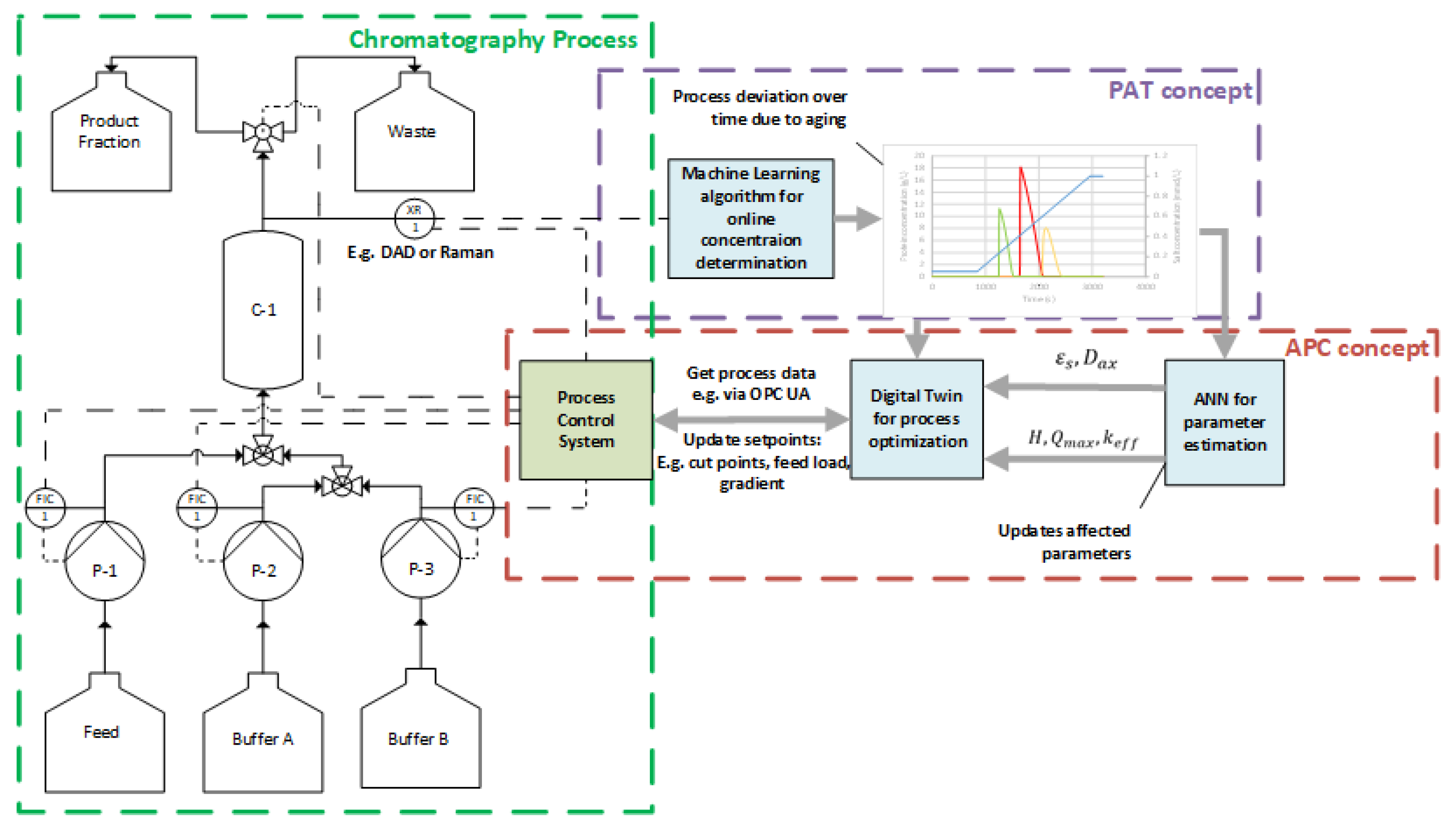
:1. Introduction
2. Materials and Methods
2.1. Chromatography Modeling
2.2. Model Parameter Choice and ANN Dataset Generation
3. Results
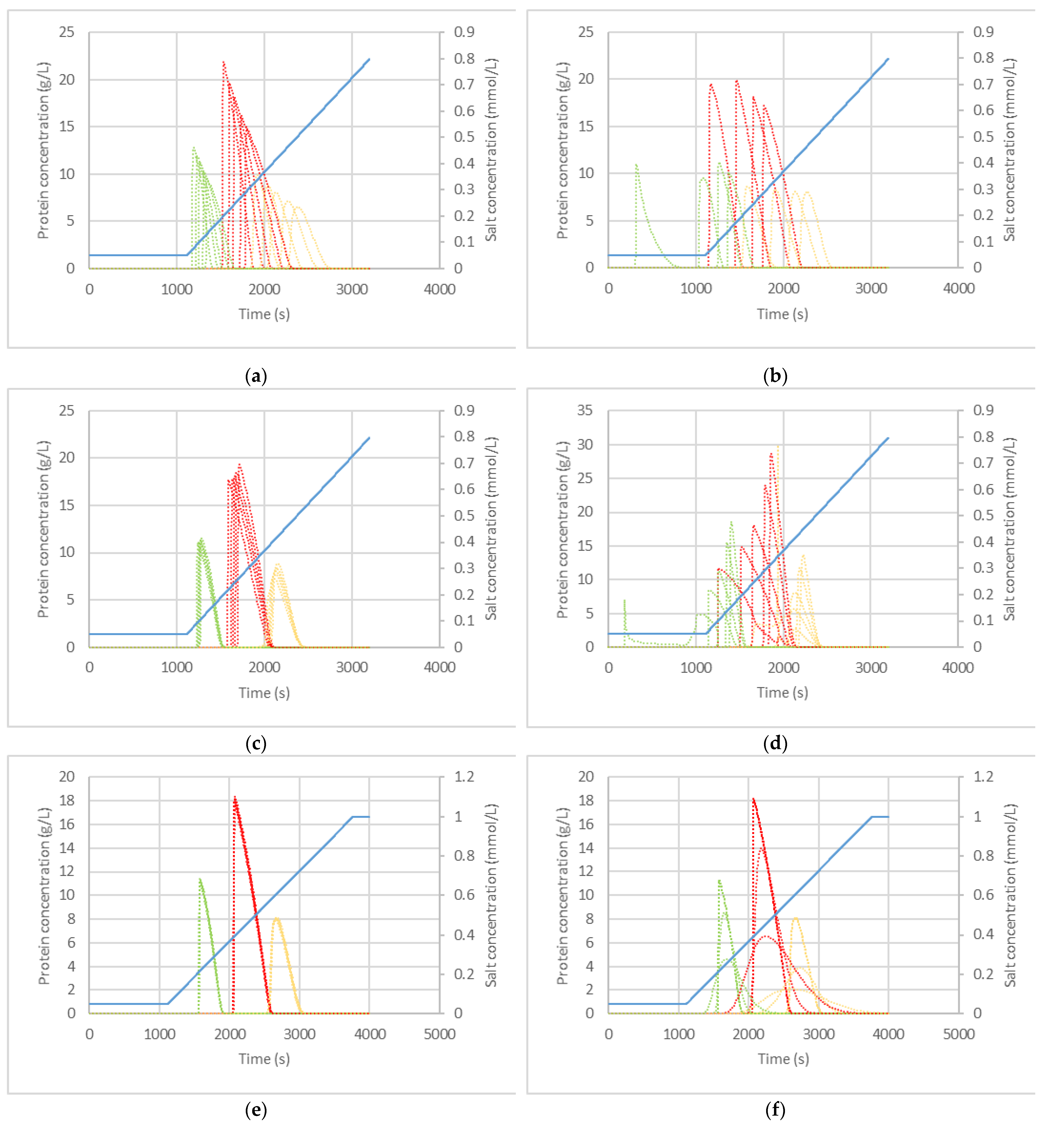
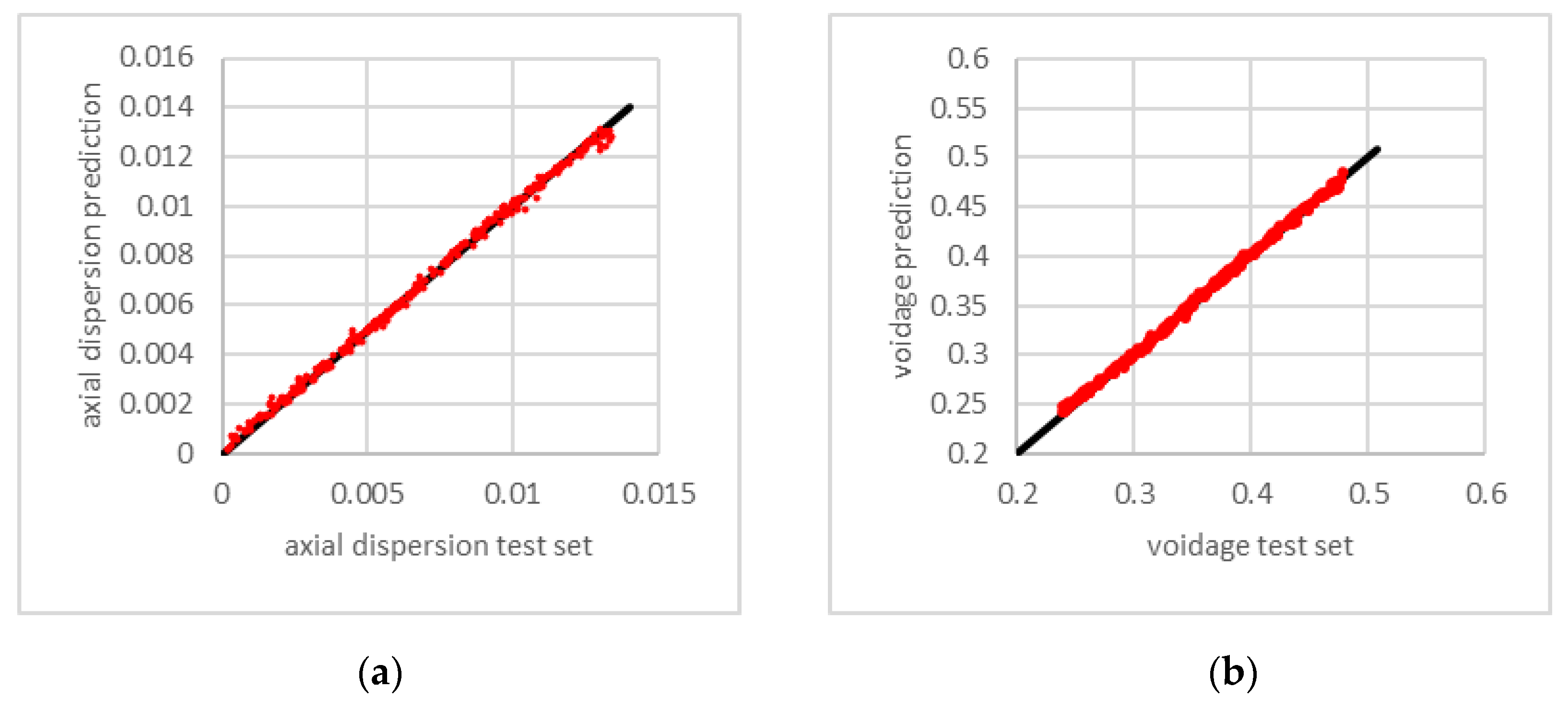
3.1. Variation of Packing and Fluid Dynamic Parameters
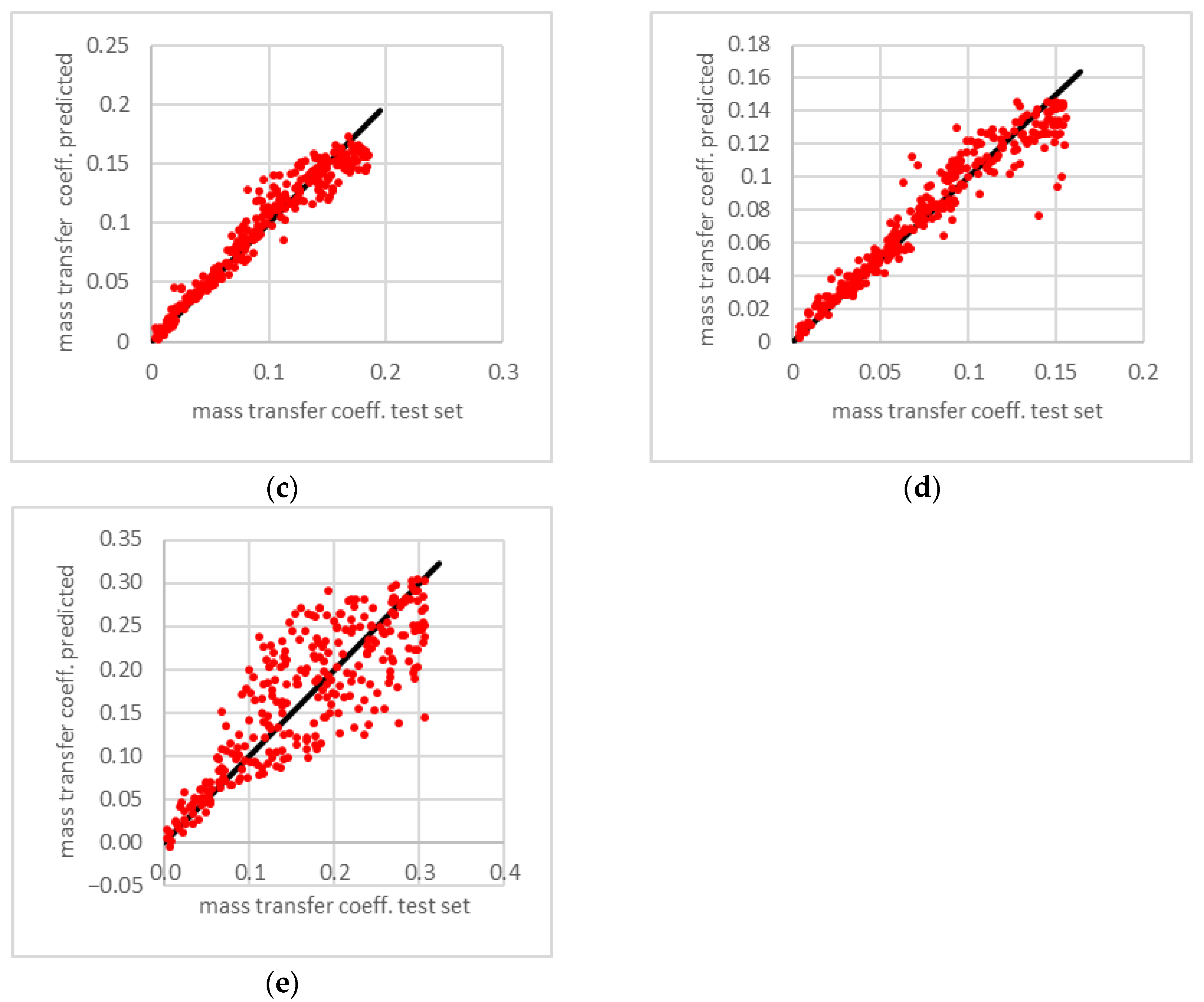
3.2. Variation of Phase Equilibrium Parameters
3.3. Variation of Phase Equilibrium, Fluid Dynamic and Packing Parameters at Once
4. Conclusions
Author Contributions
Funding
Institutional Review Board Statement
Informed Consent Statement
Data Availability Statement
Acknowledgments
Conflicts of Interest
References
- Hattori, Y.; Tajiri, Y.; Otsuka, M. Tablet Characteristics Prediction by Powder Blending Process Analysis Based on near Infrared Spectroscopy. J. Near Infrared Spectrosc. 2013, 21, 1–9. [Google Scholar] [CrossRef]
- Golubović, J.; Protić, A.; Zečević, M.; Otašević, B.; Mikić, M. Artificial neural networks modeling in ultra performance liquid chromatography method optimization of mycophenolate mofetil and its degradation products. J. Chemom. 2014, 28, 567–574. [Google Scholar] [CrossRef]
- Abadi, M.; Agarwal, A.; Barham, P.; Brevdo, E.; Chen, Z.; Citro, C.; Corrado, G.S.; Davis, A.; Dean, J.; Devin, M.; et al. Tensorflow: Large-Scale Machine Learning on Heterogeneous Distributed Systems. Available online: https://static.googleusercontent.com/media/research.google.com/en//pubs/archive/45166.pdf (accessed on 19 December 2021).
- The MathWorks Inc. MATLAB Statistics and Machine Learning Toolbox; The MathWorks Inc.: Natick, MA, USA, 2019. [Google Scholar]
- Fausett, L.V. Fundamentals of Neural Networks: Architectures, Algorithms, and Applications; Prentice Hall: Englewood Cliffs, NJ, USA, 1994; ISBN 0-13-334186-0. [Google Scholar]
- Gudivada, V.N.; Rao, C.R. (Eds.) Computational Analysis and Understanding of Natural Languages: Principles, Methods and Applications; Elsevier: Amsterdam, The Netherlands, 2018; ISBN 978-0-444-64042-0. [Google Scholar]
- Asprion, N.; Böttcher, R.; Pack, R.; Stavrou, M.-E.; Höller, J.; Schwientek, J.; Bortz, M. Gray-Box Modeling for the Optimization of Chemical Processes. Chem. Ing. Tech. 2019, 91, 305–313. [Google Scholar] [CrossRef]
- Hagge, T.; Stinis, P.; Yeung, E.; Tartakovsky, A.M. Solving differential equations with unknown constitutive relations as recurrent neural networks. arxiv 2017, arXiv:1710.02242. [Google Scholar]
- Gao, W.; Engell, S. Neural Network-Based Identification of Nonlinear Adsorption Isotherms. IFAC Proc. Vol. 2004, 37, 721–726. [Google Scholar] [CrossRef]
- Goodfellow, I.; Bengio, Y.; Courville, A. Deep Learning; MIT Press: Cambridge, MA, USA; London, UK, 2016; ISBN 978-0262035613. [Google Scholar]
- Wang, G.; Briskot, T.; Hahn, T.; Baumann, P.; Hubbuch, J. Estimation of adsorption isotherm and mass transfer parameters in protein chromatography using artificial neural networks. J. Chromatogr. A 2017, 1487, 211–217. [Google Scholar] [CrossRef]
- Mouellef, M.; Vetter, F.L.; Zobel-Roos, S.; Strube, J. Fast and Versatile Chromatography Process Design and Operation Optimization with the Aid of Artificial Intelligence. Processes 2021, 9, 2121. [Google Scholar] [CrossRef]
- Ley, C.; Elvers, B.; Bellussi, G.; Bus, J.; Drauz, K.; Greim, H.; Hessel, V.; Kleemann, A.; Kutscher, B.; Meijer, G.; et al. (Eds.) Ullmann’s Encyclopedia of Industrial Chemistry; Wiley: Chichester, UK, 2010; ISBN 3527306730. [Google Scholar]
- Golshan-Shirazi, S.; Guiochon, G. Optimization of experimental conditions in preparative liquid chromatography. J. Chromatogr. A 1991, 536, 57–73. [Google Scholar] [CrossRef]
- Ströhlein, G.; Aumann, L.; Müller-Späth, T.; Tarafder, A.; Morbidelli, M. CONTINUOUS PROCESSING: The Multiclomn Countercurrent Solvent Gradient Purification Process: A continuous chromatographic process for monoclonal antibodies without using Protein A. BioPharm Int. 2007, 22, 42–48. [Google Scholar]
- Godawat, R.; Brower, K.; Jain, S.; Konstantinov, K.; Riske, F.; Warikoo, V. Periodic counter-current chromatography—Design and operational considerations for integrated and continuous purification of proteins. Biotechnol. J. 2012, 7, 1496–1508. [Google Scholar] [CrossRef]
- Helling, C.; Dams, T.; Gerwat, B.; Belousov, A.; Strube, J. Physical characterization of column chromatography: Stringend control over equipment performance in biopharmaceutical production. Trends Chromatogr. 2013, 8, 55–71. [Google Scholar]
- International Council for Harmonisation of Technical Requirements for Pharmaceuticals for Human Use. ICH-Endorsed Guide for ICH Q8/Q9/Q10 Implementation. 6 December 2011. Available online: https://database.ich.org/sites/default/files/Q8_Q9_Q10_Q%26As_R4_Points_to_Consider_0.pdf (accessed on 28 February 2022).
- Zhang, J.; Siva, S.; Caple, R.; Ghose, S.; Gronke, R. Maximizing the functional lifetime of Protein A resins. Biotechnol. Prog. 2017, 33, 708–715. [Google Scholar] [CrossRef]
- Rathore, A.S.; Bracewell, D.G.; Phatak, M.; Ma, G. Re-use of Protein A Resin: Fouling and Economics. BioPharm Int. 2015, 28, 28–33. [Google Scholar]
- Andersson, J.A.E.; Gillis, J.; Horn, G.; Rawlings, J.B.; Diehl, M. CasADi: A software framework for nonlinear optimization and optimal control. Math. Prog. Comp. 2019, 11, 1–36. [Google Scholar] [CrossRef]
- Kornecki, M.; Schmidt, A.; Lohmann, L.; Huter, M.; Mestmäcker, F.; Klepzig, L.; Mouellef, M.; Zobel-Roos, S.; Strube, J. Accelerating Biomanufacturing by Modeling of Continuous Bioprocessing—Piloting Case Study of Monoclonal Antibody Manufacturing. Processes 2019, 7, 495. [Google Scholar] [CrossRef] [Green Version]
- Zobel-Roos, S.; Schmidt, A.; Mestmäcker, F.; Mouellef, M.; Huter, M.; Uhlenbrock, L.; Kornecki, M.; Lohmann, L.; Ditz, R.; Strube, J. Accelerating Biologics Manufacturing by Modeling or: Is Approval under the QbD and PAT Approaches Demanded by Authorities Acceptable Without a Digital-Twin? Processes 2019, 7, 94. [Google Scholar] [CrossRef] [Green Version]
- Bakeev, K.A. (Ed.) Process Analytical Technology: Spectroscopic Tools and Implementation Strategies for the Chemical and Pharmaceutical Industries; Blackwell: Oxford, UK, 2006; ISBN 1-4051-2103-3. [Google Scholar]
- Kessler, W. Multivariate Datenanalyse für die Pharma-, Bio- und Prozessanalytik: Ein Lehrbuch, 1st ed.; Wiley: Weinheim, Germany, 2008; ISBN 9783527312627. (In German) [Google Scholar]
- Rathore, A.S.; Kapoor, G. Application of process analytical technology for downstream purification of biotherapeutics. J. Chem. Technol. Biotechnol. 2015, 90, 228–236. [Google Scholar] [CrossRef]
- Großhans, S.; Rüdt, M.; Sanden, A.; Brestrich, N.; Morgenstern, J.; Heissler, S.; Hubbuch, J. In-line Fourier-transform infrared spectroscopy as a versatile process analytical technology for preparative protein chromatography. J. Chromatogr. A 2018, 1547, 37–44. [Google Scholar] [CrossRef]
- van Rossum, G. The Python Language Reference, Release 3.0.1 [Repr.]; Python Software Foundation: Hampton, NH, USA; SoHo Books: Redwood City, CA, USA, 2010; ISBN 1441412697. [Google Scholar]
- Spyder IDE. Available online: https://www.spyder-ide.org/ (accessed on 19 December 2021).
- Keras. Available online: https://keras.io (accessed on 19 December 2021).
- Guiochon, G. Fundamentals of Preparative and Nonlinear Chromatography, 2nd ed.; Elsevier: Amsterdam, The Netherlands, 2006; ISBN 978-0123705372. [Google Scholar]
- Shekhawat, L.K.; Rathore, A.S. An overview of mechanistic modeling of liquid chromatography. Prep. Biochem. Biotechnol. 2019, 49, 623–638. [Google Scholar] [CrossRef]
- Carta, G.; Rodrigues, A.E. Diffusion and convection in chromatographic processes using permeable supports with a bidisperse pore structure. Chem. Eng. Sci. 1993, 48, 3927–3935. [Google Scholar] [CrossRef]
- Wilson, E.J.; Geankoplis, C.J. Liquid Mass Transfer at Very Low Reynolds Numbers in Packed Beds. Ind. Eng. Chem. Fund. 1966, 5, 9–14. [Google Scholar] [CrossRef]
- Carta, G.; Jungbauer, A. Protein Chromatography; Wiley: Weinheim, Germany, 2010; ISBN 9783527318193. [Google Scholar]
- Seidel-Morgenstern, A.; Guiochon, G. Modelling of the competitive isotherms and the chromatographic separation of two enantiomers. Chem. Eng. Sci. 1993, 48, 2787–2797. [Google Scholar] [CrossRef]
- Leśko, M.; Åsberg, D.; Enmark, M.; Samuelsson, J.; Fornstedt, T.; Kaczmarski, K. Choice of Model for Estimation of Adsorption Isotherm Parameters in Gradient Elution Preparative Liquid Chromatography. Chromatographia 2015, 78, 1293–1297. [Google Scholar] [CrossRef] [PubMed] [Green Version]
- Mollerup, J.M. A Review of the Thermodynamics of Protein Association to Ligands, Protein Adsorption, and Adsorption Isotherms. Chem. Eng. Technol. 2008, 31, 864–874. [Google Scholar] [CrossRef]
- Brooks, C.A.; Cramer, S.M. Steric mass-action ion exchange: Displacement profiles and induced salt gradients. AIChE J. 1992, 38, 1969–1978. [Google Scholar] [CrossRef]
- Langmuir, I. The adsorption of gases on plane surfaces of glass, mica and platinum. J. Am. Chem. Soc. 1918, 40, 1361–1403. [Google Scholar] [CrossRef] [Green Version]
- Zobel-Roos, S. Entwicklung, Modellierung und Validierung von integrierten kontinuierlichen Gegenstrom-Chromatographie-Prozessen. Ph.D. Thesis, Shaker Verlag GmbH, Clausthal University of Technologies, Clausthal-Zellerfeld, Germany, 2018. [Google Scholar]
- Seidel-Morgenstern, A. Experimental determination of single solute and competitive adsorption isotherms. J. Chromatogr. A 2004, 1037, 255–272. [Google Scholar] [CrossRef]
- Zobel-Roos, S.; Mouellef, M.; Ditz, R.; Strube, J. Distinct and Quantitative Validation Method for Predictive Process Modelling in Preparative Chromatography of Synthetic and Bio-Based Feed Mixtures Following a Quality-by-Design (QbD) Approach. Processes 2019, 7, 580. [Google Scholar] [CrossRef] [Green Version]
- Young, M.E.; Carroad, P.A.; Bell, R.L. Estimation of diffusion coefficients of proteins. Biotechnol. Bioeng. 1980, 22, 947–955. [Google Scholar] [CrossRef]
- Chung, S.F.; Wen, C.Y. Longitudinal dispersion of liquid flowing through fixed and fluidized beds. AIChE J. 1968, 14, 857–866. [Google Scholar] [CrossRef]


| Parameter | Lower Bound | Initial | Upper Bound |
|---|---|---|---|
Publisher’s Note: MDPI stays neutral with regard to jurisdictional claims in published maps and institutional affiliations. |
© 2022 by the authors. Licensee MDPI, Basel, Switzerland. This article is an open access article distributed under the terms and conditions of the Creative Commons Attribution (CC BY) license (https://creativecommons.org/licenses/by/4.0/).
Share and Cite
Mouellef, M.; Szabo, G.; Vetter, F.L.; Siemers, C.; Strube, J. Artificial Neural Network for Fast and Versatile Model Parameter Adjustment Utilizing PAT Signals of Chromatography Processes for Process Control under Production Conditions. Processes 2022, 10, 709. https://doi.org/10.3390/pr10040709
Mouellef M, Szabo G, Vetter FL, Siemers C, Strube J. Artificial Neural Network for Fast and Versatile Model Parameter Adjustment Utilizing PAT Signals of Chromatography Processes for Process Control under Production Conditions. Processes. 2022; 10(4):709. https://doi.org/10.3390/pr10040709
Chicago/Turabian StyleMouellef, Mourad, Glaenn Szabo, Florian Lukas Vetter, Christian Siemers, and Jochen Strube. 2022. "Artificial Neural Network for Fast and Versatile Model Parameter Adjustment Utilizing PAT Signals of Chromatography Processes for Process Control under Production Conditions" Processes 10, no. 4: 709. https://doi.org/10.3390/pr10040709