Modeling and Optimal Control of an Electro-Fermentation Process within a Batch Culture

Abstract

Electro-fermentation is a novel process that consists in coupling a microbial fermentative metabolism with an electrochemical system. In such a process, the electrodes act either as the electron sinks or sources modifying the fermentation balance of a microbial fermentative metabolism and provide new options for the control of microbial activity. A theoretical framework for the analysis and control of fermentations using electro-fermentation is currently lacking. In this paper, we propose a simple electro-fermentation model in which a population of fermentative bacteria switch between two metabolic behaviors in response to different electrode potentials. We then mathematically analyze optimal strategies to maximize the production of one of the rising products in a batch fermentation using Pontryagin’s Maximum Principle. The obtained results show that, in some experimental configurations, a dynamic control of the electrode potential is required for the maximization of the desired product. Consequences of the obtained optimal strategy for driving electro-fermentation experiments are discussed through a realistic example. This analysis also highlights that the transition rates between fermentation and electro-fermentation behaviors are currently unknown and would be crucial to quantify in order to apply such a control approach.

1. Introduction

The knowledge of electroactive microorganisms has rapidly grown over the last 20 years with the development of microbial electrochemical technologies such as microbial fuel cells (MFC) and microbial electrolysis cells (MEC) for the production of electricity or hydrogen from organic matter [1]. The development of electromicrobiology has also led to several promising applications, such as electro-fermentation (EF) in which reducing power provided by means of an electrode can redirect fermentation pathways [2]. In that case, the electrodes act as either the electron sinks or sources modifying the fermentation balance of a microbial fermentative metabolism, providing new options for the control of microbial communities [3,4]. EF has been successfully applied on mixed culture fermentations and pure culture fermentations and has proven efficient for increasing yields in various products such as hydrogen, acetate, propionate, butyrate, lactate, 3-hydroxypropanoic acid, ethanol, 1.3-propanediol, 2,3-butandiol, butanol, or acetone [5,6,7,8,9,10,11,12,13,14,15,16]. For example, a metabolic shift occurred in Clostridium pasteurianum when taking up electrons from an electrode poised at +0.045 V vs. SHE (standard hydrogen electrode) with an increased production of reduced products such as butanol from glucose and 1.3-propanediol from glycerol [12]. From a biotechnological point of view, EF could lead to significant improvements of industrial fermentations using only a small amount of electrical power. Moreover, the use of an electrode for the triggering of the EF effect in the fermentation system introduce the possibility of a dynamic control of fermentation. However, mathematical models describing the EF effect are currently lacking. In EF, the voltage applied between electrodes is a variable that could be adjusted dynamically, typically with the objective of maximizing the total production over a time interval. We shall state and study such an optimization problem with the help of the theory of optimal control, for which several analytical and numerical tools are available. Optimal control has been successfully applied to various bioprocesses, providing practical control strategies, mostly in terms of feedback control (e.g., [17]), as we shall consider here.

Here we consider a pure culture of a fermentative microorganism growing on a limiting resource in a batch culture. As described above, the application of an external potential through the implementation of an electrode in the bioreactor leads to a switching of the metabolism between two different metabolic pathways. This EF effect is modeled by considering two microbial subpopulations producing different metabolites $(f_1,f_2)$ giving rise to two different products ($s_1,s_2$). The switching between the fermentation behaviors depends on the electrode potential V (see Figure 1). The control parameter is simply chosen in such a way that its variation between two constants values (which correspond to two different values of V) leads to a transition between the two considered metabolic behaviors. The bioreactor equations in batch culture are simply used to establish the model [18]. Based on this model, an optimal control problem for the maximization of the production of $s_2$ is formulated. The Pontryagin’s Maximum Principle [17,19] is applied for the design of the optimal control strategy. The obtained results show that the optimal strategy is not trivial, in the sense that the control is not always constant (equal to that which correspond to $f_2$), where in some cases the metabolic behavior $f_1$ should be visited by the fermentative bacteria. The present mathematical analysis of the optimal strategies will serve as an experimental guide to design relevant experiments for testing if these strategies are eventually better, and thus contribute to the validation of the model.

The paper is organized as follows. In Section 2, we give the electro-fermentation model and introduce the optimization problem. A preliminary result analyzing the behavior of the optimal control in the case of proportional growth functions is given in Section 3. The main part of the paper is devoted to the synthesis of an optimal control strategy in two cases: case of identical growth functions in Section 4 and case of constant growth functions in Section 5. Finally, discussion and numerical simulations are given in Section 6.

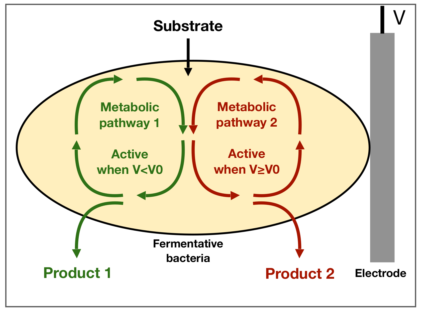
2. Model Description and Optimization Problem

In order to describe the switching between the two metabolic pathways described in the introduction, we suppose that the fermentative population is split into two sub-populations, $x_1$ and $x_2$, in a commensal relationship to consume substrate s. The sub-population $x_1$ with microbial growth rate ${\mu }_1$ gives rise to a product $s_1$ and the sub-population $x_2$ with microbial growth rate ${\mu }_2$ gives rise to a product $s_2$. We suppose that in the absence of polarized electrodes, the fermentation is mainly guided by the population $x_1$ and when the external voltage is sufficiently large, the metabolic function switches to a metabolism guided by $x_2$. This electro-fermentation process can be described by the following system of ordinary differential equations:

$$\begin{array}{ccc}\dot{s}\hfill & =\hfill & -\frac{1}{Y_1}{\mu }_1\left(s\right)x_1-\frac{1}{Y_2}{\mu }_2\left(s\right)x_2\hfill \\ {\dot{x}}_1\hfill & =\hfill & {\mu }_1\left(s\right)x_1-\alpha r_1{x}_1+(1-\alpha )r_2{x}_2\hfill \\ {\dot{x}}_2\hfill & =\hfill & {\mu }_2\left(s\right)x_2+\alpha r_1{x}_1-(1-\alpha )r_2{x}_2\hfill \end{array}$$

(1)

where $Y_1,Y_2$ are the yields coefficients, $r_1$, $r_2>0$ are positive constants, and $\alpha \in \{0,1\}$ is a control variable that is directly related to the external potential V and satisfies the following property:

$$\begin{array}{c}\hfill \alpha =0 \mathrm{i}\mathrm{f} V<V_0,\mathrm{and}\alpha =1 \mathrm{i}\mathrm{f} V\ge V_0,\end{array}$$

(2)

where $V_0>0$ is a threshold on the external potential over which the metabolic pathway is guided by $x_2$. The value of the threshold potential $V_0$ depends on the microorganisms $x_1$ and $x_2$. We shall assume that growths do not present inhibition, which amounts one to consider the following hypothesis.

Assumption 1.

The growth functions ${\mu }_i$ are non decreasing with ${\mu }_i\left(s\right)>0$ for $s>0$.

A classical model for the growth rates kinetics ${\mu }_i$ is given by the following Monod type functions:

$${\mu }_i\left(s\right)=\frac{k_{i}s}{K_i+s},i=1,2$$

(3)

for some positive real numbers $k_i,K_i$, for $i=1,2$.

Observe that, due to the migration phenomenon between the two sub-populations, the relation between $x_1$ and $x_2$ is not simply reduced to a competition phenomenon.

We shall assume that the two sub-populations have the same conversion factor.

Assumption 2.

$Y_1=Y_2=Y$.

Note that at the price of change of units of $x_1$ and $x_2$, one can without loss of generality assume that $Y=1$; this is conventional when dealing with chemostat type systems [20]. Therefore, we shall consider the simpler model:

$$\begin{array}{ccc}\dot{s}\hfill & =\hfill & -{\mu }_1\left(s\right)x_1-{\mu }_2\left(s\right)x_2\hfill \\ {\dot{x}}_1\hfill & =\hfill & {\mu }_1\left(s\right)x_1-\alpha r_1{x}_1+(1-\alpha )r_2{x}_2\hfill \\ {\dot{x}}_2\hfill & =\hfill & {\mu }_2\left(s\right)x_2+\alpha r_1{x}_1-(1-\alpha )r_2{x}_2,\hfill \end{array}$$

(4)

where $(s\left(0\right),x_1\left(0\right),x_2\left(0\right))=(s_0,x_{10},x_{20})\in {({\mathbb{R}}_{+}\setminus \left\{0\right\})}^3$. Observe that one has $s\left(t\right)+x_1\left(t\right)+x_2\left(t\right)=s\left(0\right)+x_1\left(0\right)+x_2\left(0\right):=c>0$ at any $t\ge 0$. Therefore, we can consider the reduced dynamics in the plane:

$$\begin{array}{ccc}{\dot{x}}_1\hfill & =\hfill & {\mu }_1(c-x_1-x_2)x_1-\alpha r_1{x}_1+(1-\alpha )r_2{x}_2\hfill \\ {\dot{x}}_2\hfill & =\hfill & {\mu }_2(c-x_1-x_2)x_2+\alpha r_1{x}_1-(1-\alpha )r_2{x}_2.\hfill \end{array}$$

(5)

The objective is to maximize the total production of the sub-population $x_2$ over an interval of time $[0,T]$, among functions $\alpha \left(·\right)$ that are measurable time functions taking values in $\{0,1\}$, which amounts to maximize the criterion:

$$J\left[\alpha \left(·\right)\right]={\int }_0^T{\mu }_2\left(s\left(t\right)\right)x_2\left(t\right)dt,$$

(6)

where $T>0$ is a fixed finite time horizon.

Remark 1.

From the condition given by (2), the control variable α is constrained to take values in the non-convex set $\{0,1\}$. In this case, one can not a priori guarantee the existence of optimal solutions for the problem (5) and (6). However, a technical approach consists of first considering the convexified problem, i.e., solve the problem with α taking values in the whole interval $[0,1]$, for which the existence of solutions is guaranteed (see for instance [21]). Then, the optimal solution can be approached with an arbitrary precision via chattering controls [22], which consist in commuting rapidly between the values 0 and 1 so that the averaged dynamics behave close from that one with α different from 0 and 1.

We shall use the Maximum Principle of Pontryagin (PMP) [19] to obtain necessary optimality conditions. Defining the Hamiltonian:

$$\begin{array}{c}\hfill H(x,p,\alpha )=p_1{\mu }_1(c-x_1-x_2)x_1+(p_2+1){\mu }_2(c-x_1-x_2)x_2\\ \hfill +(p_2-p_1)(\alpha r_1{x}_1-(1-\alpha )r_2{x}_2),\end{array}$$

(7)

where $p=(p_1,p_2)$ is the adjoint vector, the Pontryagin Maximum Principle claims that for any optimal solution, there exists an absolutely continuous function $p:[0,T]\to {\mathbb{R}}^2$ solution of the adjoint equation:

$$\dot{p}\left(t\right)=-{\partial }_{x}H(x\left(t\right),p\left(t\right),\alpha \left(t\right)),\mathrm{a}.\mathrm{e}.t\in [0,T]$$

(8)

with the terminal condition:

$$p\left(T\right)=0$$

(9)

and an optimal control ${\alpha }^{☆}$ that satisfy the maximization of the Hamiltonian:

$$\overline{H}(x\left(t\right),p\left(t\right)):=\underset{\alpha }{max}H(x\left(t\right),p\left(t\right),\alpha )=H(x\left(t\right),p\left(t\right),{\alpha }^{*}\left(t\right)),\mathrm{a}.\mathrm{e}.t\in [0,T].$$

(10)

In addition, the map $t\mapsto \overline{H}(x^{*}\left(t\right),p^{*}\left(t\right))$ is constant. Let:

$$\varphi \left(t\right)=p_2\left(t\right)-p_1\left(t\right)$$

(11)

be the switching function. From the maximization of the Hamiltonian, one gets the property for an optimal control:

$${\alpha }^{*}\left(t\right)=\left\{\begin{array}{c}1\mathrm{if}\varphi \left(t\right)>0,\hfill \\ 0\mathrm{if}\varphi \left(t\right)<0,\hfill \end{array}\right.\mathrm{a}.\mathrm{e}.t\ge 0 \mathrm{such\; that}\varphi \left(t\right)\ne 0.$$

(12)

3. Sufficient Condition for the Absence of Singular Arc

In this section, we give a sufficient condition under which any optimal solution of problem (5) and (6) does not admit a singular arc. Recall that a singular arc is a piece of an optimal trajectory for which the switching function $\varphi$ given by (11) vanishes in an interval of time $[t_1,t_2]$, for some $t_2>t_1\ge 0$. In that case, the maximization of the Hamiltonian (7) over $[t_1,t_2]$ becomes more difficult to study and additional techniques need to be involved in order to solve the problem on $[t_1,t_2]$. Accordingly to Remark 1, we can guarantee in absence of the singular arc that the optimal solution is reached with $\alpha$ taking only values 0 and 1 (even though the number of switches might be large or infinite).

Suppose that the growth rate functions satisfy the following assumption.

Assumption 3.

There exists a positive real $a\ne 1$ such that ${\mu }_1\left(s\right)=a{\mu }_2\left(s\right)$, for $s\ge 0$.

Note that Assumption 3 is not unrealistic. Indeed, when the growth rates follow the Monod expression (3), the linear approximation:

$${\mu }_i\left(s\right)\simeq \frac{k_i}{K_i}s(i=1,2)$$

is valid for relatively small values of s.

One has the following proposition.

Proposition 1.

Suppose that Assumption 3 holds. An optimal solution of the problem (4)–(6) has no singular arc.

Proof. 

The adjoint equations are:

$$\begin{array}{ccc}{\dot{p}}_1\hfill & =\hfill & -p_1{\mu }_1\left(s\right)+p_1{\mu }_1^{\prime }\left(s\right)x_1+(p_2+1){\mu }_2^{\prime }\left(s\right)x_2-\alpha r_1(p_2-p_1)\hfill \\ {\dot{p}}_2\hfill & =\hfill & -(p_2+1){\mu }_2\left(s\right)+p_1{\mu }_1^{\prime }\left(s\right)x_1+(p_2+1){\mu }_2^{\prime }\left(s\right)x_2+(1-\alpha )r_2(p_2-p_1)\hfill \end{array}$$

(13)

with $s=c-x_1-x_2$. If $\varphi =0$ on a time interval, one has $p_1=p_2$ and $\dot{\varphi }=0$, which gives:

$$p_1=a(p_2+1).$$

Therefore, $p_1$, $p_2$ have to be constant on this time interval, given by:

$$p_1=p_2=\frac{a}{1-a}.$$

Then, ${\dot{p}}_1={\dot{p}}_2=0$ gives the equations:

$$\begin{array}{c}{p}_1{\mu }_1^{\prime }\left(s\right)x_1+(p_2+1){\mu }_2^{\prime }\left(s\right)x_2=p_1{\mu }_1\left(s\right)\hfill \\ p_1{\mu }_1^{\prime }\left(s\right)x_1+(p_2+1){\mu }_2^{\prime }\left(s\right)x_2=(p_2+1){\mu }_2\left(s\right)\hfill \end{array}$$

from which we obtain that $p_1{\mu }_1\left(s\right)=(p_2+1){\mu }_2\left(s\right)$. Replacing $p_1$, $p_2$ by their expression and using Assumption 3, we obtain that $a=1$ and is thus a contradiction. □

Thanks to Proposition 1, the optimal control of problem (5) and (6) is a sequence of commutation between $\alpha =0$ and $\alpha =1$.

4. Optimal Synthesis with Identical Growth Functions

We investigate here the simple case for which one can assume that the two sub-populations have exactly the same growth rate. Such an assumption might be considered quite unrealistic. However, it could occur that growth rates are quite close to each other when the concentration s is not too large, which could then justify this assumption as a good approximation.

Proposition 2.

Consider the problem (5) and (6) and let $T>0$. Assume that one has ${\mu }_1\left(s\right)={\mu }_2\left(s\right):=\mu \left(s\right)$ for any $s>0$. Then, the constant control ${\alpha }^{☆}\equiv 1$ is optimal on $[0,T]$.

Proof. 

Let $b=x_1+x_2$. Then $b\left(·\right)$ is the solution of:

$$\dot{b}=\mu (c-b)b,b\left(0\right)=x_1\left(0\right)+x_2\left(0\right)$$

(14)

whatever is the control $\alpha \left(·\right)$. Then, the variable $X_2=x_2/b$ is the solution of:

$${\dot{X}}_2=\alpha r_1(1-X_2)-(1-\alpha )r_2{X}_2,X_2\left(0\right)=x_2\left(0\right)/(x_1\left(0\right)+x_2\left(0\right)).$$

(15)

Note that at any time t, ${\dot{X}}_2$ is maximal for $\alpha =1$, whatever is $X_2\in [0,1]$. Let ${\overline{X}}_2\left(·\right)$ be the solution for the control $\alpha$ identically equal to 1. From standard results of comparing solutions of scalar ordinary equations, one has $X_2\left(t\right)\le {\overline{X}}_2\left(t\right)$ at any t, whatever is the control $\alpha \left(·\right)$. Therefore, one has:

$$J\left[\alpha \left(·\right)\right]={\int }_0^T\mu (c-b\left(t\right))b\left(t\right)X_2\left(t\right)dt\le {\int }_0^T\mu (c-b\left(t\right))b\left(t\right){\overline{X}}_2\left(t\right)dt=J\left[1\right]$$

and we conclude that the constant control ${\alpha }^{☆}=1$ is optimal. □

Proposition 2 shows that, in the case of identical growth functions, the optimal strategy in order to maximize (6) is by keeping $\alpha$ constantly equal to one, i.e., by keeping an external potential sufficiently larger than $V_0$.

5. Optimal Synthesis with Constant Growth Functions

We consider here distinct growth rates, however we assume it to be constant for non-null concentration s.

Assumption 4.

One has ${\mu }_i\left(s\right)=a_i>0$ for any $s>0$ ($i=1,2$).

Indeed, if one considers that population growths follows the classical Monod function (3) and that the concentration $s\left(0\right)$ is quite large, having ${\mu }_i\left(s\right)=a_i$ can be a good approximation on the finite time horizon $[0,T]$ (provided T not to be too large).

The following the definition will be useful in the following.

Definition 1.

Denote $L=\frac{a_1}{a_2}$ and $K=\frac{r_1-a_1}{a_2}$ and define:

$$\tilde{\varphi }\left(p_2\right)=\left\{\begin{array}{cc}{\displaystyle \frac{K+L-K(L-1)p_2-(L+K){(p_2+1)}^{-K}}{K(K+1)}}\hfill & K\notin \{-1,0\}\hfill \\ (1-L)p_2+Llog(p_2+1)\hfill & K=0\hfill \\ -L+L(p_2+1)+log(p_2+1)(1-L)\hfill & K=-1\hfill \end{array}\right.$$

(16)

Define also, when $L>1$, the number:

$$\overline{\tau }:=\frac{log\left(inf\left\{p_2>0;\tilde{\varphi }\left(p_2\right)<0\right\}+1\right)}{a_2}.$$

(17)

Remark 2.

One can straightforwardly check that when $L>1$ (that is when $a_1>a_2$) one has:

$$\underset{p_2\to +\infty }{lim}\tilde{\varphi }\left(p_2\right)=-\infty$$

whatever is $K>-L$ (i.e., $r_1>0$). We deduce that $\overline{\tau }$ is well defined.

On has the following result.

Proposition 3.

Suppose that Assumption 4 holds. Consider the problem (5) and (6) and let $T>0$. One has the following two cases:

• If $a_1\le a_2$, then ${\alpha }^{☆}=1$ is optimal on $[0,T]$.
• If $a_1>a_2$, then the control:

  $${\alpha }^{☆}\left(t\right)=\left\{\begin{array}{cc}1\hfill & ift\ge min(0,T-\overline{\tau })\hfill \\ 0\hfill & otherwise\hfill \end{array}\right.$$

  is optimal on $[0,T]$.

Proof. 

The adjoint equations are written:

$$\begin{array}{ccc}{\dot{p}}_1\hfill & =\hfill & -a_1{p}_1-\alpha r_1(p_2-p_1)\hfill \\ {\dot{p}}_2\hfill & =\hfill & -a_2(p_2+1)+(1-\alpha )r_2(p_2-p_1).\hfill \end{array}$$

(18)

Note that system (18) is decoupled from the dynamics of $x_1$, $x_2$ and can be studied independently to the initial condition $(x_1\left(0\right),x_2\left(0\right))$. The switching function satisfies:

$$\dot{\varphi }=-a_2+a_1{p}_1-a_2{p}_2+\varphi \left(r_2+\alpha (r_1-r_2)\right).$$

(19)

At terminal time T, one has $\varphi \left(T\right)=0$ with $\dot{\varphi }\left(T\right)=-a_2<0$. So we conclude about the existence of the number:

$${\overline{t}}_1:=inf\left\{t>0;\varphi \left(\tau \right)>0,\tau \in (t,T)\right\}$$

and the optimality of $\alpha =1$ on the interval $[{\overline{t}}_1,T]$. On this interval, one has:

$$\begin{array}{ccc}{\dot{p}}_2\hfill & =\hfill & -a_2(p_2+1)\hfill \\ \dot{\varphi }\hfill & =\hfill & -a_2+(a_1-a_2)p_2+(r_1-a_1)\varphi .\hfill \end{array}$$

(20)

Note that $p_2\left(T\right)=0$ implies that one has necessarily $p_2>0$ on $[{\overline{t}}_1,T)$.

If $a_1\le a_2$, $\varphi$ cannot cross 0 from below because $\varphi =0$ implies $\dot{\varphi }<0$. We deduce from (20) that $\varphi$ is negative on $[{\overline{t}}_1,T)$, and thus ${\overline{t}}_1$ has to be equal to 0. We conclude that ${\alpha }^{☆}=1$ is optimal on $[0,T]$.

Consider now the case $a_1>a_2$. Let us show that an optimal solution cannot present a singular arc, i.e., a time interval on which $\varphi$ is identically null. If not, $\dot{\varphi }=0$ and $\varphi =0$ implies from Equation (19) that $p_2$ has to be constant on such an interval with $p_2=a_2/(a_1-a_2)>0$. However, from Equation (18) with ${\dot{p}}_2=0$ and $p_2=p_1$, one obtains $p_2=-1<0$, and thus a contradiction. We deduce that an optimal solution is a concatenation of arcs with $\alpha =0$ or $\alpha =1$. Note, from Equation (19), that $\dot{\varphi }$ is continuous at switching times (with $\dot{\varphi }=-a_2+(a_1-a_2)p_2=-a_2+(a_1-a_2)p_1$). If ${\overline{t}}_1>0$, we consider the number:

$${\overline{t}}_0:=inf\left\{t>0;\varphi \left(\tau \right)<0,\tau \in (t,{\overline{t}}_1)\right\}.$$

On the interval $({\overline{t}}_0,{\overline{t}}_1)$, $\alpha =0$ is optimal and one has:

$$\begin{array}{ccc}{\dot{p}}_1\hfill & =\hfill & -a_1{p}_1\hfill \\ \dot{\varphi }\hfill & =\hfill & -a_2+(a_1-a_2)p_1+(r_2-a_2)\varphi .\hfill \end{array}$$

(21)

Note that one has $p_1\left({\overline{t}}_1\right)=p_2\left({\overline{t}}_1\right)>0$, which implies $p_1\left(t\right)>p_1\left({\overline{t}}_1\right)$ for $t\in [{\overline{t}}_0,{\overline{t}}_1)$. As $\varphi$ changes its sign at ${\overline{t}}_1$ (from negative to positive values), one has necessarily $\dot{\varphi }\left({\overline{t}}_1\right)\ge 0$ (with $\varphi \left({\overline{t}}_1\right)=0$). If ${\overline{t}}_0>0$, one should have $\varphi \left({\overline{t}}_0\right)=0$ with $\dot{\varphi }\left({\overline{t}}_0\right)=-a_2+(a_1-a_2)p_1\left({\overline{t}}_0\right)>-a_2+(a_1-a_2)p_1\left({\overline{t}}_1\right)=\dot{\varphi }\left({\overline{t}}_1\right)\ge 0$, which contradicts the change of sign of $\varphi$ at ${\overline{t}}_0$. We conclude that one has necessarily ${\overline{t}}_0=0$ and thus the optimal solution consists in at most one switch from $\alpha =0$ to $\alpha =1$.

Finally, let us consider the dynamics (20) in the backward time $\tau =T-t$:

$$\begin{array}{ccc}{\displaystyle \frac{d{p}_2}{d\tau }}\hfill & =\hfill & a_2(p_2+1),p_2\left(0\right)=0\hfill \\ {\displaystyle \frac{d\varphi }{d\tau }}\hfill & =\hfill & a_2-(a_1-a_2)p_2-(r_1-a_1)\varphi ,\varphi \left(0\right)=0.\hfill \end{array}$$

(22)

Note that the map $\phi :\tau \mapsto p_2\left(\tau \right)$ defines a diffeomorphism from ${\mathbb{R}}^{+}$ to ${\mathbb{R}}^{+}$. The solution $\varphi$ can then be parameterized by $p_2$, as a solution of the non-autonomous scalar differential equation:

$$\frac{d\tilde{\varphi }}{d{p}_2}=1-L\frac{p_2}{p_2+1}-K\frac{\tilde{\varphi }}{p_2+1},\tilde{\varphi }\left(0\right)=0,$$

(23)

where L and K are given by Definition 1. The solution of (23) can be made explicit as given by (16). As it is underlined by Remark 2, when $L>1$ (that is when $a_1>a_2$), the number $\overline{\tau }$ is well defined. Then, we have that $\varphi \left(\overline{\tau }\right)=0$ with $\varphi \left(\tau \right)>0$ for $\tau \in (0,\overline{\tau })$. Therefore, one gets ${\overline{t}}_1=max(0,T-\overline{\tau })$ and the control:

$${\alpha }^{☆}\left(t\right)=\left\{\begin{array}{cc}1\hfill & \mathrm{i}\mathrm{f}t\ge min(0,T-\overline{\tau })\hfill \\ 0\hfill & \mathrm{otherwise}\hfill \end{array}\right.$$

is optimal. □

Remark 3.

Let us underline that when ${\mu }_i$ are constant functions, the optimal synthesis does not depend on the initial state. In addition, it is worth noting that in this case, the optimal control ${\alpha }^{☆}$ does not depend on $r_2$, the migration rate constant from population $x_2$ to population $x_1$. This is clearly recognizable from the statement of Proposition 3 and Definition 1.

6. Numerical Simulations and Discussion

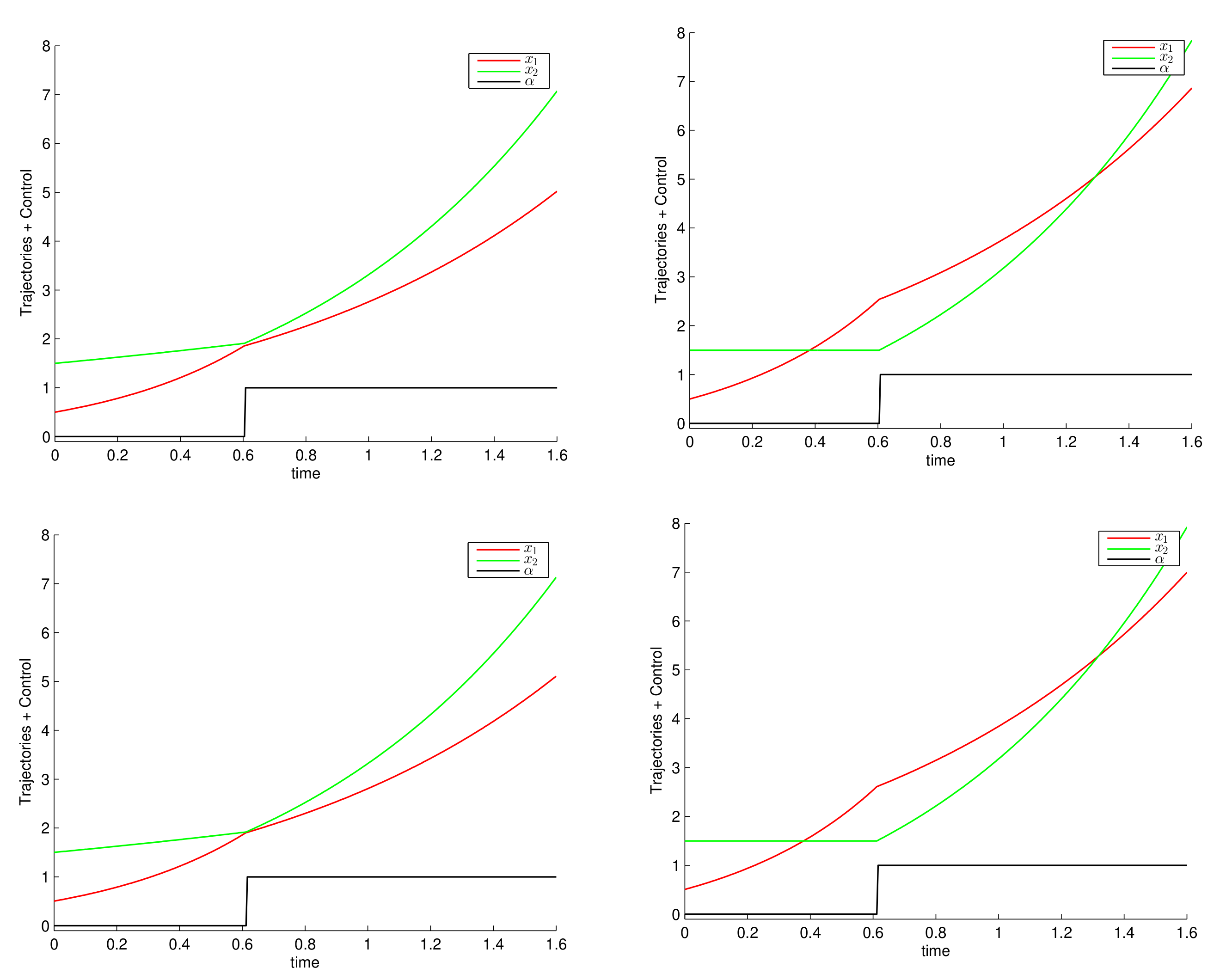
6.1. Constant Growth Rates

Let us consider system (5) where the growth rate functions follow Assumption 4 (constant values) with values given in

Table 1. Numerical values of the different parameters: case of constant growth rates.

${\mathit{a}}_1$	${\mathit{a}}_2$	${\mathit{r}}_1$	${\mathit{r}}_2$	${\mathit{Y}}_1$	${\mathit{Y}}_2$	T
2	1/2	1	0.1–0.5	1	1	2

.

In this case, the switching time $\overline{\tau }$ introduced by Equation (17) is given by $\overline{\tau }=log\left(4\right)$ and the optimal control is given by:

$${\alpha }^{☆}\left(t\right)=\left\{\begin{array}{cc}1\hfill & ift\ge min(0,2-log(4\left)\right)\hfill \\ 0\hfill & otherwise.\hfill \end{array}\right.$$

As underlined in Remark 2, the optimal control ${\alpha }^{☆}$ does not depend on the migration rate constant $r_2$. On Figure 2, we plot (with Matlab) the optimal control given by Proposition 3 together with the optimal trajectories in the two cases $r_2=0.1$ (bottom left) and $r_2=0.5$ (bottom right). As a verification, these plots are also compared with the ones obtained with Bocop [23], which is a numerical optimization software dedicated to optimal control problems (using direct method) on Figure 2 (top).

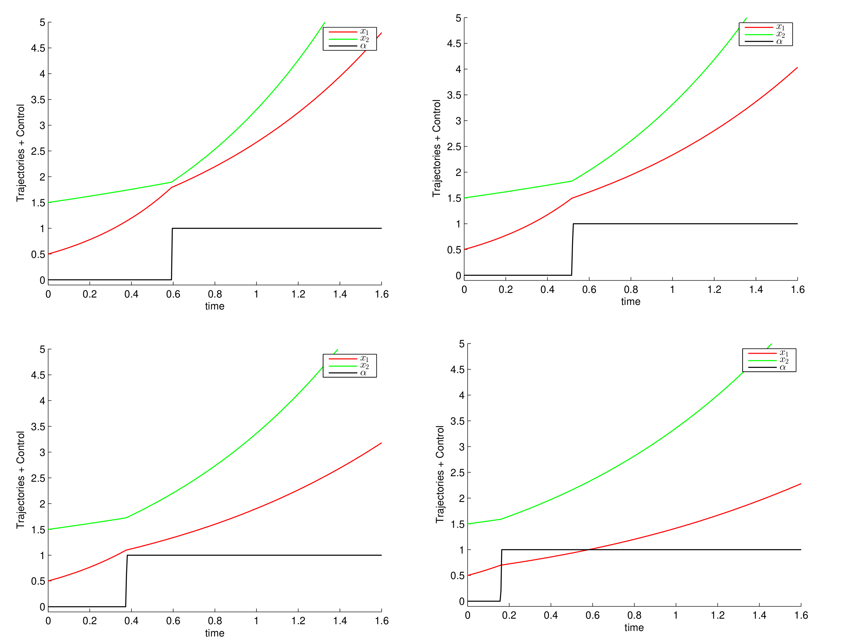
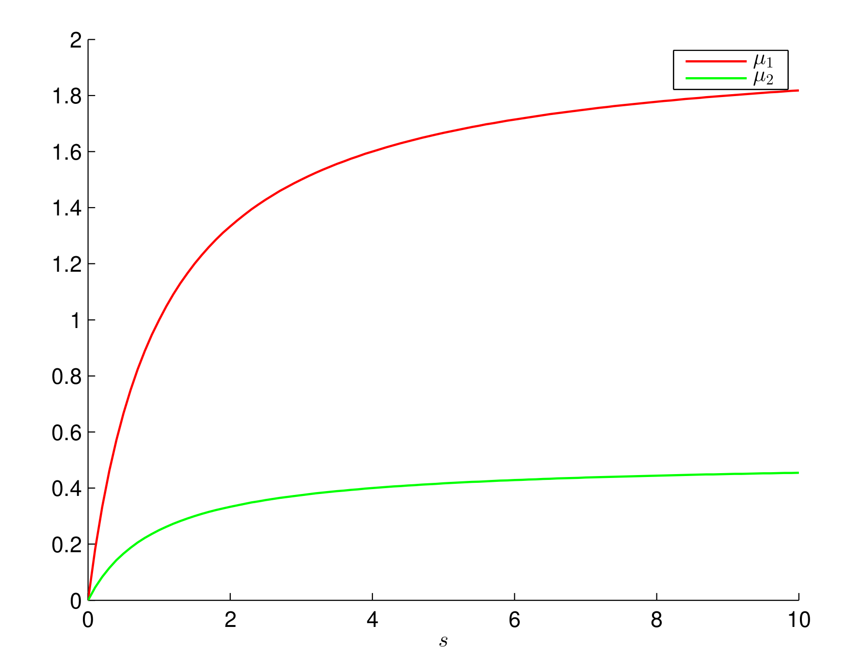
6.2. Monod Growth Rates

In this section, we consider system (5) with variable growth rate functions instead of constants ones, using the Monod expression (3).

Using the numerical solver Bocop, we simulate the optimal control together with the optimal trajectories in similar conditions than before with model parameters given in

Table 2. Numerical values of the different parameters: case of Monod-type growth rates (3).

${\mathit{k}}_1$	${\mathit{k}}_2$	${\mathit{K}}_{{\mathit{s}}_1}$	${\mathit{K}}_{{\mathit{s}}_2}$	${\mathit{r}}_1$	${\mathit{r}}_2$	${\mathit{Y}}_1$	${\mathit{Y}}_2$	T
2	1/2	1	1	1	0.1	1	1	2

, and for different values of initial control $c=s\left(0\right)+x_1\left(0\right)+x_2\left(0\right)$. Observe that, in this example, the growth kinetic functions ${\mu }_1$ and ${\mu }_2$ satisfy Assumption 3. Thus, thanks to Proposition 1, no singular arcs are present in this case. We observe in Figure 3 that the optimal trajectories have the same structure than for constant growth rates given by Proposition 3, however here the optimal switching time depends on the initial condition.

6.3. Consequences for the Control of Electro-Fermentation Experiments

We have proposed a model describing the effect of electro-fermentation on the metabolic profile of a fermentative bacteria in a batch culture. Fermentation and electro-fermentation behaviors $(f_1,f_2)$ each give rise to different products ($s_1,s_2$). The switching between the fermentation behaviors depends on the electrode potential V. As shown in Proposition 2, the optimal control strategy is trivial in the case where the electro-fermentation $f_2$ growth rate is higher or equal to the fermentation $f_1$ growth rate $(a_2\ge a_1)$. This indicates that in some experimental configurations, a dynamic control is not necessary to optimize the system. For example, in the case of Clostridium autoethanogenum electro-fermentation with [Co(trans-diammac)]³⁺ as the mediator reported by Kracke et al. [13], the electro-fermentation led to a 35-fold increase in lactate production, however the growth rate was not significantly impacted. In that case, the optimization of lactate production is straightforward and requires a constant polarization of the electrode at the electro-fermentation potential (−603 mV vs. standard hydrogen electrode). However, in other cases, the electro-fermentation growth rate is lower than the fermentation growth rate $(a_2<a_1)$. In such cases, the dynamic control strategy proposed in Proposition 3 would be required to optimize the production of the targeted product. This is the case, for example, for the electro-fermentation of glucose by Clostridium pasteurianum reported by Choi et al. [12]. In that case, they reported a 2.4-fold increase of butanol production associated with a 1.6-fold decrease in growth rate. Using values estimated in their experiments $a_1=$ $0.41$/$\mathrm{h}$ and $a_2=$ $0.25$/$\mathrm{h}$, and assuming a relatively high transition rate $r_1=$ 1/$\mathrm{h}$, the switching time $\overline{\tau }$ is then calculated using Equation (17): $\overline{\tau }\approx$ 5 $\mathrm{h}$. This means that the optimal production of butanol would then be obtained with a first period of fermentation without polarization of the electrode followed by 5 $\mathrm{h}$ of electro-fermentation. In the experiment reported by Choi et al. [12], according to Figure 4, the fermentation starts after a 15 $\mathrm{h}$ lag phase and ends around 23 $\mathrm{h}$. The optimal control would then correspond to polarizing the electrode at +45 mV vs. standard hydrogen electrode after 18 $\mathrm{h}$. This calculation also shows that the estimation of the true value of the transition rate $r_1$ would be crucial for such a control approach.

7. Conclusions and Perspectives

We propose a model describing the metabolic switching holding in an electro- fermentation process within a pure batch culture. Based on this model, an optimal control problem is formulated in order to maximize the production of one of the rising fermentation products. The Pontryagin’s Maximum Principle is applied for the analysis of the optimization problem. A preliminary result analyzing the behavior of the optimal control in the case of proportional growth functions is given. An optimal control is synthesized in two particular cases: similar and constant (but different) growth rate kinetics. The obtained results show that the optimal control strategy is far from being trivial, in the sense that undesirable metabolic pathways may be visited by the fermentative bacteria for the maximization of a desired fermentation product. Consequences of the obtained optimal strategy for driving electro-fermentation experiments are discussed through a realistic example. This study is elaborated under the hypothesis of identical yield factors.The optimality for the case of different yield factors with more general growth kinetics is an open problem that will be explored in the near future. This theoretical approach also underscores the importance of evaluating biological parameters such as transition rates between fermentation mode and electro-fermentation mode for the application of the optimal control. The proposed model as well as the optimal control law need to be confronted with experimental data, and this will be the subject of future experimental investigation within the LBE laboratory.

References

1. Logan, B.E.; Rabaey, K. Conversion of Wastes into Bioelectricity and Chemicals by Using Microbial Electrochemical Technologies. Science 2012, 337, 686–690. [Google Scholar] [CrossRef] [PubMed] [Green Version]
2. Rabaey, K.; Rozendal, R.A. Microbial electrosynthesis—Revisiting the electrical route for microbial production. Nat. Rev. Microbiol. 2010, 8, 706–716. [Google Scholar] [CrossRef] [PubMed]
3. Moscoviz, R.; Toledo-Alarcon, J.; Trably, E.; Bernet, N. Electro-Fermentation: How To Drive Fermentation Using Electrochemical Systems. Trends Biotechnol. 2016, 34, 856–865. [Google Scholar] [CrossRef] [PubMed]
4. Schievano, A.; Pepé Sciarria, T.; Vanbroekhoven, K.; De Wever, H.; Puig, S.; Andersen, S.J.; Rabaey, K.; Pant, D. Electro-Fermentation—Merging Electrochemistry with Fermentation in Industrial Applications. Trends Biotechnol. 2016, 34, 866–878. [Google Scholar] [CrossRef] [PubMed]
5. Zhou, M.; Freguia, S.; Dennis, P.G.; Keller, J.; Rabaey, K. Development of bioelectrocatalytic activity stimulates mixed-culture reduction of glycerol in a bioelectrochemical system. Microb. Biotechnol. 2015, 8, 483–489. [Google Scholar] [CrossRef] [PubMed]
6. Xafenias, N.; Anunobi, M.O.; Mapelli, V. Electrochemical startup increases 1,3-propanediol titers in mixed-culture glycerol fermentations. Process Biochem. 2015, 50, 1499–1508. [Google Scholar] [CrossRef] [Green Version]
7. Moscoviz, R.; Trably, E.; Bernet, N. Electro-fermentation triggering population selection in mixed-culture glycerol fermentation. Microb. Biotechnol. 2018, 11, 74–83. [Google Scholar] [CrossRef] [PubMed]
8. Toledo-Alarcón, J.; Moscoviz, R.; Trably, E.; Bernet, N. Glucose electro-fermentation as main driver for efficient H2-producing bacteria selection in mixed cultures. Int. J. Hydrog. Energy 2019, 44, 2230–2238. [Google Scholar] [CrossRef]
9. Paiano, P.; Premier, G.; Guwy, A.; Kaur, A.; Michie, I.; Majone, M.; Villano, M. Simplified Reactor Design for Mixed Culture-Based Electrofermentation toward Butyric Acid Production. Processes 2021, 9, 417. [Google Scholar] [CrossRef]
10. Emde, R.; Schink, B. Oxidation of glycerol, lactate, and propionate by Propionibacterium freudenreichii in a poised-potential amperometric culture system. Arch. Microbiol. 1990, 153, 506–512. [Google Scholar] [CrossRef] [Green Version]
11. Choi, O.; Um, Y.; Sang, B.I. Butyrate production enhancement by Clostridium tyrobutyricum using electron mediators and a cathodic electron donor. Biotechnol. Bioeng. 2012, 109, 2494–2502. [Google Scholar] [CrossRef] [PubMed]
12. Choi, O.; Kim, T.; Woo, H.M.; Um, Y. Electricity-driven metabolic shift through direct electron uptake by electroactive heterotroph Clostridiumpasteurianum. Sci. Rep. 2015, 4, 6961. [Google Scholar] [CrossRef] [PubMed]
13. Kracke, F.; Virdis, B.; Bernhardt, P.V.; Rabaey, K.; Krömer, J.O. Redox dependent metabolic shift in Clostridium autoethanogenum by extracellular electron supply. Biotechnol. Biofuels 2016, 9, 249. [Google Scholar] [CrossRef] [PubMed] [Green Version]
14. Kim, M.Y.; Kim, C.; Ainala, S.K.; Bae, H.; Jeon, B.H.; Park, S.; Kim, J.R. Metabolic shift of Klebsiella pneumoniae L17 by electrode-based electron transfer using glycerol in a microbial fuel cell. Bioelectrochemistry 2019, 125, 1–7. [Google Scholar] [CrossRef] [PubMed]
15. Engel, M.; Holtmann, D.; Ulber, R.; Tippkötter, N. Increased Biobutanol Production by Mediator-Less Electro-Fermentation. Biotechnol. J. 2019, 14, 1800514. [Google Scholar] [CrossRef] [PubMed]
16. Zhang, Y.; Li, J.; Meng, J.; Sun, K.; Yan, H. A neutral red mediated electro-fermentation system of Clostridium beijerinckii for effective co-production of butanol and hydrogen. Bioresour. Technol. 2021, 332, 125097. [Google Scholar] [CrossRef] [PubMed]
17. Harmand, J.; Lobry, C.; Rapaport, A.; Sari, T. Optimal Control in Bioprocesses: Pontryagin’s Maximum Principle in Practice; Chemical Engineering Series—Chemostat and Bioprocesses; Wiley: Hoboken, NJ, USA, 2019; Volume 3, p. 244. [Google Scholar]
18. Smith, H.; Waltman, P. The Theory of the Chemostat: Dynamics of Microbial Competition; Cambridge University Press: Cambridge, UK, 1995. [Google Scholar]
19. Pontryagin, L.; Boltyanski, V.; Gamkrelidze, R.; Michtchenko, E. The Mathematical Theory of Optimal Processes; The Macmillan Company: New York, NY, USA, 1964. [Google Scholar]
20. Haidar, I.; Rapaport, A.; Gérard, F. Effects of spatial structure and diffusion on the performances of the chemostat. Math. Biosci. Eng. 2011, 8, 953–971. [Google Scholar] [CrossRef] [PubMed]
21. Lee, E.B.; Markus, L. Foundations of Optimal Control Theory; John Wiley: Hoboken, NJ, USA, 1967. [Google Scholar]
22. Zelikin, M.I.; Borisov, V.F. Theory of Chattering Control: With Applications to Astronautics, Robotics, Economics, and Engineering; Systems & Control: Foundations & Applications; Birkhaüser: Basel, Switzerland, 1994. [Google Scholar]
23. Bonnans, F.; Martinon, P.; Giorgi, D.; Grélard, V.; Maindrault, S.; Tissot, O.; Liu, J. BOCOP 2.0. 5—User Guide. 2017, p. 480. Available online: http://bocop.org (accessed on 28 January 2022).
Figure 1. Scheme of the switching between the fermentation behaviors of a fermentative bacteria depending on the electrode potential V.
Processes 10 00535 g001
Figure 2. Exact optimal control (top) and optimal control computed with Bocop (bottom) for r 2 = 0.1 (left) and r 2 = 0.5 (right).
Processes 10 00535 g002
Figure 3. Optimal control computed with Bocop for c = 100 (top left), c = 30 (top right), c = 20 (bottom left), and c = 15 (bottom right).
Processes 10 00535 g003
Figure 4. Kinetic growth rates of the Monod type.
Processes 10 00535 g004