Prediction of Heavy Metal Concentrations in Contaminated Sites from Portable X-ray Fluorescence Spectrometer Data Using Machine Learning

Abstract

Portable X-ray fluorescence (pXRF) spectrometers provide simple, rapid, nondestructive, and cost-effective analysis of the metal contents in soils. The current method for improving pXRF measurement accuracy is soil sample preparation, which inevitably consumes significant amounts of time. To eliminate the influence of sample preparation on PXRF measurements, this study evaluates the performance of pXRF measurements in the prediction of eight heavy metals’ contents through machine learning algorithm linear regression (LR) and multivariate adaptive regression spline (MARS) models. Soil samples were collected from five industrial sites and separated into high-value and low-value datasets with pXRF measurements above or below the background values. The results showed that for Cu and Cr, the MARS models were better than the LR models at prediction (the MARS-R² values were 0.88 and 0.78; the MARS-RPD values were 2.89 and 2.11). For the pXRF low-value dataset, the multivariate MARS models improved the pXRF measurement accuracy, with the R² values improved from 0.032 to 0.39 and the RPD values increased by 0.02 to 0.37. For the pXRF high-value dataset, the univariate MARS models predicted the content of Cu and Cr with less calculation. Our study reveals that machine learning methods can better predict the Cu and Cr of large samples from multiple contaminated sites.

1. Introduction

Heavy metals are indestructible and non-biodegradable. They can occur in living organisms through biomagnification and bioaccumulation and present in high amounts in the environment, which leads to potential risks for human health and the environment [1,2,3,4]. Heavy metals can cause adverse effects on humans through the inhalation of respirable dust particles, the ingestion of foods from living organisms exposed to heavy metals, and dermal absorption [1,2,3,4].

Portable X-ray fluorescence (pXRF) spectrometers can provide simple, rapid, nondestructive, and cost-effective analysis of the metal contents in soils and have been widely used to assess environmental risks, predict soil properties, and evaluate soil fertility, among other uses [5,6,7,8,9]. According to the Chinese Standard Technical Guidelines for the Investigation on Soil Contamination of Land for Construction [10], the heavy metal rapid detector is recommended for the qualitative and quantitative analysis of heavy metals in soils in situ. The pXRF instrument can help to guide the selection of samples to be analyzed in the laboratory and make investigative and remediative decisions [11,12].

The pXRF instrument realizes the qualitative and quantitative analysis of soil properties through X-ray fluorescence intensities. Normally, X-ray fluorescence intensities are used to evaluate elemental concentrations, mostly using fundamental parameters (FP), empirical coefficients methods, or Compton peak ratios [13], based on the assumptions of sample homogeneity, plain surface, negligible particle size effects, and a priori knowledge of the sample matrix composition [14]. Therefore, some factors, such as physical matrix effects (e.g.,: particle size, homogeneity, surface conditions), moisture content, and chemical matrix effects (e.g.: the presence of iron reduces Cu but enhances Cr measurements) influence the accuracy of the measurements [13,15]. The current method for improving pXRF measurement accuracy is the preparation of soil samples, including screening, grinding, drying, etc. [13,16,17,18]. Method 6200 [13] recommends that for the obtainment of high-quality data, samples should be dried for 2 to 4 h in a convection or toaster oven at a temperature not greater than 150 °C, and then ground with a mortar and pestle and passed through a 60-mesh sieve to achieve a uniform particle size. Sample grinding should continue until at least 90 percent of the original sample passes through the sieve.

In practice, in most site investigations, the pXRF instrument directly measures heavy metal contents without sample preparation. To eliminate the influence of sample preparation on pXRF measurements, models have been used to correct pXRF measurements through the correlation between pXRF measurements and laboratory concentrations. Linear regression (LR) models are commonly used to evaluate the accuracy of pXRF measurements [12,16,17]. Caporale et al. defined metal-based linear models predicting laboratory concentrations from pXRF measurements for two case studies (agricultural and industrial sites) [19]. Their linear regressions revealed strong variability among their studied metals, providing good correlations only for Cu, Pb, and Zn at both sites [19]. For most of the metals, each metal-regression line significantly differed between the two case studies, indicating the site-dependence of the regression fits [19]. Chen et al. built a general modeling method and process based on the relationship between pXRF measurements and site parameters (organic matter and water content) to construct pXRF correction models, which could improve each site’s measurement accuracy [20]. The error in heavy metal pXRF measurements decreased from 22.9–75.7% to 9.6–26.9% and showed that models can be used to improve pXRF measurements for Pb, Zn, Fe, and Mn [20]. The results also indicated it is difficult to develop a model that is suitable for every site, because of the particularity of different sites [20]. In addition to site-specific models, some models were built on a large scale. Adler et al. adopted the machine learning method multiple linear regression (MLR), multivariate adaptive regression spline (MARS), and random forest (RF) to create national prediction models for Cu, Zn, and Cd concentrations in agricultural soil [21]. Predictive models using pXRF measurements were created and found to be applicable at the farm and national scales, and the results showed that the MLR model had good performance for predicting Zn, while the MARS model had better performance in the prediction of Cu and Cd in small-scale farmland [21].

In general, although sample preparations could improve pXRF measurement accuracy, they inevitably consume significant amounts of time and preclude the rapid selection of samples to be analyzed in the laboratory. Models have been used to correct pXRF measurements, but they were mainly site-specific models. Studies of predictive models for multiple industrial sites are still limited. Machine learning methods were successfully used in national agricultural soils in Sweden [21]. However, unlike agricultural soils, large variability in the spatial distribution and content of metals is generally recognized in the anthropogenically polluted soils of industrial sites [22]. Therefore, machine learning methods, including LR and non-linear MARS models, were explored to predict eight heavy metals (Cr, Ni, Cu, Zn, As, Cd, Hg, and Pb) in soil samples from five industrial sites. Laboratory concentrations were used to evaluate the predictive performance. In this study, the objectives were to (a) build prediction models of each heavy metal for samples from multiple industrial sites, (b) compare the performance of LR and MARS models for each heavy metal, and (c) examine the models’ performance when predicting heavy metals above or below the natural background values (BVs).

2. Materials and Methods

2.1. Soil Sampling and pXRF Rapid Measurement

The study is based on five site investigations; the industrial sites were formerly used as fertilizer factories, pesticide factories, or steel plants. Soil samples were collected according to the standard of Technical Specification for Soil Environmental Monitoring [23] and, subsequently, the pXRF was used to analyze the contents of heavy metals. After removing the gravel and other debris in soil samples, samples were put into transparent polyvinyl chloride (PVC) plastic bags, tamped, and flattened to ensure their thicknesses were at least 15 mm; they were then tested by pXRF in soil mode for at least 60 s.

In this study, the pXRF instruments included Explorer 9000 (Jiangsu Skyray Instrument Co., Ltd., Kunshan, China), X-MET7000 (Oxford Instruments, Shanghai, China), VANTA-VLW (Olympus, Center Valley, PA, USA), DP-4050 (Olympus, Center Valley, PA, USA), and VANTA-VCA (Olympus, Center Valley, PA, USA). The pXRF instrument used in each site was different; total five types of pXRF instrument were used, and the limits of detection for each heavy metal are shown in

Table 1. Limits of detection (LODs) of each pXRF instrument (mg/kg).

Metals	Explore 9000	X-MET7000	VANTA-VLW	DP-4050	VANTA-VCA
Cr	7.68	5	20	4–10	20
Ni	4.65	5	20	5–15	4
Cu	8.5	5	20	4–8	3
Zn	1.8	5	5	1–3	2
As	3.6	5	3	1–3	1
Cd	2.2	5	10	2–3	5
Hg	0.8	5	9	1–4	2
Pb	2.5	5	1	2–4	3

. All operators were well trained, and the procedure followed the manufacturer’s instructions and the recommendations of Method 6200 [13]. Therefore, the influences of pXRF instruments were neglected and not discussed.

2.2. Laboratory Analyses

Soil samples were sent to laboratories to analyze Cr, Cu, Pb, As, Ni, Cd, Zn, and Hg concentrations. The analytical methods of each heavy metal are shown in Supplementary Table S1. The soil samples were air-dried, ground, and passed through a 100-mesh sieve, and then Cr, Ni, Cu, Zn, Cd, and Pb in soil samples were extracted by HCl-HNO₃-HF-HClO₄ electric heating plate digestion. The Hg and As were extracted by aqua regia water bath digestion.

2.3. Data Preprocessing Method

Before performing the regression analysis, outliers were removed based on the box-and-whiskers plot [24] and calculated in Python 3.7, according to the following upstream criteria:

(a)

undetected (NA) data in the pXRF measured data or laboratory analyzed data of soil samples were removed;

(b)

calculate for each variable (metal) the ratio (X)_XRF/(X)_LAB, where (X)_XRF is the metal concentration obtained by pXRF and (X)_LAB by laboratory analysis;

(c)

calculate the first quartile (Q₁) and third quartile (Q₃) of these ratios;

(d)

outliers were the ratios greater than Q₃ + 1.5 × (Q₃ − Q₁) or lower than Q₁ − 1.5 × (Q₃ − Q₁), and then were deleted from datasets.

2.4. Statistical Method

Descriptive statistics (including mean, standard deviation, and coefficient of variation) were calculated in Python 3.7.

Pearson correlation coefficients between the pXRF measurements and the laboratory concentrations were calculated in SPSS 20.0.0. The Pearson correlation indicates the linearity between two parameters, and it is generally believed that the coefficient between 0.8–1.0 shows a highly related correlation; 0.6–0.8 shows a strong related correlation; 0.4–0.6 indicates a moderate related correlation; 0.2–0.4 shows a weak related correlation; and 0.0–0.2 shows a very weak related correlation or no related correlation [25].

The geo-accumulation index (I_geo) is widely used to estimate the magnitude of anthropogenic activities [19]. I_geo was originally proposed by Müller [26] and can be calculated as follows:

$$I_{geo}={\log }_2\left(\frac{C_n}{1.5B_n}\right)$$

(1)

where C_n is the metal content determined by laboratory (mg/kg) and B_n is the background concentration (mg/kg); 1.5 was considered as natural fluctuations due to a very small anthropogenic influence. According to Müller [27], categories based on I_geo were established as follows: unpolluted (I_geo ≤ 0), unpolluted-to-moderately-polluted (0 < I_geo ≤ 1), moderately polluted (1 < I_geo ≤ 2), moderately-to-heavily-polluted (2 < I_geo ≤ 3), heavily polluted (3 < I_geo ≤ 4), heavily-to-extremely-polluted (4 < I_geo ≤ 5), and extremely polluted (I_geo > 5).

2.5. Prediction Model

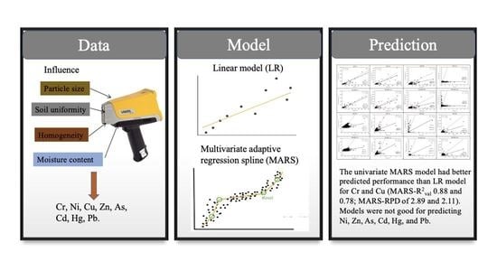
2.5.1. Model Introduction

Linear Regression

As one of the most basic machine learning methods, the LR model is widely used in various fields. The linear regression model is a statistical analysis method and used to determine the quantitative relationship between two or more variables in regression analysis. The optimal parameters of the model are calculated by the least square method.

Multivariate Adaptive Regression Spline Model

The MARS model is a spline regression method that can adaptively process high-dimensional data; it was proposed by the statistician Jerome Friedman in 1991 [28]. It is a nonparametric statistical method based on a divide-and-conquer strategy in which the training data sets are partitioned into separate piecewise linear segments (splines) of differing gradients (slope). MARS makes no assumptions about the underlying functional relationships between dependent and independent variables. In general, the splines are connected smoothly together, and these piecewise curves (polynomials), also known as basis functions, result in a flexible model that can handle both linear and nonlinear behavior [29,30].

Univariate and Multivariate Models

In this study, univariate LR and MARS and multivariate MARS models were adopted. The univariate model used pXRF measurements of one heavy metal as the predictor and realized prediction of its corresponding heavy metal content in soil samples. By contrast, the multivariate model used pXRF measurements of eight heavy metals as the predictors. The MARS model was used to build the multivariate model, since it allowed missing values in the predictors while the LR model did not.

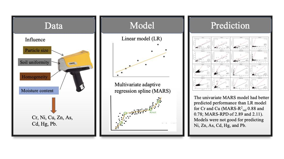
2.5.2. Model Prediction and Validation Process

The model process is presented in Figure 1. Leave-one-out cross-validation (LOOCV) was adopted to evaluate the model’s performance [7,31]. If the size of the dataset was N, then N-1 pieces of data were used for training, and the remaining pieces were used for validation. Each time, one datum was used as validation until all samples were validated, at which point, a total of N times was calculated. LOOCV is suitable for small datasets and can prevent over-fitting and evaluate the model’s generalization ability.

The linear model was in Scikit-learn 0.22.1 from Python 3.7, and the MARS model was from Py-earth 0.1.0. The LOOCV was from LeaveOneOut in Scikit-learn 0.22.1.

2.5.3. Model Evaluation

Three parameters evaluated the predictive accuracy of the model: the determination coefficient (R²), the prediction of the root mean squared error (RMSE), and the ratio of percent deviation (RPD). The value of R² reflected the stability of the model establishment and verification. The closer the R² value to 1, the better the model. If the R² value was more significant than 0.7, it was generally considered that the model was good [32]. The smaller the RMSE, the more stable the model’s performance. RPD was the ratio of the standard deviation of the validation data to the RMSE of the predictive result, which could be used to judge the model’s predictive ability. When RPD < 1.4, the model could not realize prediction; when 1.4 ≤ RPD < 2.0, the model had regular predictive performance and could be used to perform rough predictions; when RPD ≥ 2.0, the model had excellent predictive ability [33].

3. Results

3.1. Descriptive Statistics of pXRF-Measured Data and Laboratory-Analyzed Data

The descriptive statistics and coefficients of variations (CVs) of the pXRF measurement and laboratory concentration of each heavy metal are presented in

Table 2. Statistical characteristics of pXRF and laboratory-analyzed results (mg/kg).

Heavy Metal	pXRF-Cr	pXRF-Ni	pXRF-Cu	pXRF-Zn	pXRF-As	pXRF-Cd	pXRF-Hg	pXRF-Pb
Counts	1363	2108	2232	1607	2721	1105	546	2502
Mean	102.95	23.59	47.18	82.30	10.81	2.31	0.38	27.20
Std	429.14	15.26	266.02	119.42	9.56	2.58	1.46	34.89
Min	2.07	0.46	0.25	1.77	0.030	0.00030	0.00050	0.034
25%	41	15	17	53.87	5	0.28	0.021	14.11
50%	56.06	20.98	24	66	8	1	0.045	21
75%	75.71	28	32	80.84	15	4	0.091	27
Max	10845	232.14	7905	3044	201.58	13	25.62	670.80
CV	4.17	0.65	5.64	1.45	0.88	1.12	3.82	1.28
Heavy Metal	Lab-Cr	Lab-Ni	Lab-Cu	Lab-Zn	Lab-As	Lab-Cd	Lab-Hg	Lab-Pb
Counts	1363	2108	2232	1607	2721	1105	546	2502
Mean	121.61	32.83	57.93	125.21	11.87	0.11	0.13	36.14
Std	365.00	10.60	242.94	262.44	7.38	0.15	0.66	59.73
Min	13.93	4.21	4	29	1.01	0.010	0.0030	7.30
25%	53.50	24.50	22	55	8.60	0.060	0.016	20
50%	68	33.50	28	66	10.80	0.090	0.027	24
75%	89	40	35	83	13.90	0.12	0.062	29.90
Max	7400	168.55	5000	5720	196.27	3.08	13.26	1380
CV	3.00	0.32	4.19	2.10	0.62	1.30	4.90	1.65

. The heavy metals As, Pb, and Cu had large sample sizes (2721, 2502, and 2232, respectively). The average concentrations of Cr, Ni, Cu, Zn, As, Cd, Hg, and Pb measured by pXRF were 102.95, 23.59, 47.18, 82.30, 10.81, 2.31, 0.38, and 27.20 mg/kg, respectively, which were smaller than the average laboratory concentrations of 121.61, 32.83, 57.93, 125.21, 11.87, 0.11, 0.13, and 36.14 mg/kg, respectively.

The CVs of the pXRF measurements were comparable to those of the laboratory concentration of each heavy metal. The CVs of the pXRF measurements and laboratory concentrations of Cr, Cu, Zn, Cd, Hg, and Pb were greater than 1, which indicated higher variation, and that these heavy metals were greatly affected by anthropogenic influences [31]. Apart from Cd, no significant difference in metal concentration between the pXRF-measured data and the laboratory-measured data was observed for other metals, indicating that in situ pXRF can be reliably used to investigate the concentrations of heavy metals. For Cd, the statistical characteristics of the concentrations between the pXRF-measured data and the laboratory-measured data were different. These results may be explained by the low detection limits of the pXRF instrument (2 mg/kg).

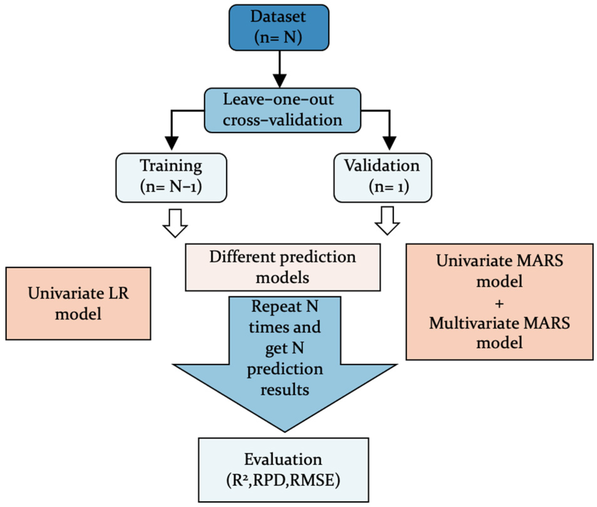
3.2. Univariate LR and MARS Model Predictive Results

Predictive Results of Soil Samples from the Whole pXRF-Measured Dataset

The pXRF measurements of each heavy metal were used to predict the contents analyzed in the laboratory through the univariate LR and MARS model, according to the modeling process in Section 2.5.2. The predicted contents against the laboratory concentrations are shown in Figure 2.

The R² and RPD values of the MARS models for predicting Cr (0.88, 2.89) and Cu (0.77, 2.11) were larger than those of the LR models for Cr (0.8, 2.22) and Cu (0.73, 1.94), which indicated that the MARS models were better than the LR models at predicting Cu and Cr. For the other six heavy metals, the R² values of the LR and MARS models were smaller than 0.7, and their RPD values were smaller than 1.4, indicating that the LR and MARS models could not be used for predicting them. The fitness of the LR model for predicting Cr and Cu, and that of the MARS model for predicting Cu, were consistent with other research [12,20,21].

Considering the need to accurately select high concentrations of heavy metal samples to be analyzed in the laboratory and the fact that contaminated industrial sites were primarily impacted by human activities, the first level in the Environmental Quality Standards for Soils [34] was used as the BV to divide the pXRF dataset into two parts (

Table 3. Natural background value of each heavy metal and the concentration range of the two datasets.

Heavy Metal	BVs (mg/kg)	pXRF Low-Value Dataset			pXRF High-Value Dataset
		Sample Size	pXRF Range (mg/kg)	Lab Range (mg/kg)	Sample Size	pXRF Range (mg/kg)	Lab Range (mg/kg)
Cr	90	1144	2.08–89.05	13.93–337	219	90.01–10845	48–7400
Ni	40	1949	0.47–39.86	4.21–104	159	40.51–106	20–74
Cu	35	1843	0.25–34.84	4–1350	389	35.08–7905	17–5000
Zn	100	1367	1.78–99.56	29–1680	240	100.61–3044	56–5720
As	15	2071	0.038–14.84	1.01–86.30	650	15.01–201.58	5.85–196.27
Cd	0.2	151	0.00030–0.20	0.010–0.76	954	0.20–13.00	0.017–3.09
Hg	0.15	456	0.00050–0.15	0.0030–5.99	90	0.15–25.62	0.011–13.27
Pb	35	2202	0.034–34.78	7.30–1040	300	35.56–670.80	20–1380

). The samples of pXRF measurements larger than the BV were classified into the pXRF high-value dataset, and the samples of the pXRF measurements that were lower than the BV were classified into the pXRF low-value dataset. Their corresponding laboratory-analyzed data were also divided into two datasets. The detailed statistical characteristics of the pXRF low-value and high-value datasets are shown in Supplementary Tables S2 and S3. The models were trained to predict heavy metal concentrations for samples in the pXRF high-value and the pXRF low-value datasets separately, and the predicted results are presented in Figure 3 and Figure 4.

The results of the pXRF low-value dataset showed that the R² and RPD values of the LR and MARS models were smaller than 0.1 and 1.4, which indicated that the models could not predict the concentrations of each heavy metal through the pXRF measurements (Figure 3).

For the pXRF high-value dataset (Figure 4), the R² and RPD values of the MARS models for predicting Cr (0.88, 2.84) and Cu (0.79, 2.18) were larger than those of the LR models for Cr (0.8, 2.22) and Cu (0.75, 2.00), which indicated that the MARS models were better than the LR models at predicting Cu and Cr. However, neither the LR model nor the MARS model were suitable for predicting the concentrations of the other six heavy metals for the samples in the pXRF high-value dataset.

In Figure 4a,b,i,j, when the laboratory concentrations of Cu and Cr were smaller than 2000 mg/kg, the LR model had more accurate predictive results than the MARS model, since the black points in the LR model were closer to the 1:1 line (the closer the points were to the 1:1 line, the more the predicted results equaled to the lab concentrations). When the laboratory concentrations were greater than 2000 mg/kg, the MARS model had more accurate predictive results than the LR model, and the predicted points were closer to the 1:1 line in the MARS model than in the LR model. The same results were also found for the samples from the whole dataset when predicting Cu and Cr (Figure 2).

3.3. Multivariate MARS Model Predictive Results

3.3.1. Predictive Results of Samples in the pXRF Low-Value Dataset

Unlike the univariate MARS model, which used the pXRF measurement of one heavy metal as the predictor, the multivariate MARS model used the pXRF measurements of other seven heavy metals as the predictors. We explored whether the increase in the predictors could improve the predicted results. The results of the multivariate MARS models for predicting the contents of Cr, Cu, Pb, As, Ni, Cd, Zn, and Hg in the samples from the pXRF low-value dataset are shown in

Table 4. Validation statistics for predictive results of heavy metals of sample in the pXRF low-value dataset and Cr and Cu of sample in pXRF high-value dataset using univariate and multivariate MARS model.

Heavy Metals	Univariate MARS			Multivariate MARS
	R2	RMSE	RPD	R2	RMSE	RPD
pXRF Low-Value Dataset
Cu	0.12	10.84	1.06	0.51	8.04	1.43
Cr	0.12	23.05	1.07	0.44	18.32	1.34
Ni	0.14	9.32	1.08	0.44	7.53	1.34
As	0.13	3.91	1.07	0.32	3.47	1.21
Pb	0.12	6.96	1.07	0.23	6.51	1.14
Hg	−0.0044	0.03	1.00	0.14	0.034	1.08
Zn	0.098	14.07	1.05	0.13	13.85	1.07
Cd	−0.013	0.06	1.00	−0.35	0.063	0.86
pXRF High-Value Dataset
Cr	0.87	306.14	2.80	0.88	294.28	2.92
Cu	0.79	255.50	2.18	0.71	301.34	1.84

.

Comparing the results between the univariate MARS and multivariate MARS models, the R² values improved from 0.032 to 0.39, the RPD values increased by 0.02 to 0.37, and the RMSE decreased by 0.22 to 4.73. The results showed that the predictive performance of the multivariate MARS models significantly improved for the heavy metals, except for Cd.

The multivariate MARS model had the best predictive ability for Cu (R² and RPD values were 0.51, 1.43, respectively). Compared with the univariate predictive result of Cu (R² and RPD values were 0.12, 1.06, respectively), the R² and RPD values of the multivariate MARS model increased by 0.39 and 0.37. However, for the other heavy metals, the RPD values were less than 1.4, indicating that the predictive abilities of the multivariate models for the other heavy metals were still limited.

3.3.2. Predictive Results of Samples in the pXRF High-Value Dataset

Given that the results that the predictive performance of the univariate MARS model for the Cr and Cu in the samples from the pXRF high-value dataset were good, Cr and Cu were selected to be predicted by the multivariate MARS models, and the results are presented in Table 4. The results showed that the predicted abilities of the univariate and multivariate MARS model for Cr were similar (the R² and RPD values were 0.87 and 2.80 and 0.88 and 2.92, respectively). For Cu, the univariate MARS model was better than the multivariate MARS model at prediction (the R² and RPD values were 0.79, 2.18, and 0.71, 1.84, respectively).

Overall, the multivariate MARS model was a slight improvement on the predictive performance for Cr and Cu of the univariate MARS model.

4. Discussion

4.1. Influences of pXRF’s Accuracy on Model’s Predictive Results

The high accuracy of the pXRF instrument when measuring heavy metals resulted in strong linearity between the pXRF measurements and laboratory concentrations. For the univariate models, the linear correlations between the PXRF measurements and laboratory concentrations were related to the predicted performance of the models, especially the LR models. This study predicted Cu and Cr from corresponding pXRF measurements, while the models could not predict the other heavy metals. The Pearson correlation coefficients showed the linearity between the pXRF measurements and the corresponding laboratory concentrations, which were 0.9 and 0.88 for Cu and Cr, respectively (Figure 5). The coefficients of Cu and Cr were larger than those of the other heavy metals, which were smaller than 0.8 (Figure 5) and could explain the excellent predictive performance of the models.

The accuracy of the pXRF instrument for different heavy metals was not universal. The excellent linearity between the pXRF measurement and the laboratory concentrations of Cu coincided with the research of Kilbride et al. and Potts et al. [12,35]. Kilbride et al. measured Cu with a range from 3 to 5140 mg/kg, which was a similar range to that used in the current study (4–5000 mg/kg), and found a good accuracy of pXRF for Cu [12]. Potts et al. found that pXRF was not sufficiently sensitive for the determination of Cu with concatenations lower than 200 mg/kg [35]. Therefore, a wide range of Cu in our study could be accurately measured by pXRF. Some research also found a strong linear correlation between PXRF measurement and laboratory concentrations of As [12,16], while the results for As in the present study did not echo those of previous studies. Tian et al. found a weak correlation between the pXRF and laboratory data of As that might have been attributable to the narrow range of concentrations [36]. The range of As in our research was relatively narrow compared with those of Cu or Cr, which might be the reason for the poor linearity of As compared to Cu and Cr. Another reason through which to explain the poor linearity of As might be the presence of Pb. Some research indicated that the presence of high concentrations of Pb could compromise the pXRF’s precision for As [37,38], since Pb and As x-rays would cause spectral interferences and impact each other during measurement [13].

The low Pearson coefficients of Ni and Cd (0.37, 0.07) indicated the poor accuracy of pXRF for Ni and Cd, which was also found by Kilbride et al. (2006). For Hg, most soil samples (75%) had laboratory concentrations smaller than 0.1 mg/kg (Table 2), which were below the pXRF detection limit of 0.8 mg/kg (Table 1). Similarly, as with Cd, more than 75% of the samples had laboratory concentrations below the pXRF detection limit of 2.2 mg/kg (Table 1 and Table 2). Therefore, poor accuracy of pXRF was found for Hg and Cd [17].

4.2. Influences of Concentration on Model’s Predictive Results

Much research has confirmed that wider ranges of concentrations result in strong linearity between pXRF measurements and laboratory concentrations for Cu and Zn. The smaller the metal concentration in the soil sample, the higher the difference between the pXRF measurement and the laboratory concentration [36,39]. Li et al. also found that when the concentrations of Cu and Cr were greater than the first standard in the Environmental Quality Standards for Soils [34,40], which was used to separate the pXRF high-value and low-value datasets, the accuracy of the pXRF instrument was high. Therefore, high concentrations soil samples would result in better predictive model performance compared with low-concentration samples. The current study also confirmed the different predictive results between the pXRF high-value dataset and the pXRF low-value dataset. The R² and RPD univariate prediction model values for the samples from the pXRF high-value dataset were larger than those of the samples from the pXRF low-value dataset (Figure 3 and Figure 4).

Although the high-concentration samples had good predictive results, the univariate predictive results between the samples from the whole dataset and the pXRF high-value dataset were not significantly different. Although the sample size of the pXRF low-value dataset was larger than that of the pXRF high-value dataset, the low-concentration data had little influence on the prediction model. The high-concentration data, especially some abnormally high-concentration data, were found in contaminated sites and usually came from anthropologic activities. These data were minor but would enlarge the x-coordinate and cluster small-value data to exert a small influence on the predictive results. Thus, the univariate models made no obvious difference to the prediction of heavy metal contents from the samples from the pXRF high-value and whole datasets.

The results showed that the univariate models had a similar predicted ability for the samples from the pXRF high-value and whole datasets. Based on the need to investigate high-concentration data in site investigations, and the fact that the soil samples with concentrations above the BV were fewer than the soil samples with concentrations below the Bs, pXRF could help select high-concentration data (above BVs) to train the models with fewer calculations.

4.3. Comparation between LR and MARS Models

In this study, the MARS models showed less bias at high concentrations than the LR models (Figure 2 and Figure 4). Adler et al. also found the same result, that MARS models had the least negative bias when predicting Cu and Cd at higher concentrations compared to MLR and RF models [21]. The better predictive ability of the MARS model in high-concentration ranges may be explained by the accuracy of the pXRF instrument and the advantage of the MARS model as a nonlinear model. The higher the concentrations of heavy metals in samples, the more accurate pXRF instrument [36,39]. Therefore, it could be inferred that the linear relation between the pXRF-measured data and the laboratory-analyzed data from the heavy metals differed between high- and low-concentration samples. The linear relationship was stronger in the samples with high concentrations than it was in those with low concentrations; therefore, the MARS model could build different linear models at different concentration ranges. This could help explain why the MARS model could perform better than the LR model by creating more than one linear model for predicting the concentrations of Cu and Cr.

4.4. Comparison between Univariate and Multivariate Models

The multivariate MARS model was better than the univariate MARS model at predicting the heavy metal concentrations for the samples in the pXRF low-value dataset (Table 4). However this result was not strongly expressed in the samples in the pXRF high-value dataset (Table 4).

The soil samples from the pXRF low-value dataset had heavy metal contents measured by pXRF lower than the BV and were assumed not to have been interrupted by other pollution sources. The I_geo of each heavy metal sample was calculated from their laboratory concentrations and BVs, which indicated the magnitude of anthropogenic influences (Figure 6). For the pXRF low-value dataset, the I_geo results confirmed that these heavy metals were not polluted by human activities and came from the same natural source (Figure 6a). The pXRF measurements of the heavy that they received metals were below the BV, and the I_geo results for all the metals were negative, indicating no anthropogenic discharge contributions. Hence, the heavy metals in the samples from the pXRF low-value dataset came from the same natural source. According to the research about heavy metals’ source apportionment, heavy metals with similar sources are highly correlated [41,42,43]. The correlation of each heavy metal would contribute to the good predictive performance of multivariate models compared with the univariate model.

In the pXRF low-value dataset, the Pearson correlation coefficients between the pXRF measurements of Pb with laboratory concentrations of Cr and Cu were larger than 0.6 (Figure 7a), which was larger than the coefficients between the pXRF measurement with laboratory a concentration of Cr (0.35) and the pXRF measurement with a laboratory concentration of Cu (0.33). For Hg, the coefficient between the pXRF measurement of Cu and the laboratory concentration of Hg (0.57) was higher than the coefficient between the the pXRF measurement and the laboratory concentration of Hg (0.31). Therefore, adding the pXRF measurement of other heavy metals could improve the multivariate model’s performance.

In the pXRF high-value dataset, the samples had concentrations of heavy metal larger than the BV and were collected from different industry sites, which meant that these samples may have been polluted by different pollution sources. For the pXRF high-value dataset, a positive I_geo was observed for Cr, Cu, Zn, and Pb, and the I_geo for Zn was the largest, which showed moderate pollution (Figure 6b). The I_geo for Cr, Cu, and Pb showed unpolluted to moderately-polluted levels, and Ni, As, Cd, and Hg were observed with no anthropogenic influences. These results indicated that the pXRF instrument could roughly identify the anthropogenic pollution for Cr, Cu, Zn, and Pb. For Ni and As, the pXRF instrument performed poorly at identifying anthropogenic influences. For Cd and Hg, since most of them had concentrations below the detection limit, the pXRF results were not convincing. Caporale et al. found that the laboratory content was much closer to the content measured by pXRF when the source of the soil metal pollution was partially or completely from anthropogenic contamination [19]. This coincided with the finding in the current research that the coefficients between the pXRF measurements and the laboratory concentrations of Cu and Cr were larger than the other six heavy metals (Figure 7b). By contrast, Zn and Pb showed relatively low coefficients, which meant that the accuracy of pXRF at detecting them was poor compared to Cu and Cr (Figure 7b).

In the pXRF high-value dataset, the correlation coefficients between the pXRF measurements and the laboratory concentrations of Cr and Cu were the highest (Figure 7). There was no heavy metal with pXRF measurement significantly correlated to the laboratory concentrations of Cr and Cu. The different pollution sources explained why the correlated relationship between different heavy metals was not strong. Therefore, the pXRF measurement of other heavy metals was weekly correlated to the laboratory content of the heavy metal, and adding their pXRF measurements could hardly improve the model’s performance.

5. Conclusions

This study demonstrates that machine learning methods realized the prediction of Cu and Cr contents from pXRF measurements of soil samples from multiple contaminated sites. For Cu and Cr, the MARS model was better than the LR model at predicting the contents. The predicted results of samples in the pXRF high-value and pXRF low-value datasets showed that the univariate and multivariate MARS models performed well.

In general, the different predictive models could be chosen for different purposes. To obtain accurate predictions for high-concentration soil samples, high-concentration soil samples (pXRF measurements above BVs) were used to train the univariate MARS models with fewer calculations. To obtain accurate predictions for low-concentrations soil samples, multivariate MARS models could be used.

References

1. Sobhanardakani, S. Potential health risk assessment of heavy metals via consumption of caviar of Persian sturgeon. Mar. Pollut. Bull. 2017, 123, 34–38. [Google Scholar] [CrossRef] [PubMed]
2. Sobhanardakani, S. Ecological and Human Health Risk Assessment of Heavy Metal Content of Atmospheric Dry Deposition, a Case Study: Kermanshah, Iran. Biol. Trace Elem. Res. 2019, 187, 602–610. [Google Scholar] [CrossRef] [PubMed]
3. Sobhanardakani, S.; Tayebi, L.; Hosseini, S.V. Health risk assessment of arsenic and heavy metals (Cd, Cu, Co, Pb, and Sn) through consumption of caviar of Acipenser persicus from Southern Caspian Sea. Environ. Sci. Pollut. Res. 2018, 25, 2664–2671. [Google Scholar] [CrossRef] [PubMed]
4. Sobhanardakani, S. Human Health Risk Assessment of Cd, Cu, Pb and Zn through Consumption of Raw and Pasteurized Cow’s Milk. Iran. J. Public Health 2018, 47, 1172–1180. [Google Scholar]
5. Weindorf, D.C.; Bakr, N.; Zhu, Y. Advances in Portable X-ray Fluorescence (PXRF) for Environmental, Pedological, and Agronomic Applications. In Advances in Agronomy; Sparks, D.L., Ed.; Academic Press: Newark, NJ, USA, 2014; Volume 128, Chapter 1; pp. 1–45. ISBN 9780128021392. [Google Scholar] [CrossRef]
6. Benedet, L.; Faria, W.M.; Silva, S.H.G.; Mancini, M.; Demattê, J.A.M.; Guilherme, L.R.G.; Curi, N. Soil texture prediction using portable X-ray fluorescence spectrometry and visible near-infrared diffuse reflectance spectroscopy. Geoderma 2020, 376, 114553. [Google Scholar] [CrossRef]
7. Wan, M.; Hu, W.; Qu, M.; Li, W.; Zhang, C.; Kang, J.; Hong, Y.; Chen, Y.; Huang, B. Rapid estimation of soil cation exchange capacity through sensor data fusion of portable XRF spectrometry and Vis-NIR spectroscopy. Geoderma 2020, 363, 114–163. [Google Scholar] [CrossRef]
8. Benedet, L.; Acuña-Guzman, S.F.; Faria, W.M.; Silva, S.H.G.; Mancini, M.; Teixeira, A.F.D.S.; Pierangeli, L.M.P.; Júnior, F.W.A.; Gomide, L.R.; Júnior, A.L.P.; et al. Rapid soil fertility prediction using X-ray fluorescence data and machine learning algorithms. Catena 2021, 197, 105003. [Google Scholar] [CrossRef]
9. Liu, Y.; Wang, C.; Xiao, C.; Shang, K.; Zhang, Y.; Pan, X. Prediction of multiple soil fertility parameters using VisNIR spectroscopy and PXRF spectrometry. Soil Sci. Soc. Am. J. 2021, 85, 591–605. [Google Scholar] [CrossRef]
10. HJ25.1-2019; Technical Guidelines for Investigation on Soil Contamination of Land for Construction. The Ministry of Ecology and Environment (MEE) of People’s Republic of China: Beijing, China, 2019. Available online: http://sthj.foshan.gov.cn/attachment/0/152/152091/4662869.pdf (accessed on 23 November 2021). (In Chinese)
11. USEPA. Environmental Technology Verification Report Field Portable X-ray Fluorescence Analyzer, Spectrace TN 9000 and TN pb Field Portable X-ray Fluorescence Analyzers. Available online: https://cfpub.epa.gov/si/si_public_record_report.cfm?Lab=NERL&dirEntryId=100435 (accessed on 23 November 2021).
12. Kilbride, C.; Poole, J.; Hutchings, T.R. A comparison of Cu, Pb, As, Cd, Zn, Fe, Ni and Mn determined by acid extraction/icp-oes and ex situ field portable X-ray fluorescence analyses. Environ. Pollut. 2006, 143, 16–23. [Google Scholar] [CrossRef]
13. USEPA. Method 6200: Field Portable X-ray Fluorescence Spectrometry for the Determination of Elemental Concentrations in Soil and Sediment. 2007. Available online: https://www.epa.gov/sites/default/files/2015-12/documents/6200.pdf (accessed on 23 November 2021).
14. Kaniu, M.I.; Angeyo, K.H.; Mwala, A.K.; Mwangi, F.K. Energy dispersive X-ray fluorescence and scattering assessment of soil quality via partial least squares and artificial neural networks analytical modeling approaches. Talanta 2012, 98, 236–240. [Google Scholar] [CrossRef]
15. Peinado, F.M.; Ruano, S.M.; González, M.G.B.; Molina, C.E. A rapid field procedure for screening trace elements in polluted soil using portable X-ray fluorescence (PXRF). Geoderma 2010, 159, 76–82. [Google Scholar] [CrossRef]
16. Parsons, C.; Grabulosa, E.M.; Pili, E.; Floor, G.H.; Roman-Ross, G.; Charlet, L. Quantification of trace arsenic in soils by field-portable X- ray fluorescence spectrometry: Considerations for sample preparation and measurement conditions. J. Hazard. Mater. 2013, 262, 1213–1222. [Google Scholar] [CrossRef] [PubMed]
17. Rouillon, M.; Taylor, M.P. Can field portable X-ray fluorescence (pXRF) produce high quality data for application in environmental contamination research? Environ. Pollut. 2016, 214, 255–264. [Google Scholar] [CrossRef] [PubMed]
18. Rouillon, M.; Taylor, M.P.; Dong, C. Reducing risk and increasing confidence of decision making at a lower cost: In-situ pXRF assessment of metal-contaminated sites. Environ. Pollut. 2017, 229, 780–789. [Google Scholar] [CrossRef] [PubMed]
19. Caporale, A.G.; Adamo, P.; Capozzi, F.; Langella, G.; Terribile, F.; Vingiani, S. Monitoring metal pollution in soils using portable-XRF and conventional laboratory-based techniques: Evaluation of the performance and limitations according to metal properties and sources. Sci. Total Environ. 2018, 643, 516–526. [Google Scholar] [CrossRef]
20. Chen, Z.; Xu, Y.; Lei, G.; Liu, Y.; Liu, J.; Yao, G.; Huang, Q. A general framework and practical procedure for improving pxrf measurement accuracy with integrating moisture content and organic matter content parameters. Sci. Rep. 2021, 11, 5843. [Google Scholar] [CrossRef]
21. Adler, K.; Piikki, K.; Söderström, M.; Eriksson, J.; Alshihabi, O. Predictions of Cu, Zn, and Cd Concentrations in Soil Using Portable X-Ray Fluorescence Measurements. Sensors 2020, 20, 474. [Google Scholar] [CrossRef] [Green Version]
22. Hernández, A.J.; Pastor, J. Validated approaches to restoring the health of ecosystems affected by soil pollution. In Soil Contamination Research Trends; Dominguez, J.B., Columbus, F., Eds.; Nova Science Publishers, Inc.: Hauppauge, NY, USA, 2008; Chapter 2; pp. 51–72. ISBN 978-1-60456-319-1. [Google Scholar]
23. HJ/T166-2004; Technical Specification for Soil Environmental Monitoring. The Ministry of Ecology and Environment (MEE) of People’s Republic of China, Standards Press of China: Beijing, China, 2004. Available online: http://www.mee.gov.cn/image20010518/5406.pdf (accessed on 23 November 2021). (In Chinese)
24. Tukey, J.W. Exploratory Data Analysis; Addison-Wesley Pub. Co.: Reading, MA, USA, 1997; pp. 1–688. [Google Scholar]
25. Buda, A.; Jarynowski, A. Life Time of Correlations and Its Applications. Wydawnictwo Niezależne: Warszawa, Poland, 2010; Volume 1, pp. 5–21. [Google Scholar]
26. Müller, G. Heavy metals in sediment of the Rhine-changes since 1971. Umsch. Wiss. Tech. 1979, 79, 778–783. [Google Scholar]
27. Müller, G. Die Schwermetallbelastung der Sedimenten des Neckars und Seiner Nebenflusse. Chem. Ztg. 1981, 6, 157–164. [Google Scholar]
28. Friedman, J.H. Multivariate Adaptive Regression Splines. Ann. Stat. 1991, 19, 1–67. Available online: https://www.stat.yale.edu/~lc436/08Spring665/Mars_Friedman_91.pdf (accessed on 23 November 2021). [CrossRef]
29. Zhang, W.; Goh, A.T.C. Multivariate adaptive regression splines and neural network models for prediction of pile drivability. Geosci. Front. 2016, 7, 45–52. [Google Scholar] [CrossRef] [Green Version]
30. Zhang, W.; Zhang, R.; Wu, C.; Goh, A.T.C.; Lacasse, S.; Liu, Z.; Liu, H. State-of-the-art review of soft computing applications in underground excavations. Geosci. Front. 2020, 11, 1095–1106. [Google Scholar] [CrossRef]
31. Hu, B.; Chen, S.; Hu, J.; Xia, F.; Xu, J.; Li, Y.; Shi, Z. Application of portable XRF and VNIR sensors for rapid assessment of soil heavy metal pollution. PLoS ONE 2017, 12, e0172438. [Google Scholar] [CrossRef] [Green Version]
32. Moriasi, D.N.; Gitau, M.W.; Pai, N.; Daggupati, P. Hydrologic and water quality models: Performance measures and evaluation criteria. Trans. ASABE 2015, 58, 1763–1785. [Google Scholar] [CrossRef] [Green Version]
33. Viscarra Rossel, R.A.; McGlynn, R.N.; McBratney, A.B. Determining the composition of mineral-organic mixes using UV–vis–NIR diffuse reflectance spectroscopy. Geoderma 2006, 137, 70–82. [Google Scholar] [CrossRef]
34. GB15618-1995; Environmental Quality Standard for Soils. The Ministry of Environment Protection (MEP) of People’s Republic of China, Standards Press of China: Beijing, China, 1995. Available online: https://wenku.baidu.com/view/540d296d5222aaea998fcc22bcd126fff6055d3f.html (accessed on 23 November 2021). (In Chinese)
35. Potts, P.J.; Webb, P.C.; Williams-Thorpe, O.; Kilworth, R. Analysis of silicate rocks using field-portable X-ray fluorescence instrumentation incorporating a mercury (II) iodide detector: A preliminary assessment of analytical performance. Analyst 1995, 120, 1273–1278. [Google Scholar] [CrossRef]
36. Tian, K.; Huang, B.; Xing, Z.; Hu, W. In situ investigation of heavy metals at trace concentrations in greenhouse soils via portable X-ray fluorescence spectroscopy. Environ. Sci. Pollut. Res. 2018, 25, 11011–11022. [Google Scholar] [CrossRef]
37. Schneider, J.F.; Johnson, D.; Stoll, N.; Thurow, K. Portable X-ray fluorescence spectrometry characterization of arsenic contamination in soil at a German military site. At-Process. J. Process Anal. Chem. 1999, 4, 12–17. [Google Scholar]
38. Swift, R.P. Evaluation of a field-portable X-ray fluorescence spectrometry method for use in remedial activities. Spectroscopy 1995, 10, 31–35. [Google Scholar]
39. Ulmanu, M.; Anger, I.; Gamenţ, E.; Mihalache, M.; Plopeanu, G.; Ilie, L. Rapid determination of some heavy metals in soil using an X-ray fluorescence portable instrument. Res. J. Agric. Sci. 2011, 43, 235–241. [Google Scholar]
40. Li, Y.; Li, L.; Han, X.; Du, H.; Zhang, M. Accuracy and quality control of soil measurement with portable X-Fluorescence. Environ. Sci. Manag. 2015, 40, 146–149. (In Chinese) [Google Scholar]
41. Anju, M.; Banerjee, D.K. Multivariate statistical analysis of heavy metals in soils of a Pb–Zn mining area, India. Environ. Monit. Assess. 2012, 184, 4191–4206. [Google Scholar] [CrossRef] [PubMed]
42. Yao, S.; Nong, D.; Zhao, F. Application of multivariate statistical theory in traceability analysis of heavy metals in mining area soils. China Resour. Compr. Util. 2018, 36, 152–155, 158. (In Chinese) [Google Scholar]
43. Dragović, S.; Mihailović, N.; Gajić, B. Heavy metals in soils: Distribution, relationship with soil characteristics and radionuclides and multivariate assessment of contamination sources. Chemosphere 2008, 72, 491–495. [Google Scholar] [CrossRef]
Figure 1. Flowchart of the prediction model.
Processes 10 00536 g001
Figure 2. Concentrations of heavy metals predicted from each pXRF measurement using LR and MARS models against laboratory concentrations of the whole dataset. The red dashed line is the 1:1 line, the black line is the regression line, and the points are semi-transparent to show point density. (ah) Prediction results of LR models. (ip) Prediction results of MARS model.3.2.2. Predictive results of samples in pXRF high-value and low-value datasets.
Processes 10 00536 g002
Figure 3. Concentrations of heavy metals predicted from each pXRF measurement using LR and MARS models against laboratory values of samples in the pXRF low-value dataset. The red dashed line is the 1:1 line, the black line is the regression line, and the points are semi-transparent to show point density. (ah) Prediction results of LR models. (ip) Prediction results of MARS model.
Processes 10 00536 g003
Figure 4. Concentrations of heavy metals predicted from each pXRF measurement using LR and MARS models against laboratory values of samples in the pXRF high-value dataset. The red dashed line is the 1:1 line, the black line is the regression line, and the points are semi-transparent to show point density. (ah) Prediction results of LR models. (ip) Prediction results of MARS model.
Processes 10 00536 g004
Figure 5. Pearson correlation between pXRF and laboratory value of samples in the whole dataset.
Processes 10 00536 g005
Figure 6. Igeo of laboratory concentration of samples in pXRF low-value (a) and high-value datasets (b).
Processes 10 00536 g006
Figure 7. Pearson correlation between pXRF measurement with laboratory concentrations of samples in pXRF low-value (a) and high-value datasets (b). In figure b, the high coefficients between laboratory data of Ni with pXRF measurement of Hg and Cr were due to the small sample size.
Processes 10 00536 g007