Influence of Blade Angle Deviation on the Hydraulic Performance and Structural Characteristics of S-Type Front Shaft Extension Tubular Pump Device

Abstract

When the axial-flow pump is running, the blade angle is not fully adjusted or there are errors in the manufacture of the blades, which will lead to inconsistent blade placement angles during operation, and which will reduce the efficiency of the axial-flow pump. This paper uses the research methods of numerical simulation and model experiments to analyze the hydraulic performance and impeller structure characteristics of each flow components under different schemes when the angles of each blade of the S-type front shaft extension tubular pump device are inconsistent. The research phenomenon is that the guide vane greatly recovers the flow velocity circulation at the impeller outlet, reduces the hydraulic loss of guide vane, and widens the best efficiency range with an increase in guide vane blade angle. When the blade angle deviation occurs, the flow field of each blade channel affects each other, and the maximum decrease in the best efficiency is up to 7.78%, mainly due to the increased hydraulic loss in the outlet channel. The blade angle deviation will also affect the maximum equivalent stress and maximum deformation of the impeller, which is more obvious in large flow conditions. Inconsistent blade angles seriously affect the operating efficiency of the water pump and water pump device, and make the structural characteristics of the impeller worse.

1. Introduction

At present, hundreds of thousands of large, medium, and small pumping stations are found in China, where pumping stations belonging to axial-flow pumps account for a large part. Due to the advantages of the axial-flow pump, it is often used in large-scale pumping station projects such as agricultural irrigation, urban water supply, and cross-basin water transfer [1,2,3,4]. The large-scale pumping stations adopt the combination of variable angle adjustment and variable speed adjustment to ensure the safety of the pumping station [5,6,7,8]. Based on the Jukovsky airfoil, Shi et al. [9] studied the relationship between the hydraulic performance of the axial-flow pump and the angle of attack at three angles, and concluded that the angle of attack of the airfoil on the rim side is between 0°and 3°. Wu et al. [10] used a computational fluid dynamics numerical calculation method and found that the necessary cavitation margin of the axial-flow pump gradually decreases, and the cavitation performance improves with the decrease in the blade installation angle. Wu et al. [11] indicated that when the blade placement angle increases, the pressure pulsation amplitudes at the main frequency, and the impeller inlet and pump outlet both increase, and have a greater impact on the hump characteristics of the saddle area. Velarde S et al. [12] used the CFD method to conduct numerical simulation analysis on the noise generation of centrifugal fans, and the increase in the number of blades would have an impact on the noise. Cravero C. et al. [13] studied centrifugal fans based on CFD and showed that increasing the metal angle of inlet blades can effectively reduce noise. Ding et al. [14] used fan impeller models with different blade exit angles and found that appropriately increasing the blade outlet angle can reduce the blade frequency and its multiplier, which is beneficial to reduce the impeller noise. Bing et al. [15,16] found that when there is a rotation angle deviation of some blades of a mixed-flow pump, its performance curve will shift. The bad flow inside the pump causes the instability of the hydraulic unit and the decrease in the energy characteristics of the blades. However, the stress change in the runner structure of the hydraulic machinery and the small deformation of the runner caused by the stress change cause the failure of the unit [17,18,19]. Shi et al. [20,21,22] used the unidirectional fluid structural interaction (FSI) method to find that the maximum total deformation and the maximum equivalent stress exist at the outlet rim of the fully tubular pump blade. Zhang et al. [23] performed FSI calculations for a certain type of axial-flow pump, and the research shows that the natural frequency of the impeller is significantly reduced by the water medium, while the effect of prestress on the modal is not obvious. Kan et al. [24,25] revealed the dynamic stress change law of the blade during the impeller design stage based on the FSI method and proposed that thickening the blade root can significantly improve the stress distribution of the blade and improve the safety and stability of the blade.

On the basis of previous research ideas and methods, this paper uses a combination of numerical simulation and model tests to study and analyze the change of the performance of the S-type front shaft extension tubular pump device when there is a deviation of the blade angle, and the unidirectional FSI method to examine the pump device. The research results can provide a certain reference value for further research on blade angle deviation.

2. Numerical Calculation

2.1. Governing Equation

In this paper, ANSYS CFX commercial software is used for numerical calculation. A continuous equation and the Reynolds-averaged Navier–Stokes (RANS) Reynolds average equation are applied in this work on the basis of the finite volume method. The pump’s inner flow field is a 3D incompressible turbulent flow. The turbulence model is the k–ε model. This model revises the turbulent viscosity by considering the rotation and rotation flow conditions in the average flow and can better handle the flow with a high strain rate and large degree of streamline curvature. The standard k–ε turbulence model is widely used in the simulation of pump device, which has good stability, time saving and high calculation accuracy. The standard k–ε turbulence model revises the turbulent viscosity considering the rotation and rotation flow conditions in the average flow, and can better handle flows with high strain rates and large streamline curvatures.

Continuity equation:

$$\frac{\partial u_i}{\partial x_i}\rho +\frac{D\rho }{Dt}=0$$

(1)

In the standard k–ε model, k and ε are two basic unknowns, and the corresponding transport equations are

$$\frac{\partial (\rho k)}{\partial t}+\frac{\partial (\rho k{u}_i)}{\partial x_i}=\frac{\partial }{\partial x_j}\left[\left(\mu +\frac{{\mu }_t}{{\sigma }_k}\right)\frac{\partial k}{\partial x_j}\right]+G_k+G_b-\rho \epsilon -Y_M+S_k$$

(2)

$$\frac{\partial (\rho \epsilon )}{\partial t}+\frac{\partial (\rho \epsilon u_i)}{\partial x_i}=\frac{\partial }{\partial x_j}\left[\left(\mu +\frac{{\mu }_t}{{\sigma }_k}\right)\frac{\partial \epsilon }{\partial x_j}\right]+C_{1\epsilon }\frac{\epsilon }{k}(G_k+C_{3\epsilon }{G}_b)-C_{2\epsilon }\rho \frac{{\epsilon }^2}{k}+S_{\epsilon }$$

(3)

where G_k is the turbulent kinetic energy k term caused by average velocity gradient, G_b is the turbulent kinetic energy k term caused by buoyancy, Y_M is the contribution of pulsation expansion, C_1ε, C_2ε, and C_3ε are empirical constants, σ_k and σ_ε are the Prandtl numbers and S_k and S_ε are the user-defined source terms.

In this paper, the structure analysis adopts the unidirectional FSI method, and the structure calculation adopts a simplified model. The structure analysis is only for the axial-flow pump impeller. The dynamic equation of fluid dynamics acting on the blades of the axial-flow pump is defined as follows:

$$\left[M\right]\left(\ddot{x}\right)+\left[C\right]\left(\dot{x}\right)+\left[K\right]\left(x\right)=\left\{F\right\}$$

(4)

where [M] is the matrix of structural mass, [C] is the matrix of structural damping, [K] is the matrix of structural stiffness, (x) is structural displacement, $(\dot{x})$ is structural velocity, $(\ddot{x})$ is structural acceleration, and {F} represents flow field force of the structure under a fluid–solid coupling.

2.2. Calculation Model

The model diagram of the S-type front shaft extension tubular pump device is shown in Figure 1. The numerical simulation calculation domain of the flow field mainly includes the inlet channel, the S-elbow pipe, the axial-flow pump impeller, the guide vane body, and the outlet channel. The calculated parameters of the pump device are as follows: the number of impeller blades (Z_i) is 3, the number of guide vanes (Z_g) is 5, the rotation speed (n) is 1022 r/min, the diameter of the impeller (D) is 300 mm, the hub ratio (d_h) is 0.35, and the design flow (Q_des) is 240 L/s.

Since the structural calculation only considers the stress and deformation characteristics on the impeller, the unidirectional FSI calculation method is used for the structural calculation. The calculation object is the axial-flow pump impeller without blade angle deviation. The water pressure of the fluid on the impeller is considered in the calculation. Figure 2 is the research object of the structural calculation, and

Table 1. Blade material properties.

Material	Density ρ/(kg × m−3)	Young Modulus E/GPa	Poisson Ratio μ	Yield Strength σs/MPa
Stainless steel	7780	206	0.3	550

is the structural parameters of the impeller of the axial flow pump.

2.3. Meshing and Independent Analysis

The impeller in the front S-shaped axial extension tubular pump device is divided by unstructured mesh, and the inlet flow channel, S-shaped elbow, guide vane and outlet flow channel are divided by structured mesh. Considering that the density of the grid has a great influence on the accuracy of numerical simulation, this paper analyzes the mesh independence of the impeller field of the S-type front shaft extension tubular pump device, and takes efficiency as the index to evaluate the network independence. As can be seen from Figure 3, the grid in the impeller domain increased to 780,000, the increase of the grid number had little impact on the efficiency of the pump device. In order to reduce the computing workload and save computing resources, the total grid number in the impeller domain was finally selected to be about 780,000, as shown in Figure 4a. Taking efficiency as the index of network independence, it is finally determined that the number of grids of the entire pump unit is 2,784,200. In this paper, the range of the y+ value of the S-type front shaft extension tubular pump device is 30–200, and the grid diagram of the S-type front shaft extension tubular pump device is shown in Figure 4b. The unidirectional FSI (fluid–structure interaction) calculation calculates the structural performance of the impeller, and the water pressure on the blade needs to be imported into the structural calculation in the manner of grid nodes. Only unstructured meshing is performed for the axial flow pump impeller during structural calculation, and the number of finite element mesh of the impeller is 187,500. Figure 5 is a finite element mesh diagram of the impeller.

2.4. Boundary Conditions

In the numerical calculation, the total pressure (1 atm) is used for the inlet of the axial flow pump device, and the mass flow rate is used for the outlet condition. The dynamic and static interface of the pump device is set to the frozen rotor model, and the static interfaces are set to the none model. The maximum number of iterative steps is 1500, and the convergence accuracy is 1.0 × 10⁻⁵.

The boundary conditions for structural calculation mainly include constraints and loads. The structural calculation in this paper is for a single impeller, and the hub is set as a fixed constraint, that is, the hub displacement of the impeller is 0. The load considers the water pressure on the impeller blades, the gravity of the blades, and the centrifugal force due to the rotational speed.

2.5. Scheme Settings

In this paper, the S-type axial flow pump device is taken as the object to study the influence of the blade angle deviation on its hydraulic performance and structural characteristics. An axial-flow pump device is taken as the test object, and the axial-flow pump impeller has three blades. Four design and research schemes, namely, two schemes without blade placement angle deviation and two schemes with blade placement angle deviation, are used. Figure 6 shows the model test of the pump device, and

Table 2. Calculation scheme design table.

Schematic Design	Blade Setting Angle			Remarks
	The First Blade	The Second Blade	The Third Blade
Scheme I	0°	0°	0°	Blade angle without deviation
Scheme II	0°	0°	+4°	Blade angle deviation
Scheme III	0°	+4°	+4°	Blade angle deviation
Scheme IV	+4°	+4°	+4°	Blade angle without deviation

shows the designed research scheme.

3. Model Test

The physical model test should be a nondestructive test, when the placement angle of the blade is inconsistent and there is a large error, the water flow in each blade channel is unbalanced, resulting in increased vibration and noise of the pump unit. Therefore, the model test in this paper considers the safety and is only conducted for scheme I. The flow-through components of the model test include the inlet channel, the S-shaped inlet elbow pipe, the impeller, the guide vane, and the outlet channel. The number of blades of the low-head axial-flow pump impeller is 3, the number of blades of the guide vane is 5, the angle of the three blades of the impeller is 0°, the diameter of the impeller is 300 mm, the hub ratio is 0.35, and the tip clearance is within 0.2 mm.

Figure 6c is the model test diagram of the front S-type tubular pump device, in which the test bench adopts a closed cycle and has high precision. The energy performance test is strictly in accordance with the specifications, and the test collection points are not less than 18 points. The experimental results can verify the accuracy of the numerical simulation. Uncertainty analysis of the efficiency test of the test bench is carried out under the design condition. The formula is shown in (5), and the calculated result is less than 0.13%, so the experiment can be considered credible.

$${(E_{\eta })}_r=\pm \frac{t_{0.95(N-1)}\times S_{\overline{\eta }}}{\overline{\eta }}\times 100\%$$

(5)

where $S_{\overline{\eta }}$ is the standard deviation of efficiency mean, $\overline{\eta }$ is the efficiency average, t_0.95(N−1) is the t-distribution value corresponding to a 0.95 confidence rate and (N − 1) degrees of freedom.

Figure 6a,b are the physical pictures of an impeller and guide vane, respectively. Figure 7 is the pump device performance curve comparison between the model test and CFD.

In accordance with the results in Figure 7, under the design flow condition, the head of the pump device in the numerical simulation result is 1.68 m, and the efficiency is 76.20%. Compared to the results of model test, the head deviation of the pump device is 1.2%, and the efficiency deviation is 1.18%. The difference between the results is small, indicating that the numerical simulation results have high accuracy and the results are credible. From the whole performance curve, the overall trend of the two is the same, especially when in large flow conditions, the flow-head and flow-efficiency curves are in good agreement. However, in the case of small flow condition, the performance curve has poor conformity and large deviation. This condition may be due to the spherical design of the impeller hub and rim in the model test for the convenience of adjusting the angle. The numerical simulation uses the cylindrical surface for the impeller hub and rim for the convenience of mesh division.

4. Results and Discussion

4.1. Comparison of Different Guide Vane Design Results

In accordance with the flow field of the impeller outlet, this paper designs five different guide vane schemes. Each scheme rotates 1° at the center line of the guide vane. The guide vanes of the five schemes are named guide vane 1, guide vane 2, guide vane 3, guide vane 4, and guide vane 5, respectively. The guide vane models of different design schemes are shown in Figure 8. The hydraulic performance results of the S-type front shaft extension tubular pump device when calculating different guide vane blades angles are presented in Figure 9.

The head equation is shown as follows:

$$H=\frac{(P_{out}^T-P_{in}^T)}{\rho g}$$

(6)

where P_out is the total pressure of pump outlet, Pa; and P_in is the total pressure of pump inlet, Pa.

The efficiency equation is shown as follows:

$$\eta =\frac{\rho \mathrm{g}QH}{T_p\omega }$$

(7)

where Tp is the torque of the blade, N·m; ρ is the density of water, kg/m³; Q is the discharge, m³/s; H is the head, m; and ω is the angular speed of the pump rotation, rad/s.

In accordance with Figure 9, as the guide vane placement angle increases, the head under large flow conditions becomes higher, the slope of the flow head curve of the pump device becomes smaller and smaller, and the best efficiency point shifts to the large flow condition, and the best efficiency range gradually widens. The best efficiency of the pump device in the guide vane scheme 5 exceeds 77%, the best efficiency of the pump device in the guide vane scheme 1 is only 75%, and the efficiency difference reaches 2%. The best efficiency range of scheme 5 is 1.5 times greater than that of the guide vane scheme 1 by taking the flow range where the best efficiency decreases by 10% as the index to measure the best efficiency range of the pump device. This result indicates that the best operating efficiency of the pump device is improved, and the range of the best efficiency range is broadened when the guide vane blade angle increases.

In accordance with Figure 10, as the placement angle of the guide vane increases, the hydraulic loss of the guide vane decreases gradually, which is more obvious in the optimal working condition. The figure also shows that the change in guide vane blade angle greatly influences the hydraulic loss of the guide vane under the large flow conditions. The results indicate that the increase in the guide vane blade angle can effectively recover the flow velocity circulation of the impeller outlet under the large flow condition, reduce the hydraulic loss of the guide vane, and improve the efficiency of the pump device. This condition shows that for a specific speed of the axial-flow pump, the design of the matching guide vane is particularly important. The following study adopts the design of the guide vane of the guide vane scheme 4 when studying the influence of the blade angle deviation of the impeller on the performance of the pump device.

4.2. Influence of Impeller Blade Angle Deviation on the Hydraulic Performance

4.2.1. Energy Performance Prediction

Figure 11 is a performance curve diagram of the S-type pump device under different blade angle deviations based on the numerical simulation results.

In accordance with Figure 11, the blades of the two impellers in schemes I and IV have no angle deviation, the flow and head curves are mostly parallel, and the efficiency curves have similar rules. When the blade angle deviation occurs, the head of scheme II increases under the large flow condition compared with scheme I. However, no obvious change is observed under the small flow condition, and the overall head of the pump device in scheme III increases compared with scheme I. The best efficiency of the S-type front shaft extension tubular pump device without blade angle deviation (schemes I and IV) remains unchanged. The best efficiency of the S-type front shaft extension tubular pump device (schemes II and III) with blade angle deviation is lower than that of scheme I. The best efficiency of the pump device in scheme I is up to 76.2%, the best efficiency of scheme II is 70.4%, the best efficiency of scheme III is 68.42%, and the maximum decrease in the best efficiency is up to 7.78%. This paper gives two aspects of the hydraulic loss of the impeller and the flow channel of the axial-flow pump to analyze the reasons for the decrease in the efficiency. Figure 12 is the head and efficiency curve of the impeller.

In accordance with Figure 12, the blades of the two impellers in schemes I and IV have no angle deviation, the flow and head curves are mostly parallel, and the efficiency curves have similar rules. When the blade angle deviation occurs, the head of scheme II increases under the large flow condition compared with scheme I. The overall head of the pump device in scheme III increases compared with scheme I. The best efficiency in scheme I is up to 90.34%, the best efficiency of scheme II is 89.8%, the best efficiency of scheme III is 68.42%, and the best efficiency decreases by approximately 1.3%. The best efficiency of schemes II and III tends to shift to the large flow condition compared with scheme I.

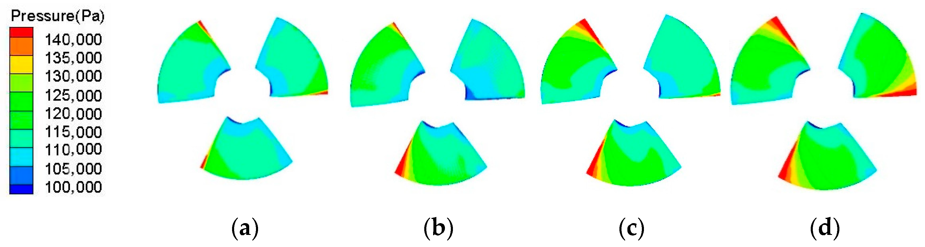
4.2.2. Blade Surface Pressure Analysis

Figure 13 and Figure 14 are the pressure cloud diagrams of the impeller pressure surface and suction surface of different schemes under the design conditions. It can be seen that the pressure distribution trend of each scheme blade is consistent. The comparison between scheme I and scheme IV shows that the increase of the blade placement angle will lead to an increase in the average pressure difference between the front and back of the blade, and the working ability of the impeller will be strengthened. However, due to the increase of the blade angle, the attack angle of the water flow becomes smaller, especially in the back of the scheme IV near the wheel rim, an obvious lower pressure area can be found, indicating that the larger the blade angle is, the easier the backside is to cavitation.

The angles of the three blades of the same impeller in schemes II and III are inconsistent, resulting in an inconsistent trend of blade pressure distribution. The adjacent blades influence each other. The pressure distributions of blade no. 1 in schemes II and III are inconsistent with that of scheme I, and the pressure distributions of blade no. 3 in schemes II and III are inconsistent with that of scheme IV. This condition shows that when the angles of the impeller blades are inconsistent, each blade is no longer in its angle working state. Taking scheme III as an example, because the angle of blade no. 1 of the impeller is small, the pressure difference is small, and the working ability of the blade is weak, while the angle of blade no. 2 and blade no. 3 is large, the pressure difference is large, and the working ability is strong. This condition is reflected in the external characteristic curve of the impeller, where the head of the impeller in schemes II and III is slightly larger than that in scheme I, but lower than that in scheme IV. It can be seen that when the blade angle is deviated, the working ability of the impeller can be improved and the lift of the pump can be increased. The increase in the impeller head is limited, because the adjacent blades influence each other.

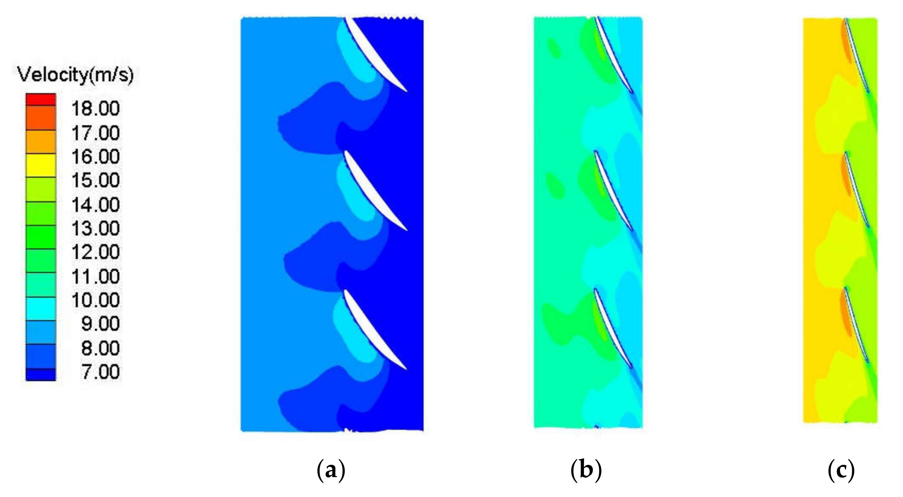
4.2.3. Analysis of Flow Field in Impeller

From the velocity contour of the blade spanning in Figure 15 and Figure 16, it can be seen that the change of the inlet angle of attack due to the placement angle causes the incoming water flow to be biased towards the suction surface of the blade, making the flow velocity at the edge of the suction front higher. In scheme II, the error of blade no.3 becomes larger, which makes the flow field uniformity between adjacent blade channels worse, and the flow velocity distribution is inconsistent. The error angle increases, meaning it is easy to produce cavitation.

At the span = 0.1, the flow state of each span is smooth in scheme I, the periodicity between the blade channels is good, and there are no unstable flow states in the impeller area. However, since the high-speed water flow at the rear of the back of the blade with deviation interferes with the flow state of the inlet of the adjacent blade, the adjacent blades of scheme II are vortex. The inflow condition of the blade no. 3 is changed because its angles are larger. The flow velocity is relatively high on the back of the blades, thereby affecting the flow field of the whole impeller area. The closer to the hub, the stronger the water flow is disturbed by angle deviation. It can be seen from the other two positions that the water flow with different velocities mixes with each other and forms a low-speed area on the back of the 0° blade, which affects the working ability of the blade rim.

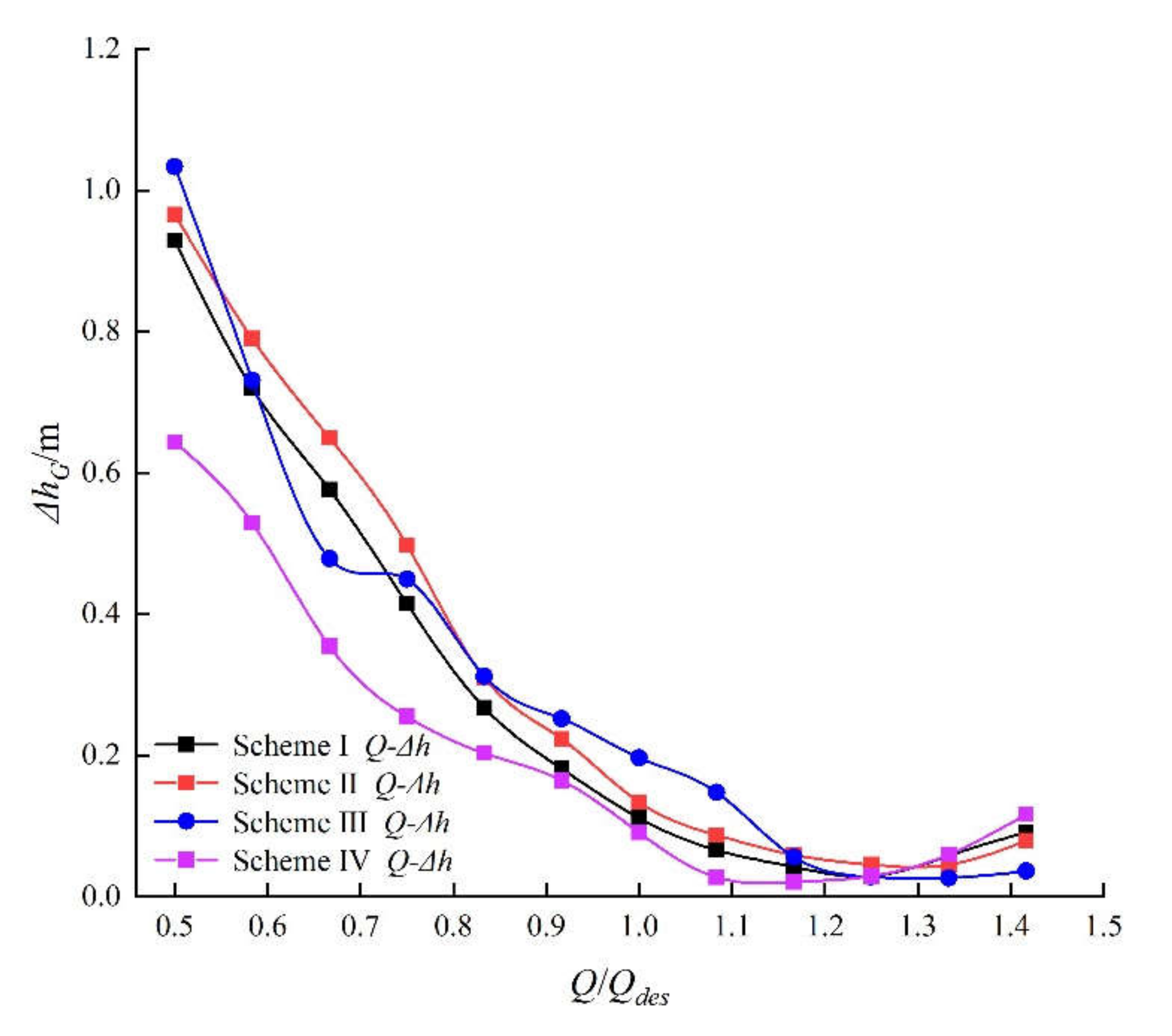
4.2.4. Hydraulic Loss Analysis of Guide Vane and the Outlet Channel

Figure 17 and Figure 18 show the hydraulic loss curves of the guide vane and the outlet channel of the S-type front shaft extension tubular pump device.

In accordance with Figure 17 and Figure 18, the optimal hydraulic loss of the guide vane in different schemes is not much different. The hydraulic loss of the guide vane in scheme I is at least 2.11 cm, and the minimum hydraulic losses of the guide vane in schemes II and III are 2.9 and 4.5 cm, respectively. However, under the small flow conditions, the hydraulic loss of the guide vane in the scheme of the impeller with blade angle deviation is greater than that of the normal scheme. The hydraulic loss of the inlet flow channel is consistent with the change in the discharge coefficient, especially near the best efficiency range and the large flow conditions. This condition shows that the blade angle deviation of the impeller does not affect the flow field of the inlet flow channel. The hydraulic loss of the outlet channel is greatly affected by the blade angle deviation of the impeller. The hydraulic losses of schemes II and III are increased compared with scheme I, especially near the best efficiency range. The blade angle deviation of the impeller has a great influence on the hydraulic loss of the outlet channel of the S-type front shaft extension tubular pump device. Under the design flow conditions, the hydraulic loss of scheme I is 0.13 m, and the hydraulic losses of the outlet channels of schemes II and III are 0.31 and 0.34 m, respectively, which are 2.38 and 2.62 times greater than that of scheme I. The blade angle deviation of the impeller greatly increases the hydraulic loss of the outlet channel.

4.3. Analysis of Structural Characteristic Calculation Results

4.3.1. Blade Deformation Analysis

The impellers of schemes I, II, and III are modeled, and structural characteristic calculations, are performed. The total deformation results of the blades under the different flow conditions of the three schemes are shown in Figure 19 and

Table 3. Maximum total deformation of blades under different working conditions.

Total Deformation(m)	Q/Qdes
	0.7	1	1.2
Scheme I	2.09 × 10−4	1.12 × 10−4	0.34 × 10−4
Scheme II	2.38 × 10−4	1.73 × 10−4	0.91 × 10−4
Scheme III	2.02 × 10−4	1.79 × 10−4	1.20 × 10−4

.

Figure 19 shows the maximum total deformation of different impellers under the design flow condition. The deformation of the blade is proportional, and the maximum deformation is near the rim. The maximum deformation of each scheme is at the rim with the thinnest blade and the furthest distance from the hub near the outlet. In accordance with Table 2, with the increase of flow, the head of the pump decreases, the axial force on the blade decreases, and the total deformation of the blade decreases. When the flow condition Q = 0.7 Q_des, the maximum deformation of scheme I is 0.209 mm, and the max deformation of scheme II is 0.238 mm, which is 1.14 times greater than that of scheme I. When the flow condition Q = 1.0 Q_des, the maximum total deformation of scheme I is 0.112 mm, and the maximum total deformation of scheme III is 0.179 mm, which is 1.60 times greater than that of scheme I. When the flow condition Q = 1.2 Q_des, the maximum total deformation of scheme I is 0.034 mm, and the maximum total deformation of scheme III is 0.12 mm, which is 3.53 times greater than that of scheme I. When the blade angle deviation occurs, the maximum total deformation of the blade increases, and the impeller is more susceptible to damage.

4.3.2. Structural Stress Analysis

The impellers of schemes I, II, and III are modeled, and structural characteristic calculations are performed. The equivalent stress results of the blades under the different flow conditions of the three schemes are shown in Figure 20 and

Table 4. Maximum equivalent stress of pump blades under different working conditions of each scheme.

Equivalent Stress (Pa)	Q/Qdes
	0.7	1	1.2
Scheme I	3.6771 × 107	2.3377 × 107	0.8755 × 107
Scheme II	4.2084 × 107	3.1036 × 107	2.0286 × 107
Scheme III	4.2855 × 107	3.2414 × 107	2.1843 × 107

.

Figure 20 and Table 4 reveal the difference in the equivalent stress distribution of impellers with different schemes. In scheme I, the stress distribution on each blade is consistent, the equivalent stress of the blade shows a decreasing trend, and the maximum equivalent stress occurs in the middle of the hub. When the blade angle increases, the equivalent stress value of the blade increases, which is mainly caused by the increase in water pressure. Under the flow condition Q = 0.7 Q_des, the maximum equivalent stress of scheme I reaches 36.77 MPa, and that of scheme III reaches 42.85 MPa. Under the flow condition Q = Q_des, the maximum equivalent stress of scheme I is 23.37 MPa, and that of scheme III is 32.41 MPa. Under the flow condition Q = 1.2 Q_des, the maximum equivalent stress of scheme I is 8.75 MPa, and the maximum equivalent stress of scheme III is 21.84 MPa, which is 2.5 times greater than that of scheme I.

4.3.3. Structural Modal Analysis

When the axial-flow pump is working normally, the vibration of the impeller causes the liquid around the impeller to vibrate together, and the vibration of the liquid affects the vibration of the impeller. Modal analysis is performed on the impeller to prevent it from being damaged by resonance. Modal analysis is to determine the vibration characteristics of the mechanical structure and calculate its natural frequency and mode shape. The natural frequency is an important parameter in the design of structures subjected to dynamic loads and is the basis for other dynamic analyses.

In this paper, the modal analysis of the impeller is carried out by using the Block Lancos method under prestress, and the various modal orders of the impeller when subjected to gravity, centrifugal force, and water pressure are calculated. The impeller speed n is 1022 r/min, and the impeller frequency is 51.1 Hz. The impeller resonates when the hydraulic excitation frequency is close to its natural frequency. This paper conducts the prestressed modal analysis of the impeller in the air medium under the design conditions and analyzes the natural frequencies of the first six orders of the impeller and the corresponding mode shapes of each order. Figure 21 and Figure 22 show the modes of scheme I and scheme II, respectively.

From the first six-order modal diagram of the impeller in scheme I (Figure 21), the maximum frequency of each scheme gradually increases with the increase in the order, and the vibration forms of the blades are different at each order frequency. From the first-order to third-order modal diagrams where the blade mainly swings up and down (bending vibration), the first-order mode is mainly manifested as three blades swinging back and forth in the same direction at the same time, and the second-order and third-order modes are mainly two blades swinging. The blade deformation from the fourth mode to the sixth mode becomes increasingly complicated. From the sixth mode, the blade is subjected to bending and torsional vibrations, and the vibration form becomes more complex with the increase in frequency. The modes of each order in scheme II (Figure 22) are inconsistent with those of scheme I.

Table 5. Modal natural frequencies.

Schemes	First-Order Mode/Hz	Second-Order Mode/Hz	Third-Order Mode/Hz	Fourth-Order Mode/Hz	Fifth-Order Mode/Hz	Sixth-Order Mode/Hz
Scheme I	699.88	700.48	700.76	1414	1414.5	141.8
Scheme II	699.99	700.64	701.06	1414.7	1415	1416.2
Scheme III	699.97	700.88	701.6	1414.6	1416	1418.9

shows the natural frequencies of the impellers under the design conditions. The first-order vibration frequency of scheme I is 699.88 Hz, which is 13.69 times that of the leaf frequency. The first-order vibration frequency of scheme II is 699.99 Hz, and the vibration frequency changes minimally. Under the same order mode, the difference q1 between the natural frequencies of the impeller blades in each scheme is slightly the same. It can be seen that the angle deviation has little effect on the natural frequency of the pump blade and can be ignored.

5. Conclusions

This paper adopts the research method of numerical simulation combined with model tests to analyze the energy characteristics of the pump device, the hydraulic loss of the flow channel and the structural characteristics of the impeller when the blade angles are inconsistent. This paper analyzes the energy characteristics of the pump device, the impeller work and the internal structural characteristics when the blade placement angles are inconsistent. The main conclusions are as follows:

• The slope of the flow head curve of the pump device is inversely proportional to the placement angle of the guide vane. The highest efficiency point of the S-type tubular pump device is shifted to the large flow condition, and the best efficiency range is gradually widened. The larger the angle of the guide vane, the better it can recover the water flow velocity circulation at the impeller outlet. This condition reduces the hydraulic loss and improves the efficiency of the pump device.
• When blade angle deviation occurs, the flow field of each blade channel is uneven, and the flow field between the blades has mutual influence. The highest efficiency of the S-type front shaft extension tubular pump device of scheme I reaches 76.2%, the highest efficiency of scheme II is 70.4%, the highest efficiency of scheme III is 68.42%, and the maximum efficiency drop reaches 7.78%. The blade angle deviation has minimal effect on the efficiency of the impeller and the hydraulic loss of the guide vane, and the main reason for the decrease in efficiency is the increase in hydraulic losses in the outlet flow channel.
• The maximum deformation of scheme I is 0.034 mm, and the max deformation of scheme III is 0.12 mm, which is 3.53 times greater than that of scheme I. The maximum equivalent stress of scheme I is 8.75 MPa, and the maximum equivalent stress of scheme III is 21.84 MPa, which is 2.50 times greater than that of scheme I. The deviation of the blade angle often leads to an increase in the maximum equivalent stress and maximum deformation of the impeller, which is more obvious under large flow conditions. The natural modal vibration frequency of the impeller with prestress is slightly the same with or without the blade angle deviation.

References

1. Liu, C. Researches and Developments of Axial-flow Pump System. Trans. Chin. Soc. Agric. Mach. 2015, 46, 49–59. [Google Scholar]
2. Liu, C. Pumps and Pumping Stations; China Water Resources and Hydropower Press: Yangzhou, China, 2009. [Google Scholar]
3. Qian, Z.; Wang, F.; Guo, Z.; Lu, J. Performance evaluation of an axial-flow pump with adjustable guide vanes in turbine mode. Renew. Energy 2016, 99, 1146–1152. [Google Scholar] [CrossRef]
4. Shi, L.; Yuan, Y.; Jiao, H.; Tang, F.; Cheng, L.; Yang, F.; Jin, Y.; Zhu, J. Numerical investigation and experiment on pressure pulsation characteristics in a full tubular pump. Renew. Energy 2021, 163, 987–1000. [Google Scholar] [CrossRef]
5. Feng, X.; Qiu, B. Adjusting Frequency of Pump Blade Angles and Optimal Operation for Large Pumping Station System. Adv. Mech. Eng. 2013, 5, 317517. [Google Scholar] [CrossRef]
6. Yao, Y.; Chao, L. Study on similarity of pump blade adjusting performances. J. Hydroelectr. Eng. 2013, 32, 76–281. [Google Scholar]
7. Yao, Y. Study on Optimal Operation of Pumping Stations based on Ant Colony Optimization Algorithm and Similarity of Pump Blade Adjusting. Ph. D. Thesis, Yangzhou University, Yangzhou, China, 2013. [Google Scholar]
8. Zhang, W.; Tang, F.; Xie, R. Analysis of the Variable Angle and Speed of the Axial Flow Pumps. China Rural. Water Hydropower 2016, 186–188. [Google Scholar]
9. Shi, L.; Fu, L.; Liu, C.; Tang, F.; Zhang, W.; Chen, F. Impacts of the Angle of Attack on Hydraulic Characteristics over the Axial flow Impeller. J. Irrig. Drain. 2019, 38, 55–62. [Google Scholar]
10. Wu, Z.; Hou, C.; Liang, W.; He, D. Effect of blade installation angle on cavitation performance of axial flow pump. Chin. J. Hydrodyn. 2020, 35, 277–284. [Google Scholar]
11. Wu, X.; Lu, Y.; Tan, M.; Liu, H. Effect of vane angle on axial flow pump running characteristics in saddle zone. Trans. Chin. Soc. Agric. Eng. 2018, 34, 46–53. [Google Scholar]
12. Velarde, S.; Tajadura, R. Numerical simulation of the aerodynamic tonal noise generation in a backward-curved blades centrifugal fan. J. Sound Vib. 2006, 295, 781–786. [Google Scholar]
13. Cravero, C.; Marsano, D. Numerical prediction of tonal noise in centrifugal blowers. In Proceedings of the Turbo Expo 2018: Turbomachinery Technical Conference & Exposition, Oslo, Norway, 11–15 June 2018. ASME Paper GT2018-75243. [Google Scholar]
14. Ding, H.; Chang, T.; Lin, F. The Influence of the Blade Outlet Angle on the Flow Field and Pressure Pulsation in a Centrifugal Fan. Processes 2020, 8, 1422. [Google Scholar] [CrossRef]
15. Bing, H. Effects of blade rotation angle deviations on mixed-flow pump hydraulic performance. Sci. China Technol. Sci. 2014, 57, 1372–1382. [Google Scholar] [CrossRef]
16. Bing, H.; Cao, S.; He, C.; Lu, L. Experimental study of the effect of blade tip clearance and blade angle error on the performance of mixed-flow pump. Sci. China Technol. Sci. 2013, 56, 293–298. [Google Scholar] [CrossRef]
17. Yulong, L. Effects of blade deflector structure on the cavitation and fluid-solid coupling characteristics of an axial flow pump. Ph. D. Thesis, Xi’an University of Technology, Xi’an, China, 2021. [Google Scholar]
18. Dorji, U.; Ghomashchi, R. Hydro turbine failure mechanisms: An overview. Eng. Fail. Anal. 2014, 44, 136–147. [Google Scholar] [CrossRef]
19. Guangkuan, W.; Xingqi, L.; Jianjun, F. Cracking reason for Francis turbine blades based on transient fluid structure interaction. Trans. Chin. Soc. Agric. Eng. 2015, 31, 92–98. [Google Scholar]
20. Shi, L.; Zhu, J.; Wang, L.; Chu, S.; Tang, F.; Jin, Y. Comparative Analysis of Strength and Modal Characteristics of a Full Tubular Pump and an Axial Flow Pump Impellers Based on Fluid-Structure Interaction. Energies 2021, 14, 6395. [Google Scholar] [CrossRef]
21. Shi, L.; Zhu, J.; Tang, F.; Wang, C. Multi-Disciplinary Optimization Design of Axial-Flow Pump Impellers Based on the Approximation Model. Energies 2020, 13, 779. [Google Scholar] [CrossRef] [Green Version]
22. Shi, L.; Zhu, J.; Yuan, Y.; Tang, F.; Huang, P.; Zhang, W.; Liu, H.; Zhang, X. Numerical Simulation and Experiment of the Effects of Blade Angle Deviation on the Hydraulic Characteristics and Pressure Pulsation of an Axial-Flow Pump. Shock. Vib. 2021, 2021, 1–14. [Google Scholar] [CrossRef]
23. Zhang, Z.; Zheng, Y.; Zhang, X. Modal Analysis Based on Fluid-Structure Interaction of Axial Flow Rotor. Appl. Mech. Mater. 2015, 799–800, 565–569. [Google Scholar] [CrossRef]
24. Kan, K.; Zheng, Y.; Chen, H.; Cheng, J.; Gao, J.; Yang, C. Study into the Improvement of Dynamic Stress Characteristics and Prototype Test of an Impeller Blade of an Axial-Flow Pump Based on Bidirectional Fluid–Structure Interaction. Appl. Sci. 2019, 9, 3601. [Google Scholar] [CrossRef] [Green Version]
25. Kan, K.; Zheng, Y.; Fu, S.; Liu, H.; Yang, C.; Zhang, X. Dynamic stress of impeller blade of shaft extension tubular pump device based on bidirectional fluid-structure interaction. J. Mech. Sci. Technol. 2017, 31, 1561–1568. [Google Scholar] [CrossRef]
Figure 1. Model diagram of S-type front shaft extension tubular pump device. (1). Inlet channel. (2). S-elbow pipe. (3). Impeller. (4). Guide vane body. (5). Outlet channel.
Processes 10 00328 g001
Figure 2. The impeller of an axial flow pump.
Processes 10 00328 g002
Figure 3. Grid independence analysis.
Processes 10 00328 g003
Figure 4. Grid division of the Fluid Domain. (a) The grids of S-type front shaft extension tubular pump device. (b) The grid of the impeller.
Processes 10 00328 g004
Figure 5. The finite element mesh of the impeller.
Processes 10 00328 g005
Figure 6. Model pump device. (a) Impeller. (b) Guide vane. (c) Pump device installation. (1). Inlet channel. (2). S-typed elbow pipe. (3). Impeller chamber. (4). Guide vane. (5). Outlet channel.
Processes 10 00328 g006
Figure 7. Performance comparison between numerical simulation and model test.
Processes 10 00328 g007
Figure 8. Guide vane models with different design parameters. (a) Front view of guide vane. (b) Top view of guide vane.
Processes 10 00328 g008
Figure 9. Calculation results of the hydraulic performance of S-type front shaft extension tubular pump device (different guide vane schemes).
Processes 10 00328 g009
Figure 10. Hydraulic loss of guide vane (different guide vane schemes).
Processes 10 00328 g010
Figure 11. Performance curve of pump device in different schemes.
Processes 10 00328 g011
Figure 12. Hydraulic performance curve of axial-flow pump impeller in different schemes.
Processes 10 00328 g012
Figure 13. Pump blade frontal pressure distribution of different schemes (Q = Qdes). (a) Scheme I. (b) Scheme II. (c) Scheme III. (d) Scheme IV.
Processes 10 00328 g013
Figure 14. Pressure distribution on the back of the blade of different schemes (Q = Qdes). (a) Scheme I. (b) Scheme II. (c) Scheme III. (d) Scheme IV.
Processes 10 00328 g014
Figure 15. Velocity contour of each span in scheme I (Q = Qdes). (a) Span = 0.1. (b) Span = 0.5. (c) Span = 0.9.
Processes 10 00328 g015
Figure 16. Velocity contour of each span in scheme II (Q = Qdes). (a) Span = 0.1. (b) Span = 0.5. (c) Span = 0.9.
Processes 10 00328 g016
Figure 17. Hydraulic loss curves of guide vanes in different schemes.
Processes 10 00328 g017
Figure 18. Hydraulic loss curves of outlet channel in different schemes.
Processes 10 00328 g018
Figure 19. Impeller total deformation distribution under Qdes in different schemes. (a) Scheme I. (b) Scheme II. (c) Scheme III.
Processes 10 00328 g019
Figure 20. Equivalent stress distribution under Qdes in different schemes. (a) Scheme I. (b) Scheme II. (c) Scheme III.
Processes 10 00328 g020
Figure 21. The mode shape changes of scheme I in each mode. (a) First-order mode. (b) Second-order mode. (c) Third-order mode. (d) Fourth-order mode. (e) Fifth-order mode. (f) Sixth-order mode.
Processes 10 00328 g021
Figure 22. The mode shape changes of scheme II in each order mode. (a) First-order mode. (b) Second-order mode. (c) Third-order mode. (d) Fourth-order mode. (e) Fifth-order mode. (f) Sixth-order mode.
Processes 10 00328 g022