Article

Numerical Simulation of Hydraulic Fracturing and Penetration Law in Continental Shale Reservoirs

1
School of Petroleum Engineering, Yangtze University, Wuhan 430100, China
2
Key Laboratory of Drilling and Production Engineering for Oil and Gas, Wuhan 430100, China
3
Gudao Oil Production Plant of Shengli Oilfield Co., Ltd., Dongying 257231, China
4
Petroleum Engineering Technology Research Institute of Jianghan Oilfield, Sinopec, Wuhan 430000, China
*
Authors to whom correspondence should be addressed.
Processes 2022, 10(11), 2364; https://doi.org/10.3390/pr10112364
Submission received: 6 October 2022 / Revised: 28 October 2022 / Accepted: 1 November 2022 / Published: 11 November 2022

Abstract

:
The vertical heterogeneity of continental shale reservoirs is strong, the difference between lithology and stress between layers is large, the weak interface between layers develops, and the hydraulic fracture penetration and expansion are difficult, resulting in poor fracturing transformation effect. In view of this, based on the finite element and cohesive element method, this paper established a fluid-solid coupling model for the hydraulic fracture propagation through the continental shale and studied the control mechanism and influence law of various geological and engineering parameters on the hydraulic fracture propagation through the continental shale reservoir using single factor and orthogonal test analysis methods. Interfacial cementation strength between high layers, high vertical stress difference, low interlaminar stress difference, low tensile strength difference, low elastic modulus difference, high pressure fracturing fluid viscosity, and high injection displacement are conducive to the penetration and expansion of hydraulic fractures. The primary and secondary order of influence degree of each factor is: interlaminar interface cementation strength > interlaminar stress difference/tensile strength difference > fracturing fluid viscosity/injection displacement > vertical stress difference > elastic modulus. In addition, engineering application research has also been carried out, and it is recommended that the injection displacement during early construction should not be less than 3 m3/min, and the fracturing viscosity should not be less than 45 mPa·s. The field application effect is good, which verifies the engineering application value of the model.

1. Preface

The exploration and development of shale gas have a long history of nearly 200 years. Shale gas in North America has developed rapidly, realizing efficient, economic and large-scale development, becoming an important source of natural gas supply in North America, and causing significant changes in the global natural gas supply pattern [1,2,3]. Countries in Europe, Oceania, South America and other regions have fully recognized the value and prospects of shale gas resources and have started extensive shale gas research, exploration and development, such as basic theoretical research, resource potential evaluation, and industrial production tests [4,5,6]. China is rich in shale gas resources, with recoverable reserves of about 25.08 × 10¹² m3 and huge development potential [7]. After more than 10 years of development, the theory and key technologies for the effective large-scale development of shallow marine shale gas above 3500 m have been basically mastered, but few breakthroughs have been made in the development of continental shale gas [8]. Compared with marine shale, continental shale reservoirs have strong vertical heterogeneity, large differences in interlayer lithology and stress, developed weak interfaces between layers, and it is difficult for hydraulic fractures to propagate through layers, resulting in ineffective fracturing stimulation [9]. Therefore, it is urgent to carry out research on the propagation law of hydraulic fractures in continental shale.
At present, many scholars at home and abroad have carried out a series of studies from laboratory experiments [10,11,12,13,14,15,16,17,18,19,20] and numerical simulations [21,22,23,24,25,26,27,28] on the propagation law of hydraulic fractures in stratified reservoirs. Some scholars have carried out a large number of laboratory experiments on multi-lithologic combination layered rock samples such as concrete, sandstone and coal rock using a true triaxial large-scale fracturing physical simulation device and studied the influence of various geological and engineering parameters on the propagation of hydraulic fractures through layers. The experimental results show that the hydraulic fractures in the layered rock samples exhibit asymmetric and non-planar expansion characteristics in the vertical direction. After encountering the interface between layers, it presents a variety of complex expansion modes such as stopping, turning, forking and penetrating dot difference in the elastic modulus of the reservoir/barrier rock does not have a significant inhibitory effect on the propagation of hydraulic fractures through the interlayer, the horizontal minimum stress difference between layers, the vertical stress difference (the difference between the vertical stress and the horizontal minimum stress), the properties of the interlayer interface, the injection displacement and the viscosity of the fracturing fluid are the key factors that determine whether a hydraulic fracture can penetrate the layer; the smaller the minimum horizontal stress difference between layers, the greater the vertical stress difference, the higher the interface cementation strength, the higher the injection displacement and the higher the viscosity of the fracturing fluid, the more favorable the hydraulic fractures to achieve through-layer expansion [14,15,16,17,18,19,20]. Laboratory experiments have initially revealed the propagation law of hydraulic fractures through layers, but they can only provide some qualitative understanding and have limited guiding significance for the optimal design of hydraulic fracturing. Therefore, some scholars based on the displacement discontinuity method (DDM) [21,22], finite element (FEM) and cohesive element (cohesive element) method [23,24,25], extended finite element method (XFEM) [26], and numerical methods such as discrete element method (DEM) [27,28] have established a series of numerical models of hydraulic fracture penetration through layers, and carried out a large number of studies on influencing factors, further revealing the law of hydraulic fracture penetration through layers, which is a quantitative prediction method. The propagation pattern of hydraulic fracture through the layer provides an effective means.
The above studies show that various geological and engineering parameters have a significant impact on the propagation law of hydraulic fractures through layers, but the primary and secondary relationship between these factors has not been elucidated, and most of these studies are carried out on sandstone or coal rock reservoirs, which cannot systematically reveal the propagation law of hydraulic fractures in continental shale reservoirs. Therefore, in view of the development characteristics of continental shale reservoirs, this paper establishes a fluid-solid coupling model of continental shale hydraulic fractures spreading through layers based on the finite element and cohesive element method, and the model is verified by analytical solutions and experimental laboratory results. Carry out a single-factor analysis and orthogonal test research to systematically reveal the propagation law of hydraulic fractures in continental shale reservoirs.

2. Mathematical Model

In layered reservoirs, the hydraulic fracture height is usually much smaller than its length, and the fluid pressure in the fracture changes little along the fracture length except for the fracture tip. The strain model can give reasonable results [29]. Based on this, a two-dimensional plane strain model of continental shale hydraulic fractures spreading through layers is established in this paper.

2.1. Fluid-Structure Interaction Governing Equation

In the process of hydraulic fracturing, the deformation of the rock skeleton interacts with and influences the fluid flow in the pore space. The effective stress principle can be used to characterize the stress-seepage coupling relationship in the rock. Take the control volume V and its surface as S, then the rock. The coupled governing equation of solid skeleton deformation and fluid flow is [29]:
V σ ¯ p w Ι · δ ε d V = S t · δ v d S + V f · δ v d V
In the formula, σ ¯ is the effective stress matrix, Pa; pw is the pore pressure, Pa; I is the unit matrix, dimensionless; δε is the virtual strain rate matrix, s−1; δv is the virtual velocity vector, m/s; t is the surface force vector, N/m2; f is the body force vector, N/m3.
The mass conservation equation of fluid seepage in the pores of the rock skeleton is:
V 1 J d d t J ρ w φ w d V + S ρ w φ w n T · v w d S = 0
Among them, the flow velocity, vw, of the fluid in the rock satisfies Darcy’s law [17,19,24,29]:
v w = 1 φ w g ρ w k p w x ρ w g
In the formula, J is the rock volume change rate, dimensionless; ρw fluid density, kg/m3; φw is the porosity, dimensionless; nT is the outer normal direction vector of the surface S, dimensionless; x is the space vector, m; g is the gravitational acceleration vector, m/s2; k is the rock skeleton permeability tensor, m/s.

2.2. Criteria for Crack Initiation and Propagation

In this paper, the cohesive element is used to simulate the initiation and propagation of hydraulic fractures and weak bedding planes, and the secondary nominal stress criterion is used to determine whether the cracks initiate or not:
σ n σ n o 2 + τ s τ s o 2 = 1
where
σ n = σ n σ n 0 0 σ n < 0
where σn and τs are the normal and tangential stresses actually borne by the cohesive element, Pa; σno and τso are the tensile strength and shear strength of the rock, Pa.
The crack propagation process is described by the stiffness degradation criterion of the cohesive element, and its expression is as follows:
σ n = 1 D σ n ¯ σ n ¯     0 σ n ¯ σ n ¯   <   0 τ s = 1 D τ s ¯
In the formula, σ n ¯ and τ s ¯ are the stress calculated by the normal and tangential direction of the cohesive element under the current strain according to the undamaged front-line elasticity criterion, respectively; D is the damage factor, dimensionless, ranging from 0 to 1, when D = 0, the material is not damaged. When D = 1, the material is completely damaged; that is, the hydraulic crack begins to expand (as shown in Figure 1). The calculation formula is as follows:
D = δ f δ m δ o δ m δ f δ o
In the formula, δo and δf are the displacement at the initial damage and the displacement when the element is completely damaged, m; δm is the maximum displacement reached during the loading process, m.

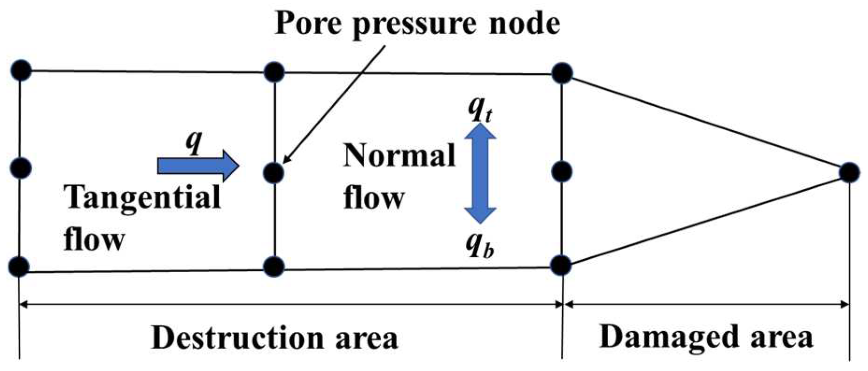
2.3. Fluid Flow Equation in Fractures
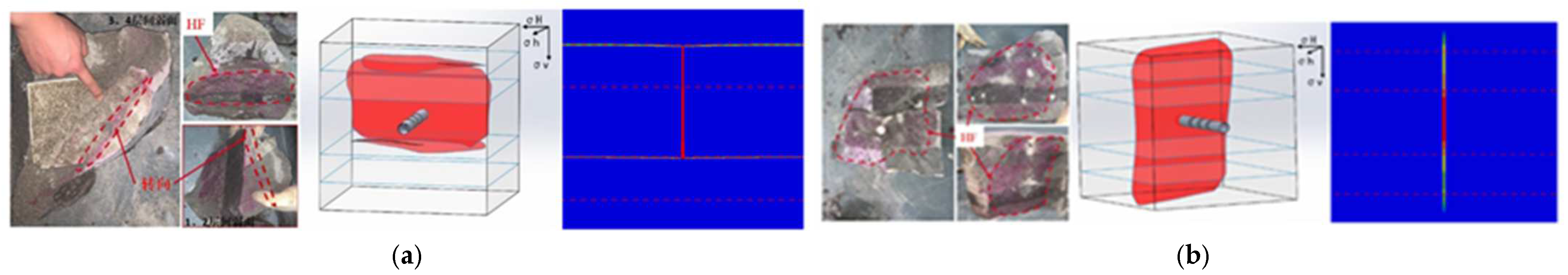
After the cohesive cell is completely damaged, fluid will enter the damaged cell. As shown in Figure 2, there are two flow states of fluid in the damaged unit, which are divided into tangential flow and normal flow.
In this paper, the fracturing fluid is assumed to be an incompressible Newtonian fluid, and the formula for its tangential flow is:
q = w 3 12 μ p
The formula for calculating normal flow is:
q t = c t p f p t q b = c b p f p b
where q is the tangential flow rate, m3/s; μ is the fracturing fluid viscosity, Pa·s; w is the fracture width, m; ∇p is the tangential pressure gradient of the cohesive unit, Pa/m; qt, qb is the normal flow into the upper and lower surfaces of the unit, m3/s; ct, and cb are the filtration coefficients of the upper and lower surfaces, m3/(Pa·s), pt and pb are the pore pressures at the upper and lower surfaces of the fracture, Pa; pf is the fluid pressure in the fracture, Pa.

3. Model Validation

ABAQUS finite element analysis software was used to build and solve the above model, and the model solution accuracy was closely related to the mesh size. In order to determine a reasonable mesh size, the classical KGD hydraulic fracture propagation model was constructed using ABAQUS software, the mesh size was set to 1 m × 1 m, 0.2 m × 0.2 m and 0.1 m × 0.1 m, the calculation parameters are shown in Table 1, and the solution results were compared with the analytical solution. The calculation formula of the analytical solution is [30]:
L t = 1 4 π 1 3 E q t 1 v 2 K I C 2 3 W t = 32 π 2 1 3 K I C 2 q t 1 v 2 2 E 2 1 3
where E is elastic modulus, MPa; v is Poisson’s ratio, dimensionless; KIC is rock fracture toughness, MPa∙m0.5; q is displacement per unit fracture height, m2/s; L(t) is the half-foil length of the hydraulic fracture at time t, m; W(t) is the width of the hydraulic fracture at the injection point at time t, m; t is the injection time of the fracturing fluid, s. As shown in Figure 3, When the grid size is 1 m, the difference between the simulation results and the analytical solution is large, and the curve has large fluctuations. When the grid size is 0.2 and 0.1, and the half length of the hydraulic fracture exceeds 5 m, that is, 25× the side length of the grid element, the numerical simulation results agree well with the analytical solution. Based on this, the construction and meshing of the subsequent numerical model adopt the above-mentioned mesh size setting standard; that is, the edge length of the mesh element is less than 50× the size of the simulated fracture.
In order to further verify that the numerical simulation method has the ability to simulate the propagation behavior of continental shale hydraulic fractures through layers, the laboratory experiment results were used to verify it [20]. Referring to the above meshing standards, the simulation is carried out using the parameters in Table 2. As shown in Figure 4, under the conditions of different fracturing fluid viscosity, the hydraulic fracture morphology obtained by numerical simulation is basically consistent with the experimental laboratory results, which verifies the accuracy of this numerical simulation method.

4. Analysis of Influencing Factors of Hydraulic Fractures through Layer Propagation

4.1. Model Establishment and Parameters

As shown in Figure 5a, assuming that the hydraulic fracture shape is symmetrical about the injection point, in order to improve the calculation efficiency, a 40 m × 40 m semi-model of continental shale hydraulic fracture penetration through layers is established. The upper part of the model is an interlayer, the lower part is the thickness of the reservoir is 20 m, and the grid unit size is 0.2 m × 0.2 m. The basic input parameters are shown in Table 3. Based on this model, the single-factor analysis method was used to study the influence of various geological and engineering parameters on the propagation of hydraulic fractures through layers. The simulation results are shown in Figure 5b–f.

4.2. Influence of Formation Parameters

4.2.1. Bonding Strength of Interlayer Interface

The interfacial cementation strength of continental shale is closely related to the cement type (quartz, calcite or pyrite, etc.) and content and is usually quantitatively characterized by the interface shear strength [9,24]. The higher the cementation strength, the higher the interface shear strength. The shear strengths of the interlayer interface in the four groups of simulation examples in Figure 5b are 1.2 MPa, 2.4 Mpa, 3.6 Mpa and 4.8 Mpa, respectively. All show the simulation results under the same injection volume (the same as below). The simulation results show that the bonding strength of the interlayer interface has an important influence on the vertical propagation path of hydraulic fractures. When the bonding strength of the interlayer interface is low, the hydraulic fracture activates the interlayer interface and extends along it, and the vertical expansion is hindered; on the contrary, the hydraulic fracture penetrates the interlayer interface, enters the interlayer and continues to expand, and the interlayer interface is cemented at this time. The strengths (3.6 MP and 4.8 Mpa) have basically no effect on the vertical propagation shape of hydraulic fractures. The reason is that during the fracturing process, the interface between weakly cemented layers is more prone to shear slip under the combined action of the induced stress at the tip of the hydraulic fracture and the filtration of the fracturing fluid along the interface, resulting in the rapid release of fracturing energy and the failure of the hydraulic fracture penetrating the interlayer interface [21].

4.2.2. Vertical Stress Difference

The vertical stress difference is defined as the difference between the vertical in-situ stress and the minimum horizontal in-situ stress. The vertical in-situ stresses of the four groups of calculation examples in Figure 5c are 37 Mpa, 39 Mpa, 41 Mpa and 43 Mpa, respectively; that is, the vertical stress differences are 2 Mpa, 4 Mpa, 6 Mpa and 8 Mpa, respectively. The simulation results show that with the increase of the vertical stress difference, the ability of hydraulic fractures to penetrate through layers is significantly enhanced, and the height of hydraulic fractures increases. According to the classic Renshaw & Pollard criterion [31], when the minimum horizontal in-situ stress remains unchanged, the greater the vertical stress difference, the stronger the ability of the interlayer interface to resist shear failure, thereby avoiding shear slip caused by the interlayer interface. The vertical expansion of hydraulic fractures is hindered. In the above case, the critical vertical stress difference for hydraulic fractures to penetrate the interlayer interface is about 4 Mpa.

4.2.3. Interlayer Stress Difference

The interlayer stress difference is defined as the difference between the minimum horizontal in-situ stress of the interlayer and the reservoir. In Figure 5d, the minimum horizontal in-situ stresses of the interlayers of the four groups of calculation examples are 33 Mpa, 35 Mpa, 37 Mpa and 39 Mpa, respectively; that is, the interlayer stress differences are −2 Mpa, 0 Mpa, 2 Mpa and 4 Mpa, respectively. The simulation results show that the smaller the interlayer stress difference, the stronger the ability of hydraulic fractures to penetrate through the layers and the greater the fracture height. According to the classic Renshaw & Pollard criterion [31], the greater the interlayer stress difference, the more difficult it is for hydraulic fractures to penetrate the interlayer interface. Even if the interlayer interface penetrates, the minimum horizontal in-situ stress of the high interlayer means high extension resistance, and the height of the hydraulic fractures will also be significantly suppressed, forming “short and wide” fractures.

4.2.4. Poor Tensile Strength

The tensile strength difference is defined as the difference in the tensile strength of the barrier and the reservoir. In Figure 5e, the interlayer tensile strength of each calculation example is 2 Mpa, 4 Mpa, 6 Mpa and 8 Mpa, respectively; that is, the interlayer tensile strength difference is −2 Mpa, 0 Mpa, 2 Mpa and 4 Mpa, respectively. The simulation results show that the effect of the difference in tensile strength on the propagation of hydraulic fractures through layers is basically consistent with the difference in interlayer stress. Because in addition to the minimum horizontal in-situ stress, the tensile strength of the rock needs to be overcome in the process of hydraulic fracture extension; that is, when hydraulic fractures start from high-strength layers, it is easier to penetrate the interlayer interface into low-strength layers and propagate, which is consistent with the published numerical simulation [18] and laboratory experiments [24] results. Based on this, the wellbore traversing horizon and perforation horizon of the fracturing well can be optimized.

4.2.5. Elastic Modulus Difference

The elastic modulus difference is defined as the difference between the elastic moduli of the barrier and the reservoir. The elastic moduli of the interlayers of the four groups of calculation examples in Figure 5f are 10 Gpa, 20 Gpa, 30 Gpa, and 40 Gpa, respectively; that is, the interlayer elastic moduli differences are −10 Gpa, 0 Gpa, 10 Gpa, and 20 Gpa, respectively. The simulation results show that the influence of the elastic modulus difference on the vertical propagation path of hydraulic fractures is not significant, and this understanding has been verified by the laboratory and mine experimental results [32]; In the case of good interlayer interface bonding strength, high elastic modulus difference is a favorable factor for hydraulic fractures to achieve through-layer expansion, because when the hydraulic fracture enters the high elastic modulus interlayer, its width will be suppressed, and it is more likely to form “high and narrow” fractures. However, if the elastic modulus of the interlayer is too high, the width of the hydraulic fracture is too narrow, and the proppant migration is hindered. Even if the dynamic fracture extends to this point, it is difficult to obtain effective support after the fracture is closed, and the improvement of the fracturing effect is limited. Overall, the effect of elastic modulus on the propagation behavior of hydraulic fractures is not as significant as that of other geological factors.

4.3. Influence of Construction Parameters

4.3.1. Fracturing Fluid Viscosity

The fracturing fluid viscosities of the four groups of examples in Figure 6a are 10 mPa·s, 30 mPa·s, 50 mPa·s, and 70 mPa·s, respectively. The simulation results show that high-viscosity fracturing fluid is a favorable factor for hydraulic fractures to achieve through-layer propagation. The higher the viscosity of the fracturing fluid, the smaller the filtration loss, the greater the net pressure in the fracture, and the more sufficient the hydraulic energy, which is conducive to the continuous expansion of hydraulic fractures through the interlayer interface [33]. On the contrary, the lower the viscosity of fracturing fluid is, the lower the net pressure in the fracture is, and the weaker the hydraulic energy is. In addition, low-viscosity fracturing fluid is more likely to invade the bedding interface to produce lubrication and pressure holding, which will induce the shear slip of the interlayer interface, resulting in the rapid release of hydraulic energy, which will lead to the hydraulic fracture being captured by the interlayer interface and the vertical expansion being blocked. In addition, when the viscosity of the fracturing fluid exceeds a certain critical value (30 mPa·s), with further increases in the viscosity, the width of the fracture increases and the height decreases, forming a “short and wide” fracture. Therefore, although the high-viscosity fracturing fluid is beneficial to achieve interlayer expansion, excessively increasing the viscosity of the fracturing fluid can certainly achieve the ideal fracture height.

4.3.2. Injection Displacement

The injection displacements of the four groups of calculation examples in Figure 6b are 0.6 m3/min, 1.8 m3/min, 3 m3/min and 4.2 m3/min, respectively. The simulation results show that the influence of the injection displacement on the propagation behavior of hydraulic fractures is similar to that of the fracturing fluid viscosity because increasing the injection displacement is also beneficial to increase the net pressure in the fractures and enhance the ability of hydraulic fractures to penetrate the interface between layers. Theoretical studies show that, in the case of ignoring fracturing fluid filtration, the net pressure in the fracture is a function of the product of the injected displacement and the fracturing fluid viscosity when the fluid injection volume is the same, that is, increasing the injection displacement or fracturing fluid viscosity by the same multiple should have the same enhancement effect on the ability of hydraulic fractures to penetrate through layers [34]. However, the simulation results in Figure 6 do not support the above conclusion. Increasing the injection displacement does not improve the penetration effect of hydraulic fractures as much as increasing the viscosity of the fracturing fluid. The main reason is that the above calculation example does not ignore the filtration behavior of fracturing fluid, which is more in line with the real situation. And in the actual fracturing construction process, due to the limitation of construction equipment, the injection displacement cannot be increased by tens or even hundreds of multiples like the viscosity of the fracturing fluid. Therefore, it is recommended to increase the viscosity of the fracturing fluid to enhance the ability of hydraulic fractures to penetrate through layers during on-site construction.

4.4. Primary and Secondary Relationship of Key Influencing Factors

To sum up, the mechanism of the hindered propagation of hydraulic fractures through layers is: (1) The shear slip at the interlayer interface changes the vertical expansion path of hydraulic fractures, limiting the growth of fracture height; (2) The width of hydraulic fractur.es is large, which weakens the growth of fracture height’s ability. The former has a more significant effect and is mainly controlled by factors such as interlayer interface strength, vertical stress difference, interlayer stress difference, tensile strength difference, and fracturing fluid viscosity. In order to further reveal the primary and secondary relationship of these influencing factors, an orthogonal numerical simulation experiment was carried out based on the above numerical model [35]. Since the effect of tensile strength difference on the propagation of hydraulic fractures through interlayer is basically the same as that of interlayer stress difference, in order to reduce the number of orthogonal experiment groups, this paper introduces the extension resistance difference to characterize the composite effect of these two factors on the propagation of hydraulic fractures through the layer, which is defined as the sum of the difference in tensile strength and the difference in interlayer stress. Based on this, an orthogonal experiment with four factors and three levels was designed. The specific scheme and results are shown in Table 4 and Table 5.
It can be seen from Table 5 that IIIIA > IIIA> IIA, IIIIB > IIIB > IIB, IIC > IIIC > IIIIC, IIIID > IIID > IID, indicating that the greater the vertical stress difference, the greater the shear strength of the interlayer interface, the smaller the extension resistance difference, and the greater the viscosity of the fracturing fluid, the better the hydraulic fracture propagation effect through the layer, which is consistent with the previous law; TB >TC >TD >TA, indicating that the priority order of the four key influencing factors is: interlayer interface shear strength > extension resistance difference (interlayer stress difference/tensile strength difference) > fracturing fluid viscosity > vertical stress difference.

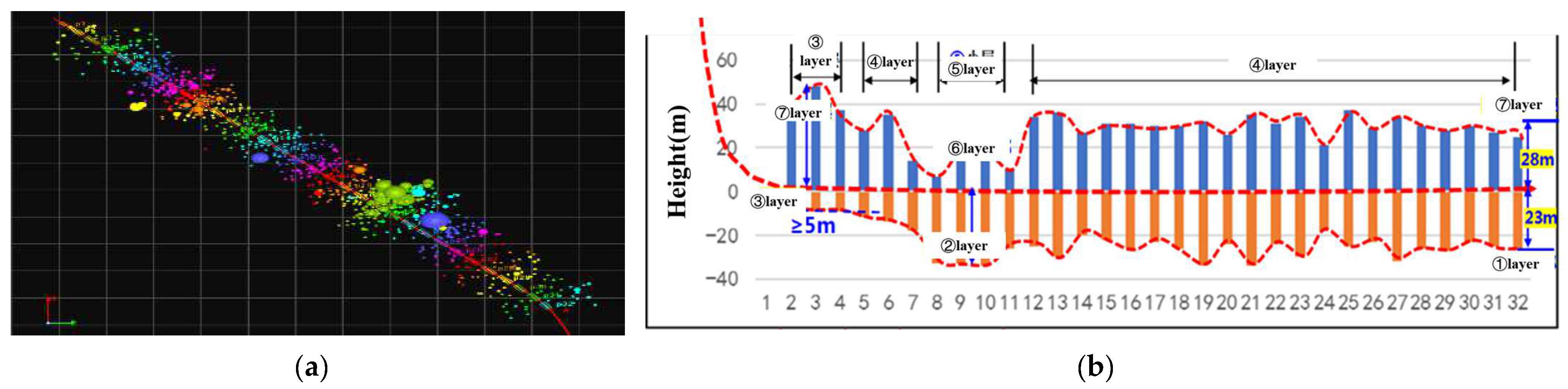
5. Engineering Applications

Taking the FYH10 continental shale gas horizontal well as an example, the target interval of the well is divided into seven sublayers, and the horizontal wellbore mainly passes through the ④ sublayer, of which the ①–④ sublayers are high-quality shale gas reservoirs and are the key layers for fracturing stimulation, the rock’s mechanical properties and in-situ stress of each sublayer are quite different (see Table 6), which makes the vertical expansion of hydraulic fractures difficult. Based on this, referring to the basic parameters in Table 6, the finite element and cohesive element method is used to establish a hydraulic fracture penetration expansion model, and carry out a case study to optimize the construction displacement and viscosity parameters, so as to obtain a better penetration fracturing effect. The simulation results are shown in Figure 7.
It can be seen from Figure 7 that with the increase of displacement and viscosity, the ability of hydraulic fractures to penetrate layers is significantly enhanced when the displacement is not less than 3 m3/min and the viscosity is not less than 45 mPa·s, and hydraulic fractures can achieve the effect of communicating ①–④ small layers. Based on the above optimization results, the well is divided into 32 stages for fracturing, with five to six clusters of perforations per stage, and the injection displacement is 15–18 m3/min, 50 mPa·s high-viscosity fracturing fluid was used to realize hydraulic fracture penetration and expansion during construction, and then 5 mPa·s low-viscosity slick water was used to improve the complexity of hydraulic fractures. As shown in Figure 8, the microseismic monitoring results show that the hydraulic fractures in each fracturing section have ideal height expansion and basically achieve the effect of penetrating the small layers ①–④, and a large-scale complex fracture network is formed in the reservoir, the daily gas production was 5.58 × 10⁴ m3, and the daily oil production was 17.6 m3 after the pressure test, and a good production increase effect was achieved.

6. Conclusions

(1)
Based on the finite element and cohesive element method, a fluid-solid coupling model of continental shale hydraulic fractures spreading through layers was established, and the accuracy of the model was verified by comparing it with analytical solutions and experimental laboratory results. Based on this model, single-factor and orthogonal test analysis methods are used to reveal the control mechanism and law of various geological and engineering parameters on the propagation behavior of hydraulic fractures;
(2)
The hindered mechanism of hydraulic fracture propagation through layers is: (1) The shear slip at the interlayer interface changes the vertical expansion path of hydraulic fractures, limiting the growth of fracture height; (2) The width of hydraulic fractures is large, which weakens the ability of fracture height to expand. The larger the interlayer interface strength, the larger the vertical stress difference, the smaller the interlayer stress difference, the smaller the tensile strength difference, the larger the elastic modulus difference, and the larger the fracturing fluid viscosity. The larger the injection displacement, the more favorable it is for the hydraulic fracture to achieve through-layer expansion. The primary and secondary order of the influence degree of each factor is: shear strength of interlayer interface > interlayer stress difference/tensile strength difference > fracturing fluid viscosity > vertical stress difference > injection displacement > elastic modulus;
(3)
Based on this model, engineering application research has been carried out to guide the construction parameter design of the example well. It is recommended that the injection displacement during the early construction should not be less than 3 m3/min, and the fracturing viscosity should not be less than 45 mPa·s. The field application effect is good, realizing the purpose of cross-layer fracturing transformation, which shows that the model in this paper has high engineering application value.

Author Contributions

Conceptualization, Y.Z. and L.W.; methodology, Y.Z. and L.W.; software, Y.Z.; validation, Y.Z., L.W. and K.M.; formal analysis, Y.Z. and L.W.; investigation, Y.Z. and L.W.; re-sources, L.W.; data curation, L.W.; writing—original draft preparation, Y.Z.; writing—review and editing, Y.Z. and L.W.; visualization, L.W.; supervision, L.W.; project administration, L.W.; funding acquisition, L.W. and F.Z. All authors have read and agreed to the published version of the manuscript.

Funding

This research was funded by the Study on Control Mechanism and Optimization of Balanced Fracturing with Dense Cutting and Temporary Plugging for Continental Shale Gas Horizontal Wells, grant number PLN2021-09.

Acknowledgments

Many thanks are expressed once again to Lei Wang, Kuo Ma and Feng Zhang for their support.

Conflicts of Interest

The authors declare no conflict of interest.

References

  1. Hammes, U.; Frébourg, G. Haynesville and Bossier mudrocks: A facies and sequence stratigraphic investigation, East Texas and Louisiana, USA. Mar. Pet. Geol. 2012, 31, 8–26. [Google Scholar] [CrossRef]
  2. Loucks, R.G.; Ruppel, S.C. Mississippian Barnett Shale: Lithofacies and depositional setting of a deep-water shale-gas succession in the Fort Worth Basin, Texas. AAPG Bull. 2007, 91, 579–601. [Google Scholar] [CrossRef] [Green Version]
  3. Wang, G.; Cheng, G.; Carr, T.R. The application of improved NeuroEvolution of Augmenting Topologies neural network in Marcellus Shale lithofacies prediction. Comput. Geosci. 2013, 54, 50–65. [Google Scholar] [CrossRef]
  4. Dong, D.; Zou, C.; Yang, H.; Wang, Y.; Li, X.; Chen, G.; Wang, S.; Lv, Z.; Huang, Y. Shale gas resource potential and exploration and development prospect. Geol. Bull. 2011, 30, 324–336. [Google Scholar]
  5. Li, S.; Qiao, D.; Feng, Z.; Liu, L.; Wang, Q.; Nie, H. The current situation of shale gas exploration and development in the world and its enlightenment to China. Geol. Bull. 2010, 29, 918–924. [Google Scholar]
  6. Yassine, K. The US shale gas revolution: An opportunity for the US manufacturing sector? Int. Econ. 2021, 167, 59–77. [Google Scholar]
  7. Zhao, J.; Xu, W.; Li, Y.; Hu, J.; Li, J. A new method for the evaluation of compressibility of shale gas reservoirs. Nat. Gas Geosci. 2015, 26, 1165–1172. [Google Scholar]
  8. Zhao, J.; Ren, L.; Jiang, T.; Hu, D.; Wu, L.; Wu, J.; Yin, C.; Li, Y.; Hu, Y.; Lin, R.; et al. Ten Years of Shale Gas Fracturing in China: A Review and Outlook. Nat. Gas Ind. 2021, 41, 121–142. [Google Scholar]
  9. Wang, R.; Hu, Z.; Liu, J.; Wang, X.; Gong, D.; Yang, T. Comparison of fracture development characteristics and main controlling factors of marine and continental shale in southern China: A case study of lower Cambrian in the Cengong region of northern Qianbei. Oil Gas Geol. 2018, 39, 631–640. [Google Scholar]
  10. Jabbary, A.; Arnesa, S.R.; Samanipour, H.; Ahmadi, N. Numerical investigation of 3D rhombus designed PEMFC on the cell performance. Int. J. Green Energy 2021, 18, 425–442. [Google Scholar] [CrossRef]
  11. Yaghmourali, Y.V.; Ahmadi, N.; Abbaspour-Sani, E. A thermal-calorimetric gas flow meter with improved isolating feature. Microsyst. Technol. 2017, 23, 1927–1936. [Google Scholar] [CrossRef]
  12. Khormali, A.; Sharifov, A.R.; Torba, D.I. The control of asphaltene precipitation in oil wells. Pet. Sci. Technol. 2018, 36, 443–449. [Google Scholar] [CrossRef]
  13. Khormali, A.; Sharifov, A.R.; Torba, D. Experimental and modeling analysis of asphaltene precipitation in the near wellbore region of oil wells. Pet. Sci. Technol. 2018, 36, 1030–1036. [Google Scholar] [CrossRef]
  14. Zhang, Y.; Zhang, S.; Liu, Y.; Lu, L.; Liu, B.; Song, G.; Ma, X. Experimental study on the expansion law of hydraulic cracks in coal rock. J. China Coal Soc. 2012, 37, 73–77. [Google Scholar]
  15. Meng, S.; Li, Y.; Wang, J.; Gu, G.; Wang, Z.; Xu, X. Experimental study on fracturing fracture expansion mold of coal “three gas” co-production layer group. J. China Coal Soc. 2016, 41, 221–227. [Google Scholar]
  16. Gao, J.; Hou, B.; Tan, P.; Guo, X.; Chang, Z. Propagation mechanism of hydrocrack penetration between sand and coal interlayers. J. China Coal Soc. 2017, 42, 428–433. [Google Scholar]
  17. Fu, H.; Wang, Z.; Xu, Y.; Liu, Y.; Xiu, N.; Yan, Y.; Guan, B. Simulation study of vertical extension of full three-dimensional hydraulic fractures. In Proceedings of the 2018 National Natural Gas Academic Annual Conference (04 Engineering Technology), Fu Zhou, China, 14 November 2018. [Google Scholar]
  18. Jiang, Z.; Li, Z.; Fang, L.; Fan, Z. Propagation mechanism of segmented through-lamination fracture fractures in horizontal wells with roof plates adjacent to crushed soft coal seams. J. China Coal Soc. 2020, 45, 922–931. [Google Scholar]
  19. Fu, S.; Hou, B.; Xia, Y.; Chen, M.; Tan, P.; Luo, R. Experimental study on fracture propagation of integrated fracturing in multi-rocky combined layered reservoirs. J. China Coal Soc. 2021, 46, 377–384. [Google Scholar]
  20. Ma, K.; Wang, L.; Xu, W.; Zhao, Y.; Yuan, Y.; Chen, X.; Zhang, F. Physical simulation of lacustral hydraulic fracturing fracture penetration propagation law of lacustrine shale. China Sciencepaper 2021, 1, 1–7. Available online: http://kns.cnki.net/kcms/detail/10.1033.N.20210926.1041.002.html (accessed on 26 September 2021).
  21. Zhang, X.; Jeffrey, R.G. Fluid-driven multiple fracture growth from a permeable bedding plane intersected by an ascending hydraulic fracture. J. Geophys. Res. Solid Earth 2012, 117, B12402. [Google Scholar] [CrossRef]
  22. Xie, J.; Tang, J.; Yong, R.; Fan, Y.; Zuo, L.; Chen, X.; Li, Y. A 3D hydraulic fracture propagation model applied for shale gas reservoirs with multiple bedding planes. Eng. Fract. Mech. 2020, 228, 106872. [Google Scholar] [CrossRef]
  23. Li, Y.; Deng, J.; Wei, B.; Liu, W.; Chen, J. The influence of reservoir/compartment rock and interlayer interface properties on high pressure fractures. Pet. Drill. Tech. 2014, 42, 80–86. [Google Scholar]
  24. Tan, P. Study on the Mechanical Behavior of Vertical Propagation of Hydraulic Fractures in Multi-Rocky Combined Strata Reservoirs; China University of Petroleum: Beijing, China, 2019. [Google Scholar]
  25. Sun, C.; Zheng, H.; Liu, W.D.; Lu, W. Numerical simulation analysis of vertical propagation of hydraulic fracture in bedding plane. Eng. Fract. Mech. 2020, 232, 107056. [Google Scholar] [CrossRef]
  26. Abbas, S.; Gordeliy, E.; Peirce, A.; Lecampion, B.; Chuprakov, D.; Prioul, R. Limited height growth and reduced opening of hydraulic fractures due to fracture offsets: An XFEM application. In Proceedings of the SPE Hydraulic Fracturing Technology Conference, The Woodlands, TX, USA, 4–6 February 2014. [Google Scholar]
  27. Fu, H.; Cai, B.; Geng, M.; Jia, A.; Weng, D.; Liang, T.; Zhang, F.; Wen, X.; Xiu, N. Three-dimensional simulation of hydraulic fracture propagation based on vertical reservoir heterogeneity. Nat. Gas Ind. 2022, 42, 56–68. [Google Scholar]
  28. Zhang, F.; Wu, J.; Huang, H.; Wang, X.; Luo, H.; Yue, W.; Hou, B. Optimization of process parameters to increase the complexity of deep shale fracture propagation. Nat. Gas Ind. 2021, 41, 125–135. [Google Scholar]
  29. Wang, H.; Liu, H.; Zhang, J.; Wu, H.; Wang, X. Numerical simulation study on the influence of joint height control parameters of hydraulic cracks. J. Univ. Sci. Technol. China 2011, 41, 820–825. [Google Scholar]
  30. Detournay, E. Propagation regimes of fluid-driven fractures in impermeable rocks. Int. J. Geomech. 2004, 4, 35–45. [Google Scholar] [CrossRef]
  31. Renshaw, C.E.; Pollard, D.D. An experimentally verified criterion for propagation across unbounded frictional interfaces in brittle, linear elastic materials. Int. J. Rock Mech. Min. Sci. 1995, 32, 237–249. [Google Scholar] [CrossRef]
  32. Gu, H.; Siebrits, E. Effect of formation modulus contrast on hydraulic fracture height containment. SPE Prod. Oper. 2008, 23, 170–176. [Google Scholar] [CrossRef]
  33. Yao, Y.; Wang, W.; Keer, L.M. An energy based analytical method to predict the influence of natural fractures on hydraulic fracture propagation. Eng. Fract. Mech. 2018, 189, 232–245. [Google Scholar] [CrossRef]
  34. Chen, Z.; Jeffrey, R.G.; Zhang, X.; Kear, J. Finite-element simulation of a hydraulic fracture interacting with a natural fracture. SPE J. 2017, 22, 219–234. [Google Scholar] [CrossRef]
  35. Liu, R.; Zhang, Y.; Wen, C.; Tang, J. Orthogonal experiment design and analytical method research. Exp. Technol. Manag. 2010, 27, 52–55. [Google Scholar]
Figure 1. The traction-separation law of cohesive element.
Processes 10 02364 g001
Figure 2. The fluid flow schematic within a damaged unit.
Processes 10 02364 g002
Figure 3. Comparison between analytical solution and numerical simulation results: (a) Comparison of hydraulic crack length; (b) Comparison of hydraulic crack width. The purple curve, blue curve and green curve represent the simulation results with grid sizes of 1 m × 1 m, 0.2 × 0.2 m and 0.1 × 0.1 m, respectively. The red dot represents the analytical solution result.
Processes 10 02364 g003
Figure 4. The results of physical simulation experiments and numerical simulation: (a) Anatomical map and fracture reconstruction map and numerical simulation results of RG-1 rock sample after the experiment; (b) Anatomical map and fracture reconstruction map and numerical simulation results of RG-2 rock sample after the experiment.
Processes 10 02364 g004
Figure 5. Numerical simulation results under different geological parameters: (a) Schematic diagram of model meshing; (b) Interlayer interface strength; (c) Vertical stress difference; (d) Interlayer stress difference; (e) Tensile strength difference; (f) Elastic modulus difference.
Processes 10 02364 g005
Figure 6. Numerical simulation results under different construction parameters: (a) Viscosity; (b) Displacement.
Processes 10 02364 g006
Figure 7. Example well simulation results.
Processes 10 02364 g007
Figure 8. Microseismic monitoring results of FYH10: (a) Vertical view; (b) Statistical map of the wellbore up and down sweep height.
Processes 10 02364 g008
Table 1. Model validation calculation parameters.
Elastic Modulus/
GPa
Poisson’s RatioViscosity/
(mPa·s)
Fracture Toughness/(MPa∙m1/2)Displacement/
(m2/s)
150.2140.001
Table 2. Laboratory experimental parameters [20].
Specimen Numberσh/σH/σv/
(MPa)
Displacement/
(mL/min)
Viscosity/
(mPa·s)
Elastic Modulus/
Gpa
Fracture Toughness/(Mpa·m1/2)
RG-18/20/206057.1/13.2/7.1/0149/0.225/0.149/
RG-28/20/20605016/7.10.376/0.149
Table 3. The rock mechanics parameters of the stratum.
Parameter TypeSpecific ParametersReservoir/InterlayerInterlayer Program
formation rockElastic Modulus/GPa20/
Poisson’s ratio0.2/
Permeability/mD5/
Minimum horizontal crustal stress/Mpa35/
Maximum horizontal crustal stress/Mpa45/
Vertical geostress/Mpa39/
pore pressure/Mpa27/
Fluid density/(N/m3)9800/
Cohesive elementsRigidity/(Gpa/m)20,00020,000
Tensile strength/Mpa42
Shear strength/Mpa403.6
Filtration coefficient/(m3·Pa−1·s−1)10−14
Damage displacement/mm0.030.03
Construction parametersDisplacement/(m3/s)3
Viscosity/(mPa·s)50
Table 4. Orthogonal test scheme table.
ProgramVertical Stress Difference/MPaShear Strength of Interlayer Interface/MPaExtension Resistance Difference/MPaViscosity/(mPa·s)Half Seam Height/m
12201020
224430
32625027.8
44245020
54421020
64603032.2
76223020
86405031.4
96641026.4
Table 5. Analysis table of orthogonal test results.
Factor LevelAverage Value of Hydraulic Fracture Height under Different Influence Factors/m
Vertical Stress
Difference
Shear Strength of
Interlayer Interface
Extension Resistance
Difference
Viscosity
IIIA = 22.6IIB = 20IIC = 27.87IID = 22.13
IIIIIA = 24.07IIIB = 23.8IIIC = 22.6IIID = 24.07
IIIIIIIA = 25.93IIIIB = 28.8IIIIC = 22.13IIIID = 26.4
Very poor crack heightTA = 3.33TB = 8.8TC = 5.74TD = 4.27
Table 6. The main rock mechanics parameters of the example well.
Strata Serial NumberFormation Thickness/mElastic
Modulus/GPa
Poisson’s RatioTensile Strength/MpaCrustal Stress/Mpa
Minimum Horizontal Crustal StressVertical
Crustal Stress
Maximum Horizontal Crustal Stress
19150.255636971
8150.2546269.271.5
6.5280.186669.472
6.5180.226069.872
③ up3250.126647073
③ down3.5230.1346270.273
8.5200.144.56370.474
6.5220.1356470.874.5
Publisher’s Note: MDPI stays neutral with regard to jurisdictional claims in published maps and institutional affiliations.

