Article

The Estimation of Centrifugal Pump Flow Rate Based on the Power–Speed Curve Interpolation Method

1
College of Metrology and Measurement Engineering, China Jiliang University, Hangzhou 310018, China
2
College of Computer Science and Technology, Zhejiang University of Technology, Hangzhou 310014, China
*
Author to whom correspondence should be addressed.
Processes 2022, 10(11), 2163; https://doi.org/10.3390/pr10112163
Submission received: 12 September 2022 / Revised: 10 October 2022 / Accepted: 20 October 2022 / Published: 22 October 2022

Abstract

:
During the global energy crisis, it is essential to improve the energy efficiency of pumps by adjusting the pump’s control strategy according to the operational states. However, monitoring the pump’s operational states with the help of external sensors brings both additional costs and risks of failure. This study proposed an interpolation method based on PN curves (power–speed curves) containing information regarding motor shaft power, speed, and flow rate to achieve high accuracy in predicting the pump’s flow rates without flow sensors. The impact factors on the accuracy of the estimation method were analyzed. Measurements were performed to validate the feasibility and robustness of the PN curve interpolation method and compared with the QP and back-propagation neural network (BPNN) methods. The results indicated that the PN curve interpolation method has lower errors than the other two prediction models. Moreover, the average absolute errors of the PN curve interpolation method in the project applications at 47.5 Hz, 42.5 Hz, 37.5 Hz, and 32.5 Hz are 0.1442 m3/h, 0.2047 m3/h, 0.2197 m3/h, and 0.1979 m3/h. Additionally, the average relative errors are 2.0816%, 3.2875%, 3.6981%, and 2.9419%. Hence, this method fully meets the needs of centrifugal pump monitoring and control.

1. Introduction

According to the International Energy Agency, electric motor systems consume approximately 53% of all electricity worldwide, representing 5.5 Gton of CO2 emissions, which accounts for 70% of the total electricity consumption of industry [1,2]. As per the European Commission report [3], pumping systems occupy nearly 22% of the energy consumed by electric motors worldwide and consume approximately 8.7% of global electricity [4]. Hence, a feasible way to alleviate the energy crisis and reduce carbon emissions is to improve the energy efficiency of pumps [5]. According to statistics, even a 1% increase in pump efficiency could reduce CO2 emissions by at least 572 tons per day in the European region [6]. For this reason, centrifugal pumps, as a vital part of pump systems, consume 72% of the pump system’s energy and have great potential for energy and carbon savings [7]. Meanwhile, this also helps to extend the life of equipment by improving the pumps’ energy efficiency [8,9]. A practical method to reduce the energy consumption of centrifugal pumps is to optimize the control strategy using frequency converters [10], and the optimization process typically requires real-time monitoring of the centrifugal pump’s operational state [11]. However, monitoring by external sensors not only requires more installation space but also brings more risk of centrifugal pump failure [12]. The estimation of motor operating parameters by modern frequency converters makes it possible to monitor a centrifugal pump’s operational status without sensors [13].
The current methods for monitoring the flow rate of centrifugal pumps driven by frequency converters mainly include QP methods [13,14,15], QP extension methods [16,17,18], and data-driven artificial neural network-based estimation methods [19,20,21].
The intelligent pump control (IPC) program developed by ABB can calculate the flow rate based on the performance curves of the QH and QP programmed into the frequency converter parameters data. Hammo et al. [14] compared the flow rate calculated by the program with the measured flow rate and concluded that the error mostly comes from both the accuracy of the QP and QH curves and the position of the operating point on the system curve. Ahonen et al. [15] developed the QP model, which can predict the flow rate and head of a centrifugal pump based on the measured QP and QH curves. However, the shape of the QP curve (flat or humped) can severely impact estimation accuracy. Hence, a method based on centrifugal pump process characteristics was proposed [16]. Since the centrifugal pump operates on the intersection of the process characteristic curve and the QH curve, the flow rate and head can be predicted by the affinity law along with these two curves.
While the QP and process characteristics methods have been validated in the laboratory and extended to engineering applications, there is still significant opportunity to improve the estimation accuracy of the flow rate. Therefore, Tamminen et al. [17] proposed a hybrid QH/QP estimation method. The hybrid QH/QP model showed approximately 5% flow rate error compared to the standard QP model, which showed approximately 10% standard deviation. By identifying the parameters of the process characteristic curve using the QP method, Ahonen et al. [18] established an improved model for predicting the operating status of centrifugal pumps by the process characteristic method.
With the development of data-driven technologies [19], the neural network has become a new solution for estimating centrifugal pump performance due to its good nonlinear fitting ability and capability to solve multi-input problems [20]. A dual neural network prediction method based on motor speed and power was proposed for predicting centrifugal pump flow and head [21]. Han et al. [22] developed a dual hidden layer BP neural network to predict the head and efficiency of centrifugal pumps using the Levenberg–Marquardt (LM) training algorithm. Based on measurements of air temperature and solar radiation collected every hour, the model can precisely estimate the hourly flow rate of photovoltaic water pumps [23]. Moreover, an improved neural network prediction model based on Bayesian regularized back propagation (BRBP) was proposed, and it is more accurate than the QP estimation model [24].
Most existing studies are concerned with estimating the operating conditions of centrifugal pumps. However, there misses a highly accurate model for predicting the small flow rates of centrifugal pumps [25]. This paper proposed an interpolation method based on PN curves to solve the above problem. Meanwhile, the factors affecting the accuracy of the estimation method were analyzed. Moreover, we compared the PN curve interpolation method with the QP and BPNN methods, and its feasibility was verified in practical engineering applications.

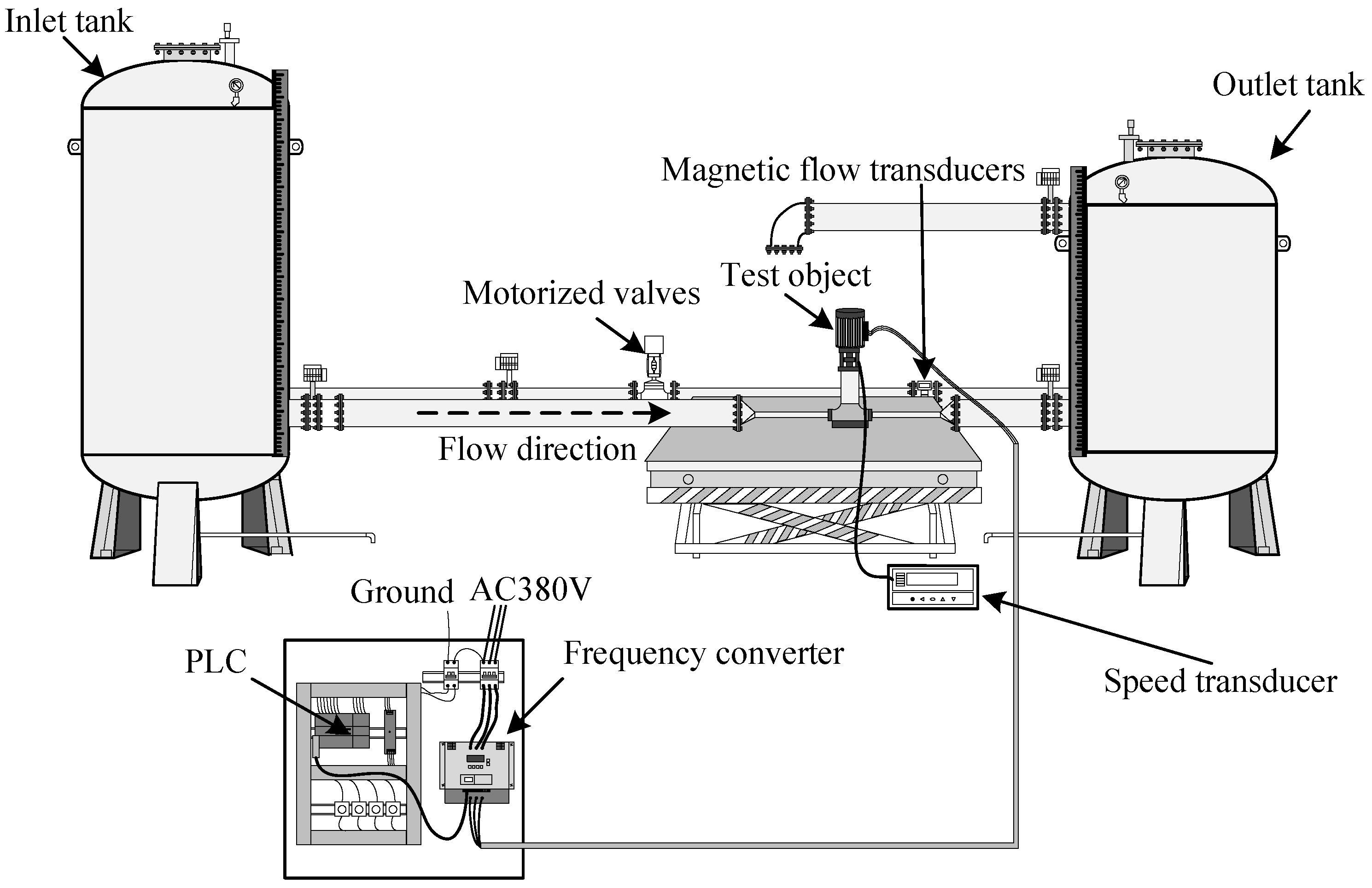
2. Experimental Setup

We measured the test data in a pump closed-loop test facility. It consists of an inlet tank (Yongli, Beichen, Tianjin, China, 2019), an outlet tank (Yongli, Beichen, Tianjin, China, 2019), electric valves (Dunbang, Songjiang, Shanghai, China, 2019), electromagnetic flow meters (Endress + Hauser, Minhang, Shanghai, China, 2019), pressure sensors (Endress + Hauser, Minhang, Shanghai, China, 2019), an electrical control cabinet (Ganlang, Wenzhou, Zhejiang, China, 2019), and a computer (Hasee, Shenzhen, Guangzhou, China, 2021) (see Figure 1). Figure 2 presents the configuration of the test equipment, and Table 1 shows the technical parameters of the measurement instruments.
The test object is a multistage centrifugal pump (Nanyuan, Hangzhou, Zhejiang, China, 2019) with a 5.5 kW induction motor (Nanyuan, Hangzhou, Zhejiang, China, 2019). The nominal operating point is Qnom = 15 m3/h, Hnom = 70.5 m, and nnom = 2900 rpm. The frequency converter (Siemens, Berlin, Brandenburg, Germany, 2020) adjusts the speed of the pump, and a motorized valve controls the flow rates of the pump. The controller is a Siemens S7-200smart ST30 (Siemens, Berlin, Brandenburg, Germany, 2020), and the analog signals are collected through the expansion module Siemens EM AM06 (Siemens, Berlin, Brandenburg, Germany, 2020). The frequency converter communicates with the PLC through the Modbus protocol. The software was written in LabVIEW (Version 18.0, National Instruments, Austin, Texas, United States, 2021), and the PLC communicates with the computer through Ethernet.
To reduce measurement errors, we repeated the test five times and recorded the measured data. Furthermore, we used the average of five experiments as the final data to enhance the reliability of the data.

3. Estimation Methods

3.1. QP Method

The QP and QH curves, typically determined at the nominal speed of the pump, are transformed into the current rotational speed by the affinity law shown in Equations (1)–(3).
Q Q n o m = N N n o m ,
H H n o m = ( N N n o m ) 2 ,
P P n o m = ( N N n o m ) 3 ,
where N is the actual speed, rpm; nnom is the rated speed, rpm; Q is the actual flow rate, m3/h; Qnom is the rated flow rate, m3/h; H is the actual head, m; Hnom is the rated head, m; P is the actual power, kW; Pnom is the rated power, kW.
As shown in Figure 3, in the current QP and QH curves transformed by the affinity law, the flow rate Qest can be calculated using the motor shaft power Pact, and then the head Hest can be computed by the above flow rate Qest. In the QP method, the transformation of the QP curve based on the motor speed and the calculation of the flow rate using the shaft power are two of the critical steps. Hence, the speed and shaft power of the centrifugal pump are vital variables in the flow rate prediction process.

3.2. PN Curves Interpolation Method

As seen in Figure 4a, it is evident that changing the valve opening has a more significant effect on the shaft power of systems with high input frequencies than those with low input frequencies. As the input frequency is 25 Hz, the variation of shaft power is already very tiny. Figure 4b indicates the flow rate variation with valve opening. Changing the valve opening has a more significant effect on the flow rate for systems with a high input frequency than those with a low input frequency. Meanwhile, when the valve opening is small, changing the valve opening has a more significant impact on the flow rate of the centrifugal pump compared to a large valve opening. When the input frequency is 50 Hz, the speed varies by 40 rpm. However, when the input frequency is 25 Hz, the motor speed varies by merely 3 rpm, which demonstrates that the motor speed affected by the valve opening is consistent with the motor shaft power and the pump flow rate (see Figure 5).
We know the QP characteristic curve only reflects the shaft power and flow rate change and indirectly reflects the motor speed change. The affinity law usually assumes that the pump’s efficiency remains constant when transforming the QP curve, which is not affected by changes in motor speed [15]. However, it cannot ignore the effect on pump efficiency and shaft power when the motor speed changes on a large scale. This is a critical factor that affects the prediction accuracy of the QP method.
Therefore, this paper proposed a curve based on motor speed and shaft power, which can visually reflect the variation of motor speed, power, and flow rate. After setting the input frequency, we obtained the speed and power data of different flow rates by changing the valve opening, and then those data were fitted to a PN curve for the same flow rate at different input frequencies. Figure 6a shows that at a specific flow rate, the power increases as the pump speed increases; at a specific speed, the flow rate increases with the power; at a specific power, the flow rate decreases with speed.
As shown in Figure 6b, the Q0 and Qn PN curves divided the graph into three parts. Q0 is the PN curve with the lowest flow rate, generally taken as 0 m3/h. Therefore, when the centrifugal pump works below the Q0 curve, namely the S1 region, the estimation flow rate is 0 m3/h.
The S2 region contains a lot of PN curves, the flow rate from Q0, Q1,… Qj, Qj+1,… Qk−1, Qk covers a wide range of centrifugal pumps with small flow rates, rated conditions, and high flow rates. If t lies between the Qj and Qj+1 flow curves in the S2 region, the flow rate at point t (Nt, Pt) can be obtained by the internal interpolation method, which is shown in Equation (4).
Q e s t = Q j + P t f j ( N t ) f j + 1 ( N t ) f j ( N t ) ( Q j + 1 Q j ) ,
where fj is the power–speed function at the flow rate Qj, and fj+1 is the power–speed function at the flow rate Qj+1.
The S3 region represents the centrifugal pump working above the Qn curve. Typically, pumps operate in the S2 and S1 regions. When the valve opening of the system is so large that the pump is in extreme operating condition, the flow rates are in the S3 region. This paper provides an external interpolation method to calculate the flow rates in the S3 region, as shown in Equation (5).
Q e s t = Q k + P t f k ( N t ) f k ( N t ) f k 1 ( N t ) ( Q k Q k 1 ) ,
where fk−1 is the power–speed function at the flow rate Qk−1, and fk is the power–speed function at the flow rate Qk.

3.3. Estimation Model Based on PN Curves

Figure 7 presents the power variations ΔP of each 2 m3/h flow rate at 50 Hz in the QP curve. As the flow rate increases, dP/dQ gradually decreases, causing ΔP to be smaller. The QP curves for the other input frequencies have similar power variations to 50 Hz. This means that to make the power difference between PN curves approximately equivalent, the flow rate difference between adjacent PN curves should be increased appropriately while in the high flow rate region.
The input frequencies of 50 Hz, 45 Hz, 40 Hz, 35 Hz, and 30 Hz are fitted to the curves with flow rates of Q0 = 0 m3/h, Q1 = 3 m3/h, Q2 = 6 m3/h, Q3 = 9 m3/h, Q4 = 15 m3/h, and Q5 = 21 m3/h. The fitted equations are shown in Equations (6)–(11).
Q 0 :   P = 0.57482 0.000915212 N + 0.000000453394 N 2 ,
Q 1 :   P = 0.60412 0.00105 N + 0.000000704725 N 2 ,
Q 2 :   P = 0.53861 0.000886451 N + 0.000000513669 N 2 ,
Q 3 :   P = 0.63796 0.001 N + 0.000000615403 N 2 ,
Q 4 :   P = 0.88357 0.00105 N + 0.000000952153 N 2 ,
Q 5 :   P = 1.82773 0.00256 N + 0.00000125039 N 2 .
Figure 8 presents the fitted PN curves at different flow rates, and the relevant results of each curve are shown in Table 2. The coefficient of determination R2 of all six fitted curves is close to 1, and the residual sum of squares (RSS) is close to 0, which indicates that the six curves have high accuracy and the results are reliable.
Figure 9 presents the flow chart of the prediction model. For instance, the first step is to obtain a large amount of experimental data of shaft power P, speed N, and flow rate Q by adjusting the input frequency and changing the valve opening, then organizing the data into PN curves with appropriate flow rates. The second step is to collect the shaft power P and speed N of the centrifugal pump and calculate the power P0, P1, P2, P3, P4, and P5 of curves Q0, Q1, Q2, Q3, Q4, and Q5 at different speeds. The flow rate of the centrifugal pump is obtained from the collected power and the calculated power. For instance, the predicted flow rate Qest = 0 m3/h when PP0; when PjPPj+1, the flow rate can be calculated by the internal interpolation method; when PP5, the flow rate can be calculated by external interpolation method.

4. Influence Factors on the Estimation Accuracy
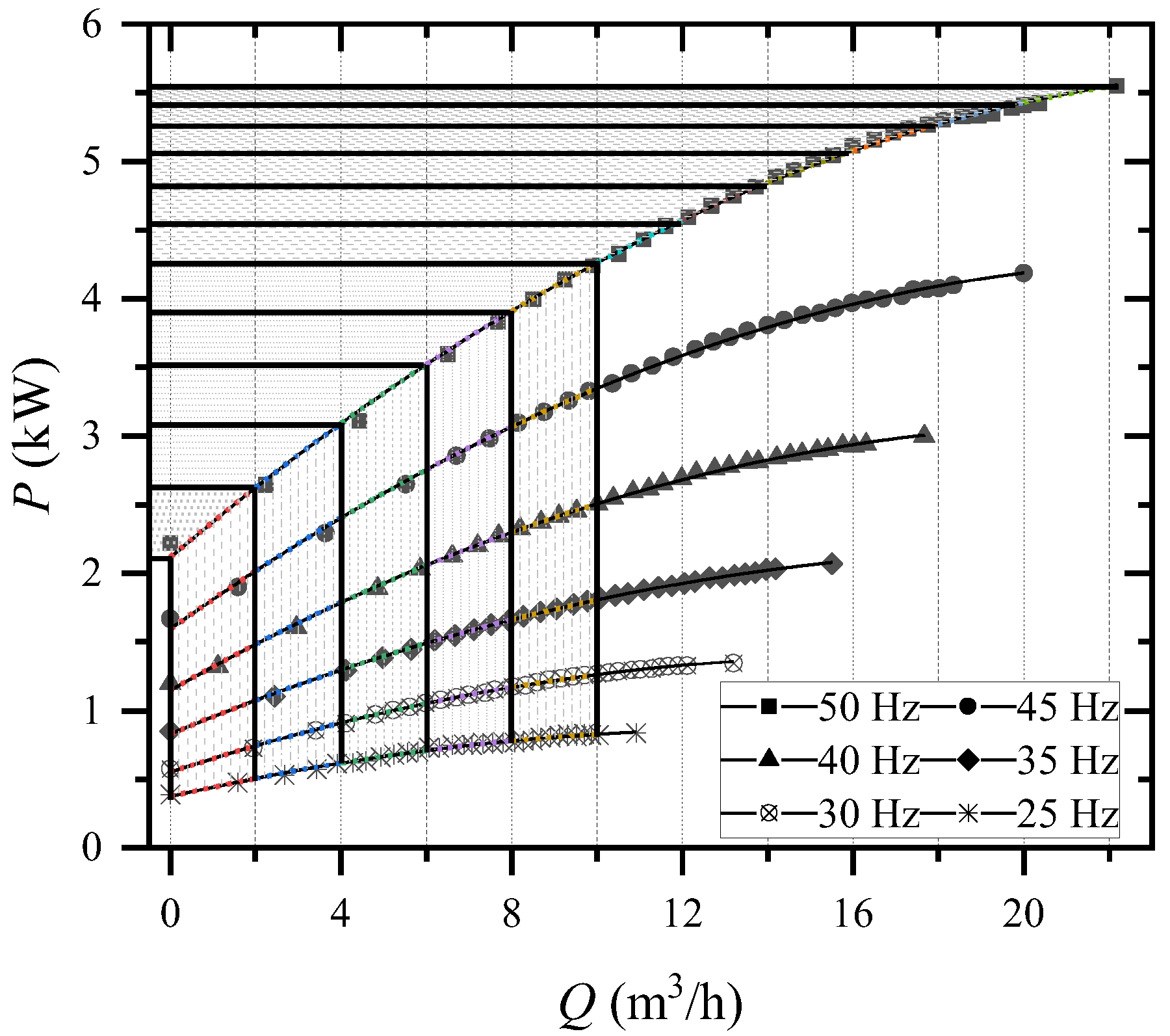
4.1. PN Curves

The PN curves fitted by limited working points somehow deviated from the actual PN curves, which would lead to erroneous estimates of the pumps’ flow rate. At the same time, the difference in flow rates of adjacent PN curves will also affect the prediction results. In addition, the location of the centrifugal pump operating point affects the prediction results. In Figure 10, we assumed that the shaft power of the motor produces ΔP fluctuations. The error in its flow prediction is more than 6 m3/h in area A of the PN curve because the curve in this area is relatively dense, which means that the power variation of the adjacent PN curve is slight. When the pump operates in area B, the error in its flow prediction is between 3 and 6 m3/h. When the pump works in area C, the error in its flow prediction is smaller than 3 m3/h, where the curve is sparse, and the power of the adjacent PN curve varies widely. It indicates that centrifugal pumps operating in the low-speed region are more sensitive to power variations. Therefore, the location of the centrifugal pump’s operating point significantly influences the prediction results.

4.2. Impact of Shaft Power

In addition to the PN curve, the fluctuation of the motor shaft power can change the estimation flow rate. Hence, it also impacts the prediction results. We recorded the motor shaft power fluctuations 50 times at 50 Hz, 45 Hz, 40 Hz, 35 Hz, and 30 Hz and adjusted the valve to set the flow rate at 0 m3/h, 9 m3/h, and 18 m3/h, respectively. As shown in Figure 11, the fluctuation of motor shaft power is more significant at high input frequencies than at low input frequencies. However, the prediction results are less affected by power fluctuations when the input frequency is high since the PN curves of the centrifugal pump are sparse in this region (see Figure 8). Meanwhile, motor shaft power fluctuates slightly at the lower speed operating area where the PN curve is dense. Therefore, the impact of power fluctuations is also insignificant at low input frequencies.
Fluctuations in motor speed also impact the prediction. However, this impact is pretty small and much lower than the impact of shaft power fluctuations. Therefore, it is not discussed in this paper.

5. Results and Discussion

We measured the flow rates at input frequencies of 46 Hz, 41 Hz, 36 Hz, and 31 Hz and compared them with the predictive flow rates to verify the accuracy of the PN curves interpolation method. Meanwhile, we also provided the predictive flow rates using the QP method [14] and the BPNN method [23]. The PN curves interpolation method is more accurate than other methods regardless of the input frequency of 46 Hz, 41 Hz, 36 Hz, or 31 Hz (see Figure 12).
The horizontal and vertical axes of Figure 13 show the measured and predicted flow rates, respectively. The closer the points in the graph are to the line y = x, the closer the predicted flow is to the measured flow. Whether the flow rate is small or large, the point from the PN curves interpolation method is always the closest distance to the line y = x, which indicates that the PN curve interpolation method can better predict the flow rate (see Figure 13).
Figure 14 presents the absolute and relative errors of the three methods, and the specific data are shown in Table 3. The mean absolute error of the interpolation method is 0.1756 m3/h, which is much lower than the other two prediction methods. Meanwhile, the mean relative error of the interpolation method is 2.6919%, while the mean relative error of BPNN and QP prediction methods is 16.6261% and 23.3509%, both of which are much higher than the relative error of the interpolation method. This indicates that the PN curve interpolation prediction method is more accurate and stable.
The QP curve method has nice applications for flow prediction, but the affinity law, which is an important basis of the QP curve method, is not applicable when the speed difference is large [16]. The BPNN flow prediction model is proposed without considering the applicability of the affinity law. Therefore, the BPNN model has higher accuracy than the QP model, as we can see from Figure 12, since even a slight deviation in power can cause significant errors in the flow rate prediction of BPNN. We propose an interpolation method based on the PN curves. The influence of power deviation is reduced by interpolation of the two PN curves in the calculation of the flow rate, as shown in Figure 6. Therefore, the interpolation method based on the PN curves has the highest consistency with the measurement results than the other two methods.

6. Application of the PN Curves Interpolation Method

A validation test was run in a closed centrifugal pump system to verify the applicability of the PN curves interpolation method. We controlled the pump’s flow rate through the valve and frequency converter, and the controller transmitted the speed and power of the motor to the host software via Ethernet. Then, the flow rate was calculated by the PN curve interpolation method programmed into the software. Figure 15 presents the PN curve interpolation method, accurately predicting the flow rates under different input frequencies and valve openings. To determine whether the centrifugal pump works at low or high flow conditions, the points derived from the prediction model are distributed on the line y = x, which indicates that the flow rate of the centrifugal pump can be well predicted based on the PN curves interpolation method (see Figure 16 and Figure 17).

7. Conclusions

This paper proposed a flow rate prediction model based on the PN curve interpolation method. The factors affecting the accuracy of the estimation method were analyzed. Three different estimation models were compared, and the feasibility of this method was verified through experiments. The following conclusions were drawn:
(1)
The PN curves containing speed, power, and flow information were presented, and an interpolated flow prediction model based on these curves was established. The factors affecting the accuracy of the estimation method were analyzed, which mainly include the flow rate and accuracy of the PN curve, the location of the centrifugal pump operational point, and the fluctuation of the shaft power. Particularly in this aspect of the location of the centrifugal pump operational point, centrifugal pumps operating at a low speeds were more sensitive to power variations. Furthermore, the fluctuation of the motor shaft power can cause variations in the estimation flow rate.
(2)
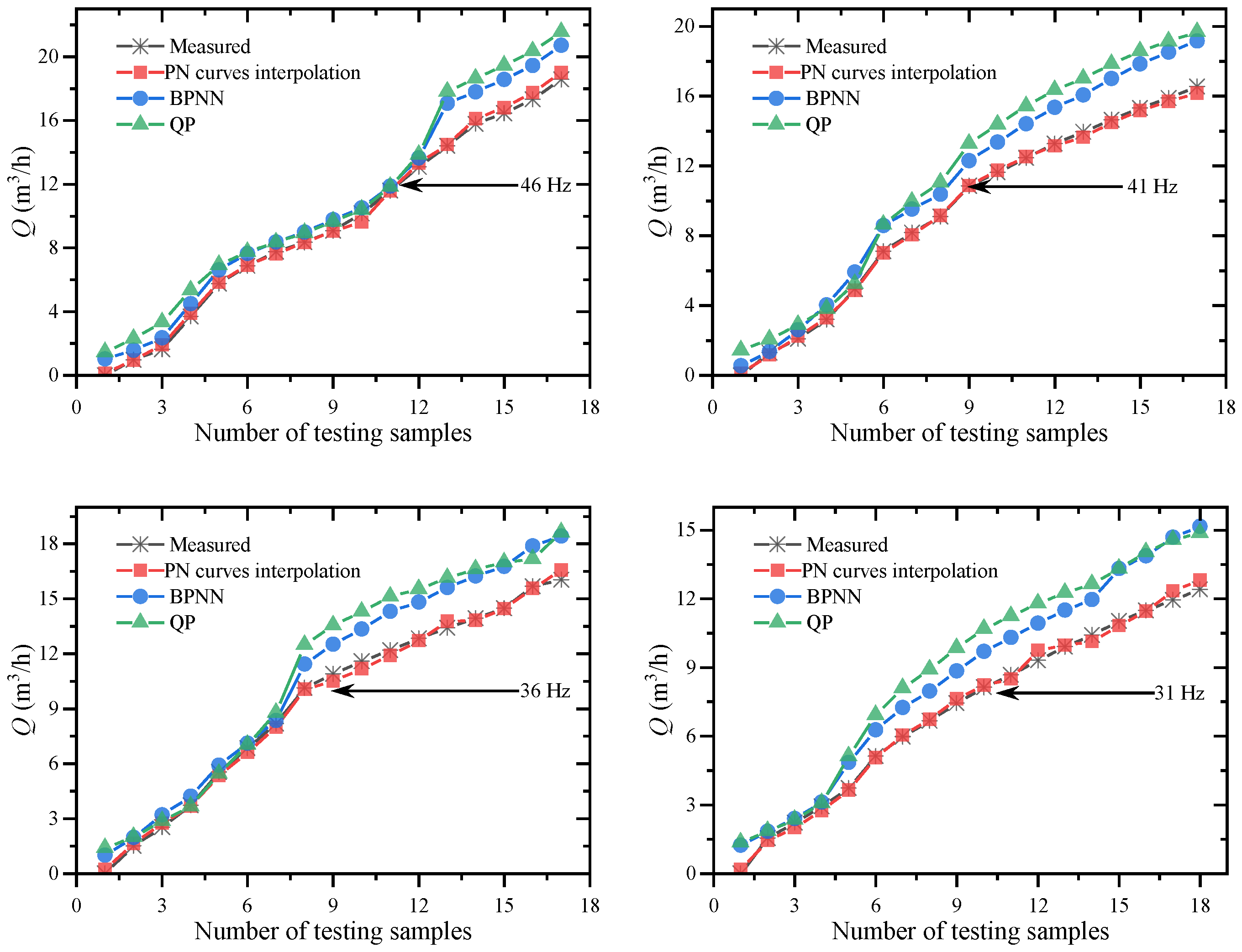
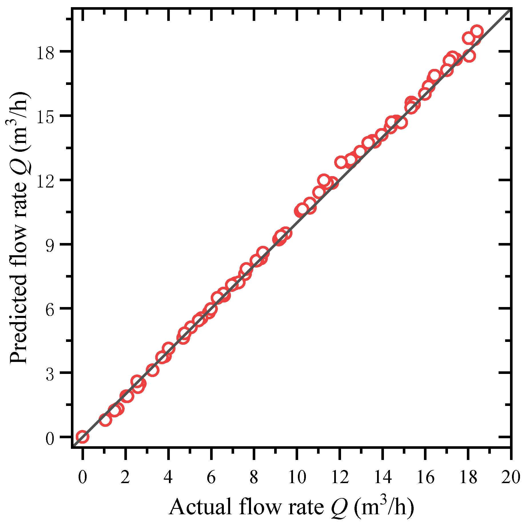
Three different estimation models were compared. The average absolute and relative errors of the interpolated flow prediction method are 0.1756 m3/h and 2.6919%, compared to 1.3851 m3/h and 6.6261% for BPNN and 1.8315 m3/h and 23.35089% for the QP method. This means that the PN curve interpolation method has high accuracy in estimating the flow rates.
(3)
The PN curve interpolation method was tested in an industrial application, and its average absolute errors at 47.5 Hz, 42.5 Hz, 37.5 Hz, and 32.5 Hz are 0.1442 m3/h, 0.2047 m3/h, 0.2197 m3/h, and 0.1979 m3/h, and its average relative errors are 2.0816%, 3.2875%, 3.6981%, and 2.9419%. This highly accurate prediction capability fully meets the monitoring and control requirements and improves the accuracy of centrifugal pump flow prediction at small flow rates.

Author Contributions

Conceptualization, Y.W.; methodology, Y.W.; software, M.F.; validation, D.W. and Y.G.; formal analysis, G.X.; investigation, D.W.; resources, J.M.; data curation, Y.G.; writing—original draft preparation, Y.G.; writing—review and editing, D.W.; visualization, M.F.; supervision, J.M.; project administration, D.W.; funding acquisition, D.W. All authors have read and agreed to the published version of the manuscript.

Funding

This research was funded by the Natural Science Foundation of Zhejiang Province, grant number LGG21E090002, the China Postdoctoral Science Foundation, grant number 2021M691383, and the Science and Technology Program of Zhejiang Province, grant number 2021C01052.

Informed Consent Statement

Not applicable.

Data Availability Statement

Not applicable.

Conflicts of Interest

The authors declare no conflict of interest.

References

  1. De Almeida, A.; Fong, J.; Brunner, C.; Werle, R.; Van Werkhoven, M. New technology trends and policy needs in energy efficient motor systems—A major opportunity for energy and carbon savings. Renew. Sustain. Energy Rev. 2019, 115, 109384. [Google Scholar] [CrossRef]
  2. Torregrossa, D.; Capitanescu, F. Optimization models to save energy and enlarge the operational life of water pumping systems. J. Clean. Prod. 2018, 213, 89–98. [Google Scholar] [CrossRef]
  3. Wang, Z.; Qian, Z.; Lu, J.; Wu, P. Effects of flow rate and rotational speed on pressure fluctuations in a double-suction centrifugal pump. Energy 2018, 170, 212–227. [Google Scholar] [CrossRef]
  4. Goman, V.; Oshurbekov, S.; Kazakbaev, V.; Prakht, V.; Dmitrievskii, V. Energy Efficiency Analysis of Fixed-Speed Pump Drives with Various Types of Motors. Appl. Sci. 2019, 9, 5295. [Google Scholar] [CrossRef] [Green Version]
  5. Oshurbekov, S.; Kazakbaev, V.; Prakht, V.; Dmitrievskii, V.; Gevorkov, L. Energy Consumption Comparison of a Single Variable-Speed Pump and a System of Two Pumps: Variable-Speed and Fixed-Speed. Appl. Sci. 2020, 10, 8820. [Google Scholar] [CrossRef]
  6. Capurso, T.; Bergamini, L.; Torresi, M. A new generation of centrifugal pumps for high conversion efficiency. Energy Convers. Manag. 2022, 256, 115341. [Google Scholar] [CrossRef]
  7. Shankar, V.K.A.; Umashankar, S.; Paramasivam, S.; Hanigovszki, N. A comprehensive review on energy efficiency enhancement initiatives in centrifugal pumping system. Appl. Energy 2016, 181, 495–513. [Google Scholar] [CrossRef]
  8. Viholainen, J.; Tamminen, J.; Ahonen, T.; Ahola, J.; Vakkilainen, E.; Soukka, R. Energy-Efficient Control Strategy for Variable Speed-Driven Parallel Pumping Systems. Energy Effic. 2013, 6, 495–509. [Google Scholar] [CrossRef]
  9. Gu, Y.; Zhang, J.; Yu, S.; Mou, C.; Li, Z.; He, C.; Wu, D.; Mou, J.; Ren, Y. Unsteady Numerical Simulation Method of Hydrofoil Surface Cavitation. Int. J. Mech. Sci. 2022, 228, 107490. [Google Scholar] [CrossRef]
  10. Luna, T.; Ribau, J.; Figueiredo, D.; Alves, R. Improving Energy Efficiency in Water Supply Systems with Pump Scheduling Optimization. J. Clean. Prod. 2019, 213, 342–356. [Google Scholar] [CrossRef]
  11. Lindstedt, M.; Karvinen, R. Optimal Control of Pump Rotational Speed in Filling and Emptying a Reservoir: Minimum Energy Consumption with Fixed Time. Energy Effic. 2016, 9, 1461–1474. [Google Scholar] [CrossRef]
  12. Luo, Y.; Zhixiang, X.; Sun, H.; Yuan, S.; Yuan, J. Research on the Induction Motor Current Signature for Centrifugal Pump at Cavitation Condition. Adv. Mech. Eng. 2015, 7, 708902. [Google Scholar] [CrossRef] [Green Version]
  13. Benlaloui, I.; Drid, S.; Chrifi-Alaoui, L.; Ouriagli, M. Implementation of a New MRAS Speed Sensorless Vector Control of Induction Machine. IEEE Trans. Energy Convers. 2015, 30, 588–595. [Google Scholar] [CrossRef]
  14. Hammo, S.; Viholainen, J. Providing Flow Measurement in Parallel Pumping Systems from Variable Speed Drives. World Pumps 2006, 2006, 30–33. [Google Scholar] [CrossRef]
  15. Ahonen, T.; Tamminen, J.; Ahola, J.; Viholainen, J.; Aranto, N.; Kestilä, J. Estimation of pump operational state with model-based methods. Energy Convers. Manag. 2010, 51, 1319–1325. [Google Scholar] [CrossRef]
  16. Ahonen, T.; Tamminen, J.; Ahola, J.; Kestila, J. Frequency-Converter-Based Hybrid Estimation Method for the Centrifugal Pump Operational State. IEEE Trans. Ind. Electron. 2011, 59, 4803–4809. [Google Scholar] [CrossRef]
  17. Tamminen, J.; Viholainen, J.; Ahonen, T.; Ahola, J.; Hammo, S.; Vakkilainen, E. Comparison of Model-Based Flow Rate Estimation Methods in Frequency-Converter-Driven Pumps and Fans. Energy Effic. 2014, 7, 493–505. [Google Scholar] [CrossRef] [Green Version]
  18. Ahonen, T.; Tamminen, J.; Ahola, J.; Niinimaki, L.; Tolvanen, J. Sensorless estimation of the pumping process characteristics by a frequency converter. In Proceedings of the 15th European Conference on Power Electronics and Applications (EPE), Lille, France, 3–5 September 2013; pp. 1–10. [Google Scholar] [CrossRef]
  19. López-Lineros, M.; Estévez, J.; Giráldez, J.V.; Madueño, A. A New Quality Control Procedure Based on Non-Linear Autoregressive Neural Network for Validating Raw River Stage Data. J. Hydrol. 2014, 510, 103–109. [Google Scholar] [CrossRef]
  20. Claveria, O.; Torra, S. Forecasting Tourism Demand to Catalonia: Neural Networks vs. Time Series Models. Econ. Model. 2014, 36, 220–228. [Google Scholar] [CrossRef]
  21. Wu, Q.; Shen, Q.; Wang, X.; Yang, Y. Estimation of Centrifugal Pump Operational State with Dual Neural Network Architecture Based Model. Neurocomputing 2016, 216, 102–108. [Google Scholar] [CrossRef]
  22. Han, W.; Nan, L.; Su, M.; Chen, Y.; Li, R.; Zhang, X. Research on the Prediction Method of Centrifugal Pump Performance Based on a Double Hidden Layer BP Neural Network. Energies 2019, 12, 2709. [Google Scholar] [CrossRef] [Green Version]
  23. Kong, X.; Ma, S.; Ma, T.; Li, Y.; Cong, X. Mass Flow Rate Prediction of Direct-Expansion Solar-Assisted Heat Pump Using R290 Based on ANN Model. Sol. Energy 2021, 215, 375–387. [Google Scholar] [CrossRef]
  24. Wu, D.; Huang, H.; Qiu, S.; Liu, Y.; Wu, Y.; Ren, Y.; Mou, J. Application of Bayesian Regularization Back Propagation Neural Network in Sensorless Measurement of Pump Operational State. Energy Rep. 2022, 8, 3041–3050. [Google Scholar] [CrossRef]
  25. Luo, H.; Zhou, P.; Shu, L.; Mou, J.; Zheng, H.; Jiang, C.; Wang, Y. Energy Performance Curves Prediction of Centrifugal Pumps Based on Constrained PSO-SVR Model. Energies 2022, 15, 3309. [Google Scholar] [CrossRef]
Figure 1. A closed-loop pump test system.
Processes 10 02163 g001
Figure 2. Experimental facilities: (a) closed-loop test bed, (b) vertical centrifugal pump, and (c) control system.
Processes 10 02163 g002
Figure 3. QP characteristic curve method: (a) QP curves and (b) QH curves.
Processes 10 02163 g003
Figure 4. Shaft power and flow variation with valve opening: (a) shaft power and (b) flow rate.
Processes 10 02163 g004
Figure 5. Speed varies with valve opening.
Processes 10 02163 g005
Figure 6. PN curves and PN curves interpolation methods: (a) PN curves for different flow rates and (b) PN curve-based flow estimation method.
Processes 10 02163 g006
Figure 7. Power variation of QP curve.
Processes 10 02163 g007
Figure 8. PN curves.
Processes 10 02163 g008
Figure 9. Flow chart of flow rate estimation algorithm.
Processes 10 02163 g009
Figure 10. Variation of estimation for different working points.
Processes 10 02163 g010
Figure 11. Fluctuation of the shaft power.
Processes 10 02163 g011
Figure 12. Comparison of the predictive flow rates of the three methods.
Processes 10 02163 g012
Figure 13. Comparison of the results of the three estimation methods.
Processes 10 02163 g013
Figure 14. Errors of the three estimation methods: (a) absolute errors and (b) relative errors.
Processes 10 02163 g014
Figure 15. Results of flow estimation.
Processes 10 02163 g015
Figure 16. Comparison of predicted and actual flow rates.
Processes 10 02163 g016
Figure 17. Errors of the estimated flow rate: (a) absolute errors and (b) relative errors.
Processes 10 02163 g017
Table 1. Test sensor information.
Sensor TypeMeasurement RangePrecisionManufacturers
Electromagnetic flowmeter0–150 m3/h0.2%Endress + Hauser, Switzerland
Power meterCurrent, voltage, power0.5%Qingzhi instrument, China
Tachometer0–20,000 rpm±1 rpmOnosokki, Japan
Table 2. Curve fitting results.
ItemsQ0Q1Q2Q3Q4Q5
R20.99990.99990.999990.9999610.99994
RSS1.465 × 10−41.051 × 10−44.146 × 10−51.716 × 10−42.455 × 10−53.312 × 10⁻⁴
Table 3. Error data of the three estimation methods.
ItemsErrors
MaximumAverageMinimum
PN curves interpolationδ (m3/h)0.54090.17560.0021
ε (%)16.98142.69190.0181
BPNNδ (m3/h)2.75651.38510.0717
ε (%)61.973916.62612.0429
QPδ (m3/h)3.41911.83150.0496
ε (%)137.693623.350891.3291
Publisher’s Note: MDPI stays neutral with regard to jurisdictional claims in published maps and institutional affiliations.

