The Total Low Frequency Oscillation Damping Method Based on Interline Power Flow Controller through Robust Control

Abstract

The interline power flow controller (IPFC) can control the active power and reactive power of different lines in power system. To utilize the flexible control ability of IPFC and increase the damping characteristic of its controller AC system, this paper proposes a low-frequency oscillation (LFO) suppress method through IPFC. The LFO suppress method is designed by adding supplementary signals to the outer current control loop of IPFC. In addition to adding supplementary active power signals, the reactive supplementary signals are also added to related control loop, which is the total control scheme. To obtain the power system’s small signal model, the identification technology based on the PRONY algorithm is used. In addition, the robust control theory is also applied to make the controllers more adaptive. To verify the effectiveness of the proposed method, two controllers including both the active and reactive controllers are designed for in PSCAD software. Furthermore, the simulation results prove the proposed method can reach a better control effect and is also of robustness.

1. Introduction

With the development of power systems and transmission technology, the transmission voltage and distance are much higher and longer than before. The power grid scale is expanded, and the structure is becoming more and more complex. When the characteristic of the modern power system changes, many new challenges show up and threaten the safety operation of the grids [1]. Among these challenges, the lack of transmission capacity of the existing grid is one of the most important problems to be solved. The lack of transmission capacity of the existing grid problem is caused by many reasons. As the power supply bases are often far away from the load center, lots of transmission channels are needed [2]. However, due to the constraints of policies and regulations, environmental protection and costs, the newly proposed power transmission lines have been reduced and limited. Simultaneously, renewable energy’s sharply increasing also makes the traditional transmission line face the power fluctuation pressure [3], such that developing new power transmission technology and increasing existing AC transmission lines’ capacity is the more useful method to improve the large-scale power grid efficiency [4].

Using new technology and equipment to solve the overload problem and make power flow more balance has several ways. The first way is the high-voltage-direct-current transmission (HVDC) technology [5]. The capacity of the HVDC system can be larger than the HVAC system and the distance can also be much longer than a traditional AC line. Especially, the HVDC system can control its active power flexibly such that the transmission channel can be expanded when the power is transferred by DC lines [6]. Furthermore, in the last decades, lots of DC systems have been established. However, the main part of the existing transmission power grid is the AC system, they still suffer from the overload threat when the AC power grid encounter faults [7].

To overcome this problem, lots of flexible AC transmission technologies (FACTS) are also invented. Furthermore, the installation of FACTS devices in the existing power grid structure has become the main means to increase power grid transmission capacity [8]. The advantages of the FACTS devices include continuous and rapid control of AC power flow, provision of reactive power compensation, reduction of power loss, improvement of static and transient stability of power grid, and flexible operation of power grid [9]. At present, the unified power flow controller (UPFC) is recognized as the most advanced and most popular in practical research, development, and engineering application [10]. Specifically, UPFC has a variety of power grid regulation functions, mainly including voltage maintenance, reactive or active power compensation, line impedance compensation, power flow regulation, damping low-frequency oscillation or sub-synchronous resonance, enhancing system power angle and voltage stability, and improving system transient or medium and long-term stability [11]. To better realize the efficient and stable operation of UPFC in the power grid, many experts and scholars have studied the mathematical modeling, operation principle, control strategy, multi-functional regulation efficiency, and oscillation damping effect of UPFC [12].

At the same time, the interline power flow controller (IPFC) is also researched and is the representative device of the third-generation FACTS devices. Different from UPFC, IPFC can control the power flow of multiple transmission channels at the same time, to avoid the risk of other adjacent heavy load lines’ overload when UPFC adjusts the power flow regulation [13]. In addition, even if one IPFC installation line encounters a fault, the other IPFCs can continue to control the system power flow by switching their control mode to avoid the deterioration caused by the fault. Therefore, on lots of practical occasions, IPFC has certain application advantages in power flow regulation compared with UPFC [14].

In addition to the power flow regulation function, the other IPFC control ability is to damp the low-frequency oscillations. Low-frequency Oscillation often occurs in large-scale power systems [15,16], and some researchers have carried out initial work to enhance the dynamic stability of the system and IPFC itself. Reference [17] established the small-signal model of the IPFC and validates it by using detailed electromagnetic transients’ simulation. Using the validated model, the damping capabilities of the IPFC and the UPFC are compared and rationalized. In reference [18] an integrated approach of radial basis function neural network (RBFNN) and Takagi-Sugeno (TS) fuzzy scheme with a genetic optimization of their parameters have been developed in the paper to design intelligent adaptive controllers for improving the transient stability performance of power systems. Furthermore, in reference [19], a fuzzy logic based IPFC damping controller is designed and compared with a conventional damping controller to mitigate the low-frequency oscillations for the multi-machine power system.

Although the above research has researched the damping method of the low-frequency oscillation through IPFC, they usually concentrate on the artificial intelligence method to damp the oscillations. On the other side, the active power control loop is used to damp the oscillation, but the reactive power is always ignored. It is known that the active power is more related to the oscillation problem, but the reactive control channel also has the impact on the damping ratio, which is always ignored when people design the controller. In addition, the IPFC has the ability to control the active and reactive power on the line. To increase the damping characteristic of the AC system, this paper proposes a low-frequency oscillation (LFO) suppress method based on IPFC’s flexible control ability. The LFO suppress method is designed by adding supplementary signals to the outer current control loop of IPFC. In addition to adding supplementary active power signals, the reactive supplementary signals are also added to the corresponding control loop, which is the total control scheme. The novelty of this paper can be summarized as follows.

• The low-frequency oscillation damping controller is designed through IPFC devices, and it validates that IPFC can enhance the dynamic stability of the AC system effectively.
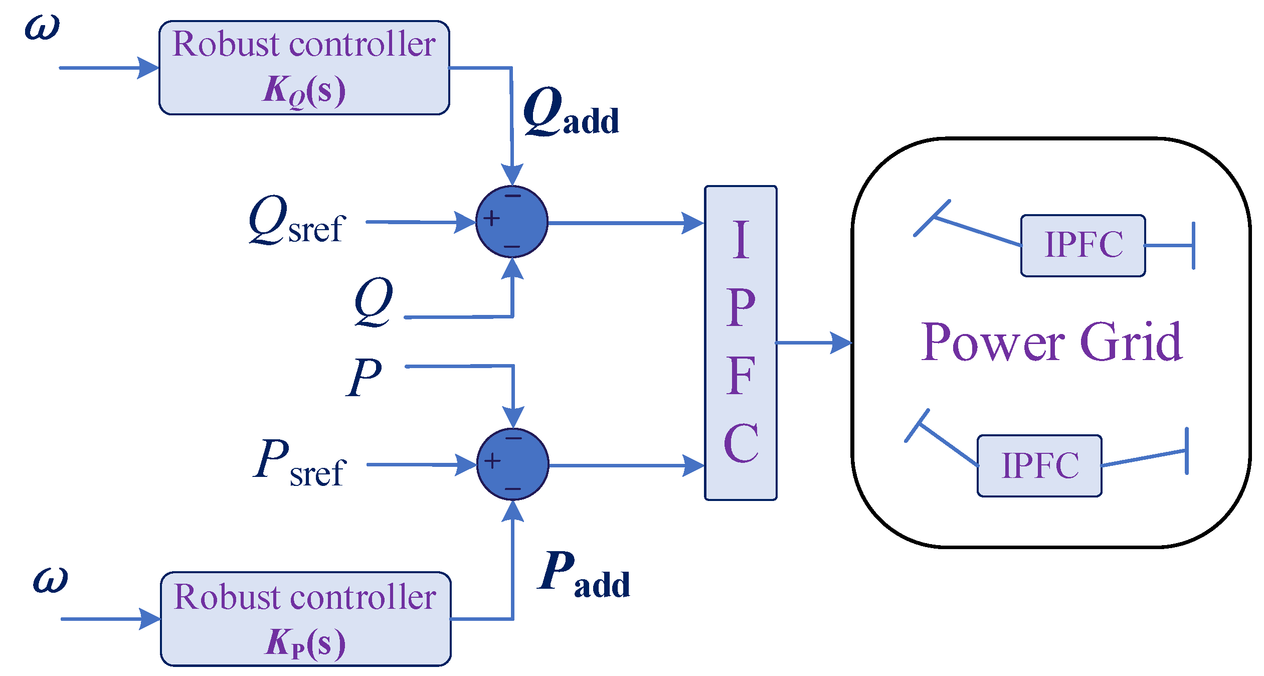
• The total controller is designed through both the active control and reactive control loop of the IPFC. A better control effect and be reached through such strategy, and the damping ability can be guaranteed by the other controller when one controller is in fault.
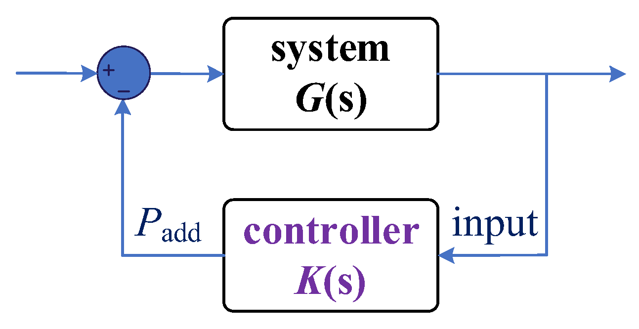
• The robust control theory is used when the damping controller is designed, which can make the control correct and effective on most occasions, even when the system operation mode changes.

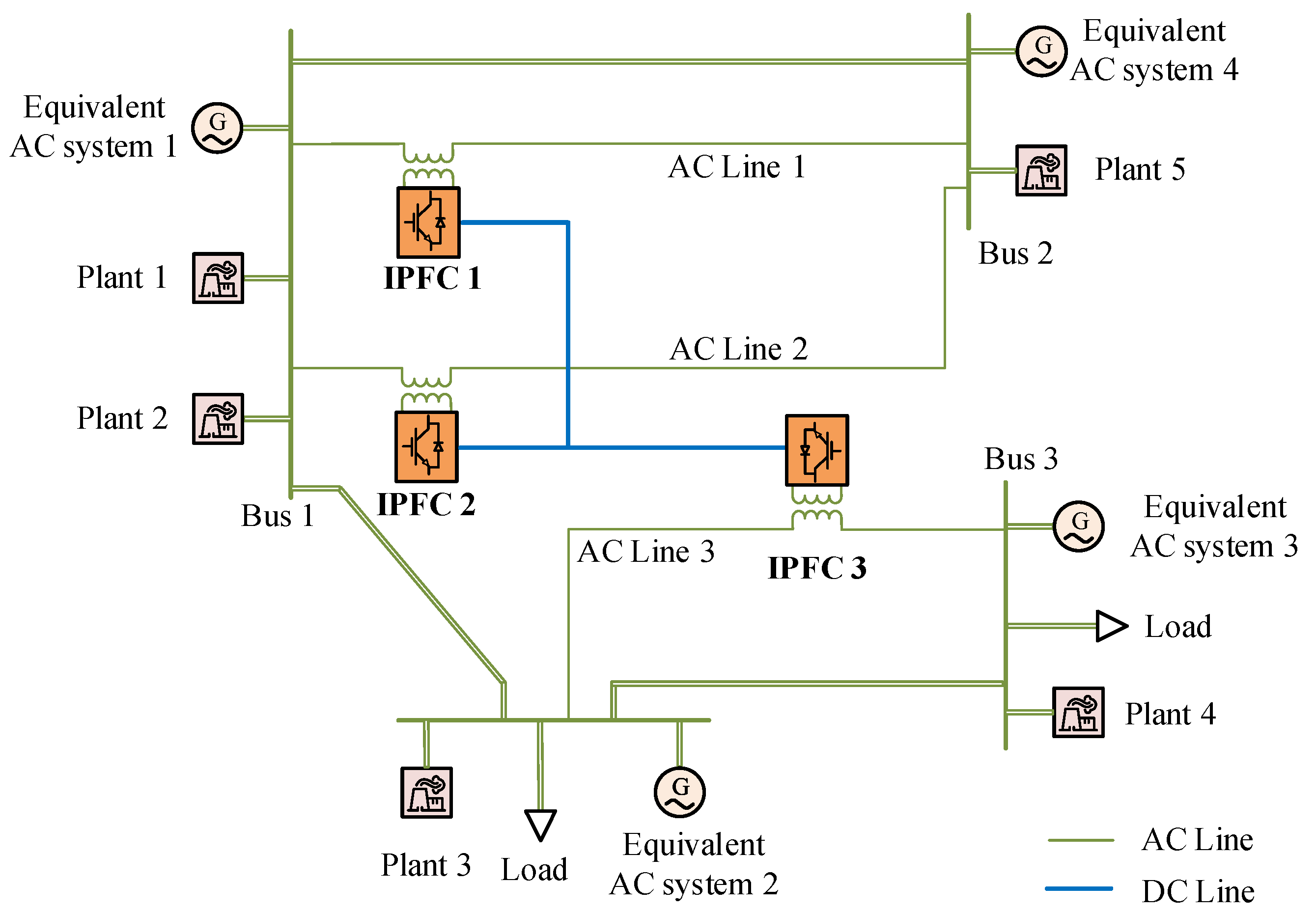
2. The Interline Power Flow Controller

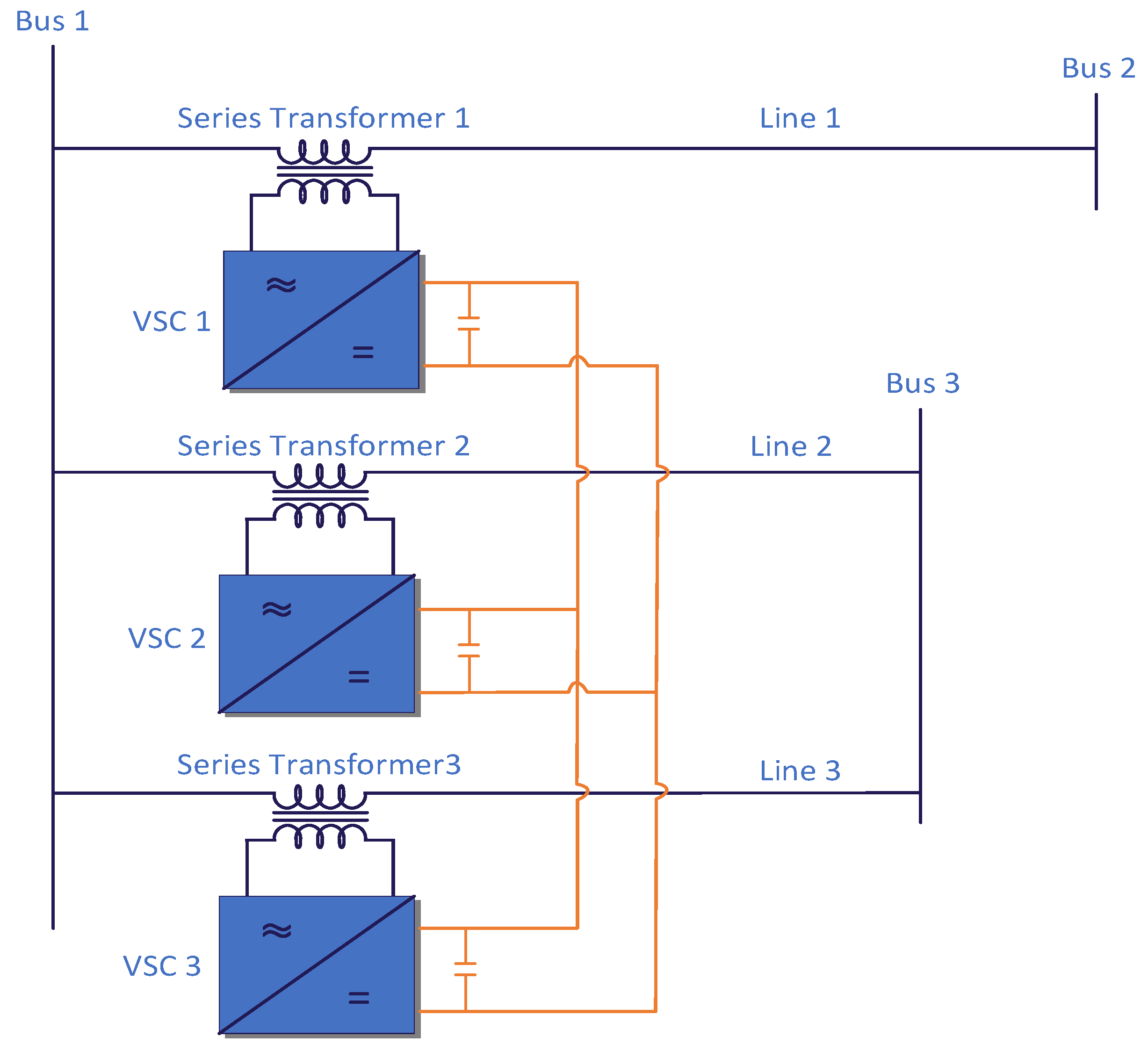
2.1. The Structure of IPFC

Interline power flow controller (IPFC) is one of the most powerful integrated flexible AC transmission systems (FACTS) equipment. Different from the total power flow controller (UPFC), IPFC can realize accurate and flexible power flow control of multiple AC lines at the same time. The IPFC is connected in series with multiple transmission lines, which is based on the series coupled transformer as Figure 1 shows.

Similar to the characteristics of UPFC, the active power interaction between each IPFC converter is in a dynamic balance state, that is, IPFC equipment itself neither absorbs active power nor emits active power. In normal operation, the IPFC-controlled lines can be divided into mainly controlled lines and auxiliary-controlled line. The active power and reactive power of the mainly controlled lines can be controlled, while only the reactive power can be controlled in an auxiliary-controlled line.

Based on such settings of the IPFC, one or several heavy load lines can be selected as the mainly controlled line. Such that the overload power flow can be reasonably allocated to other secondary priority lines. By balancing the power flow of each transmission channel, the power flow overload can be avoided, and the transmission capacity of the system can be greatly improved.

Take the 3-line IPFC in Figure 1 for example, line 1 can be selected as the mainly controlled line, and line 2 and line 3 can be selected as the auxiliary-controlled lines. Such that the active power and reactive power of line 2 and line 3 can be controlled. Furthermore, only the reactive power of line 1 can be controlled as the auxiliary-controlled line is mainly used for maintaining the DC voltage stability.

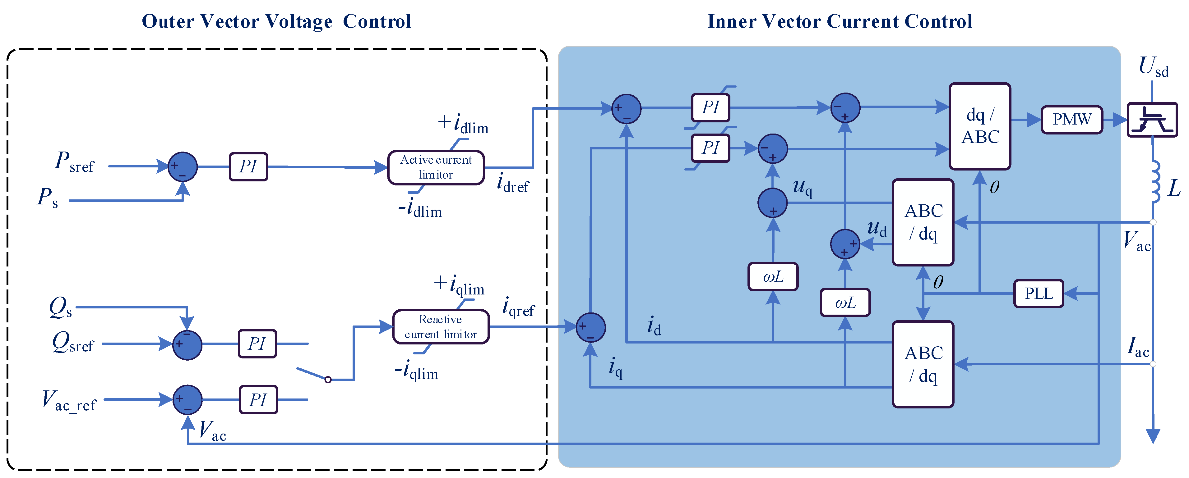
2.2. The Control Strategy of Mainly Controlled Converter

The basic control strategy of IPFC is presented in Figure 2. The control strategy of IPFC is almost the same as the conventional voltage-sourced converter (VSC). The VSC control system based on vector control can be divided into two parts. The first part of the control is the outer vector voltage control part. It determines the actual electrical variables to be controlled. In outer control, the active type of variable and reactive type variables can both be controlled. Specifically, the active type of variable of mainly control converter in IPFC is set as the active power of the controlled line. In addition, the reactive variables to be controlled in mainly control converter can be set as the reactive power of the line and the AC voltage of the line too. For second part of control strategy is the inner vector current control, which has no difference from the VSC inner vector control.

Figure 2 shows the control diagram in detail. Furthermore, the P_sref and the P_s denote the reference and the actual active power of the mainly controlled line, while Q_sref and Q_s denote the reference and the actual reactive power of the mainly controlled line. V_{ac_ref} and V_ac mean the AC voltage’s reference and actual value also. The i_dref is the output of the outer control which is called the active power current. Similarly, i_qref is defined as the reactive power current.

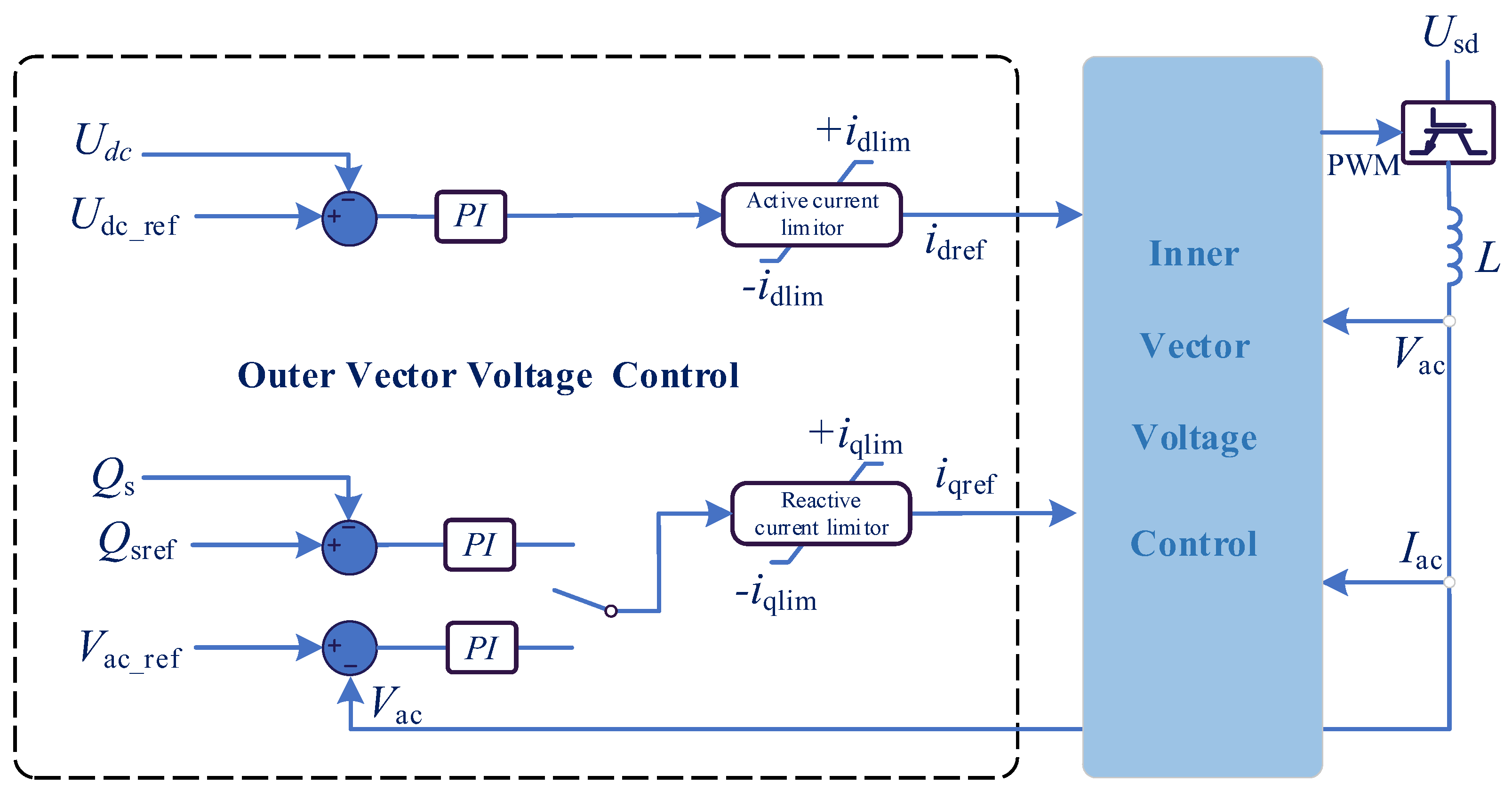
2.3. The Control Strategy of Auxiliary Controlled Converter

The control of the auxiliary controlled converter is presented in Figure 3. It can be seen that the control scheme is basically the same as the mainly controlled converter in IPFC, and the only difference is that the active power control mode is set as DC voltage control in outer vector control. That is because the auxiliary controlled converter needs to keep the DC voltage when the IPFC operation point varies. It means the active power of the auxiliary controlled line cannot be controlled, while the reactive power of the auxiliary controlled line can also be controlled. In Figure 3, U_dc and U_{dc_ref} denote the DC voltage and its reference, respectively. In addition, the inner vector voltage control part is the same as Figure 2 and not be presented for simplification.

3. Total Low Frequency Oscillation Damping Method Based on System Identification

In this part, the total low frequency oscillation damping method will be introduced, which is based on system identification and robust control theory.

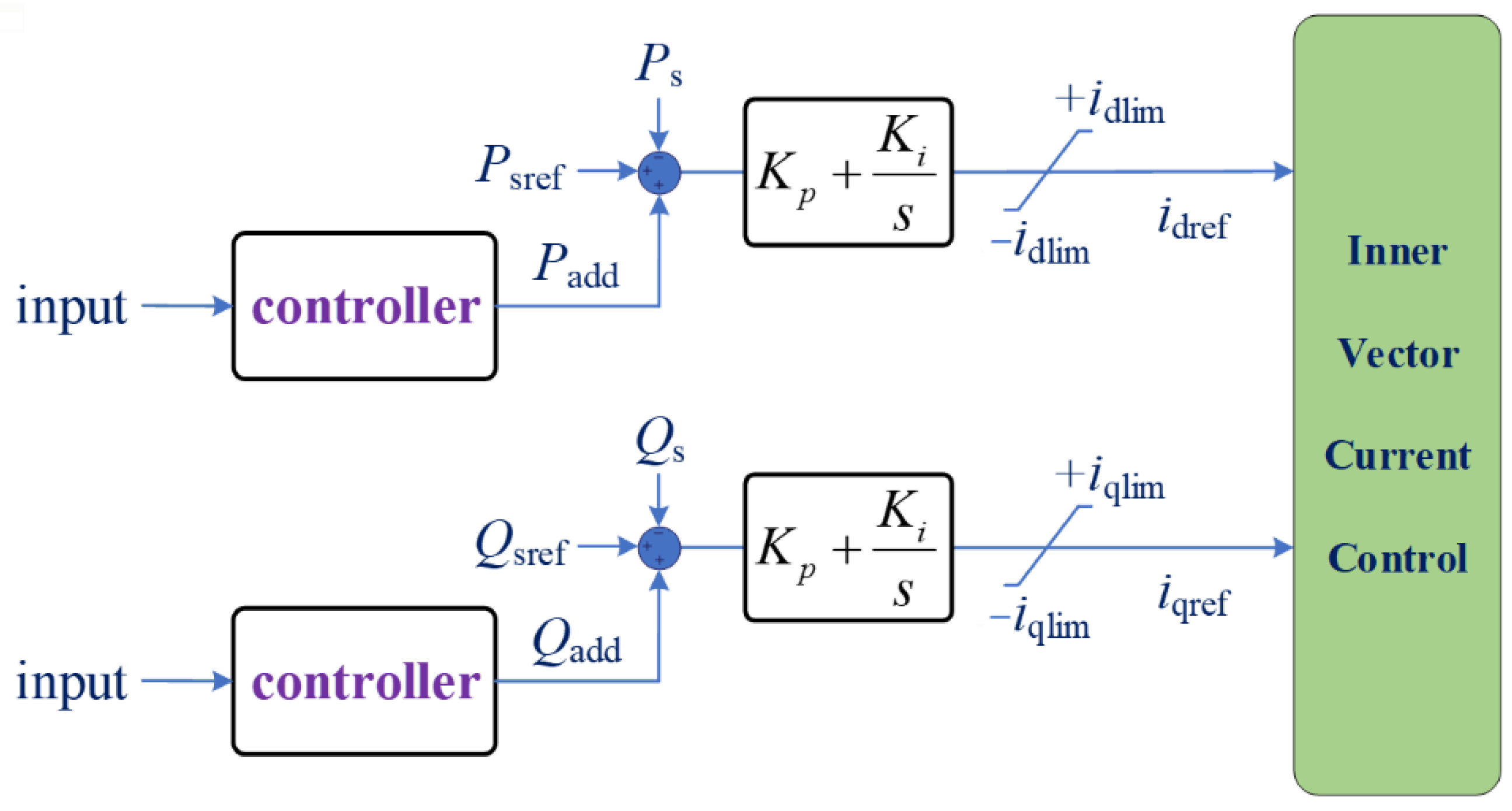
3.1. The Total Damping Strategy for IPFC

As described before, the LFO damping control of IPFC can be designed as it can control the power flow of the AC line. It is known that the converters of IPFC can be divided into mainly controlled converters and the auxiliary controlled converter. Thus, the additional LFO damping controller can be designed for every converter except the active power control loop of the auxiliary controlled converter, because this control channel should be left to the DC voltage control.

On the other side, although the LFO is more related to the active power control channel, the reactive power can influence the oscillations. Thus, the active and reactive power control loops can both be used for damping controllers design, which are the outer current control loop of each IPFC converter specifically. Furthermore, based on such a concept, the control diagrams of a total damping strategy are presented in Figure 4.

3.2. The System Modeling Method Based on PRONY Identification

According to Figure 5, the controller design should obtain the system model. In this paper, the PRONY algorithm is used to identify the system.

The Prony algorithm is widely used in the field of power system analysis and control [20]. Compared with small signal modeling and analysis, the information obtained by Prony algorithm can be more accurate and efficient. Using Prony algorithm to analyze the actual system can directly obtain the key information such as the dominant pole of the system and the residue of the transfer function and so on. The principle of Prony algorithm is to use a reduced order model to approximate the original high-order model of the large-scale system.

Setting Δt is the equal time interval, and N data points can be obtained by sampling. Then the mathematical model is obtained by linear combination simulation of P exponential functions,

$$\begin{array}{c}y(n)\approx \mathit{Z}{\mathit{B}}^T={\displaystyle \sum _{i=1}^p{A}_i}{e}^{j{\theta }_i}\cdot e^{n({\sigma }_i+j2\pi f_i)\Delta t}\\ (n=0,1,\dots ,N-1)\end{array}$$

(1)

where, y(n) indicates the nth sampling point, $\mathit{Z}=[z_1,z_2,\dots ,z_p]$ is the pole array and $\mathit{B}=[b_1,b_2,\dots ,b_p]$ is the residue array correspondingly. In which, A_i is amplitude, θ_i represents the initial phase, σ_i represents the attenuation factor, and f_i represents the frequency. Based on such data, the Y matrix can be constructed according to the sampled data points.

$$\mathit{Y}=\left[\begin{array}{cccc}y(n)& y(n-1)& \cdots & y(0)\\ y(n+1)& y(n)& \cdots & y(1)\\ ⋮& ⋮& ⋮& ⋮\\ y(N-1)& y(N-2)& \cdots & y(N-n-1)\end{array}\right]$$

(2)

Letting $\mathit{Y}{\mathit{A}}^T=0$, we can obtain (3) with the help of (2), in which, $\mathit{A}=[1,a_1,a_2,\dots ,a_p]$.

$$Z^p+a_1{Z}^{p-1}+\cdots +a_{p-1}Z+a_p=0$$

(3)

The polynomial (3) is composed of coefficients. By solving this polynomial, the P poles identified by Prony can be obtained. Next, the least square method is used to solve the Equation (4) to obtain residue B.

$$\left[\begin{array}{cccc}1& 1& \cdots & 1\\ z_1& z_2& \cdots & z_p\\ ⋮& ⋮& ⋮& ⋮\\ z_1^{N-1}& z_2^{N-1}& \cdots & z_p^{N-1}\end{array}\right]\left[\begin{array}{c}{b}_1\\ b_2\\ ⋮\\ b_p\end{array}\right]=\left[\begin{array}{c}y(0)\\ y(1)\\ ⋮\\ y(N-1)\end{array}\right]$$

(4)

Using the calculation results of Equations (3) and (4), the amplitude, phase, attenuation factor and frequency of the linear combination of the analog input signal in Equation (1) can be calculated out through Equation (5).

$$\{\begin{array}{c}{\mathrm{A}}_i=\left|b_i\right|\\ {\theta }_i=\arctan [\mathrm{Im}(b_i)/\mathrm{Re}(b_i)]\\ {\sigma }_i=\mathrm{In}\left|z_i\right|/\Delta t\\ f_i=\frac{\arctan [\mathrm{Im}(z_i)/\mathrm{Re}(z_i)]}{2\pi \Delta t}\end{array}$$

(5)

3.3. The Robust Control LMI Method

To design the controller with satisfied adaptiveness, the robust control theory proposed in [21] is used in this paper. The detailed information can be found in this reference and the final control scheme is shown in Figure 6.

4. Simulation Verifications

The topology of system with IPFC for simulations are presented in Figure 7. In addition, the system parameters can be found in

Table 1. The Control Modes of Each IPFC Converter.

Control Strategy	IPFC1	IPFC2	IPFC3
Control Functions	mainly controlled converter	mainly controlled converter	auxiliary controlled converter
Active power control mode	Constant active power control	Constant active power control	Constant DC voltage control
Reactive power control mode	Constant reactive power control	Constant reactive power control	Constant reactive power control

and

Table 2. System Parameters.

	IPFC1	IPFC2
AC system	Rated AC voltage/kV	380
IPFC Converter	Rated DC voltage/kV	400
	HBSM number	180
	HBSM Capacitance/mF	15
	Arm reactance/mH	50
	idlim of MMC1/p.u.	1.0
	iqlim of MMC1/p.u.	0.4
	idlim of MMC2/p.u.	1.0
	iqlim of MMC2/p.u.	0.4
	idlim of MMC3/p.u.	1.0
	iqlim of MMC3/p.u.	1.0
Line Parameter	Resistance/ohm/m	0.1782 × 10–4
	Inductive Reactance/ohm/m	0.3139 × 10–3
	Capacitive Reactance/Mohm*m	273.5448
	Line 1/km	150
	Line 2/km	150
	Line 3/km	150

.

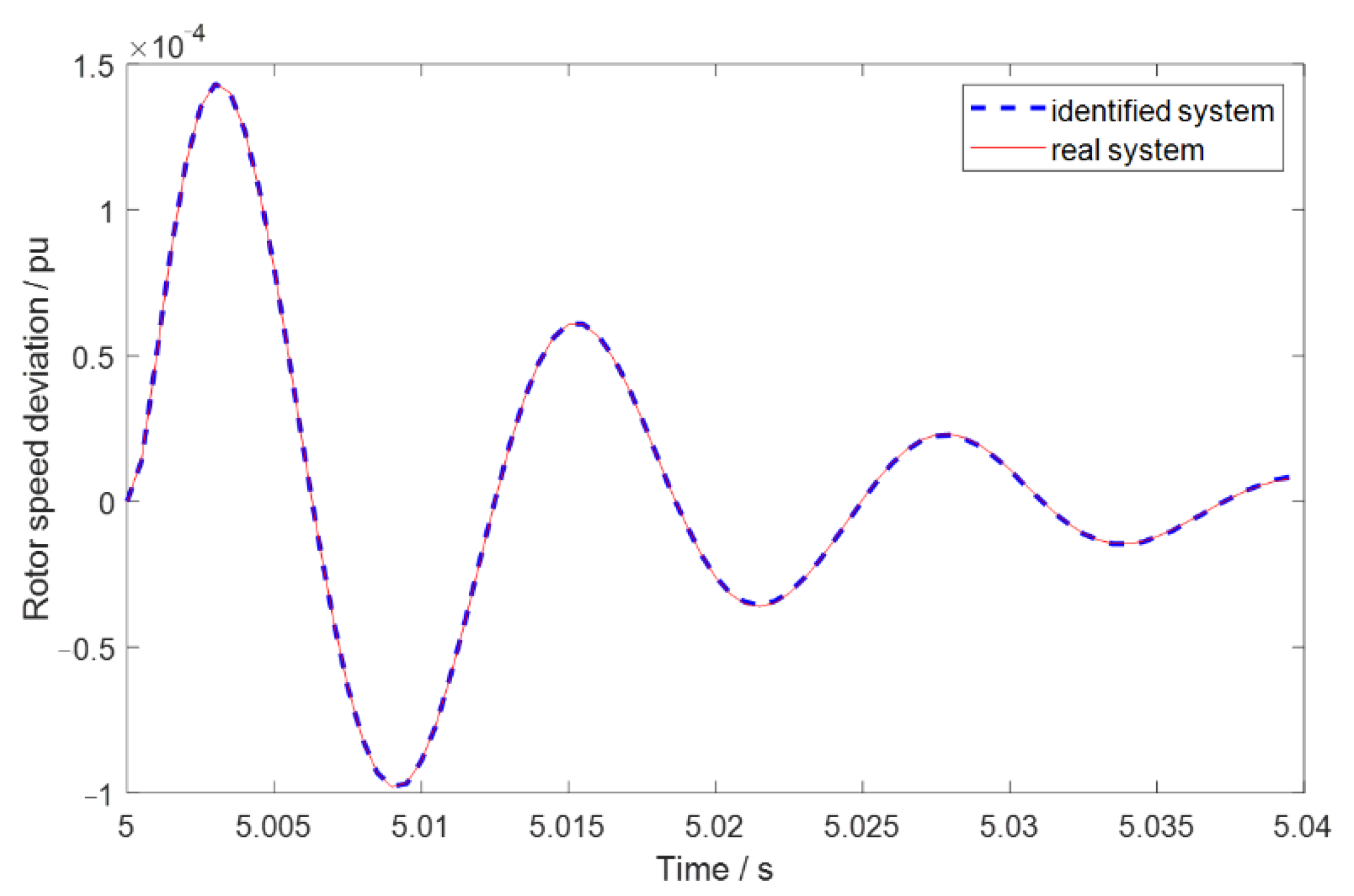
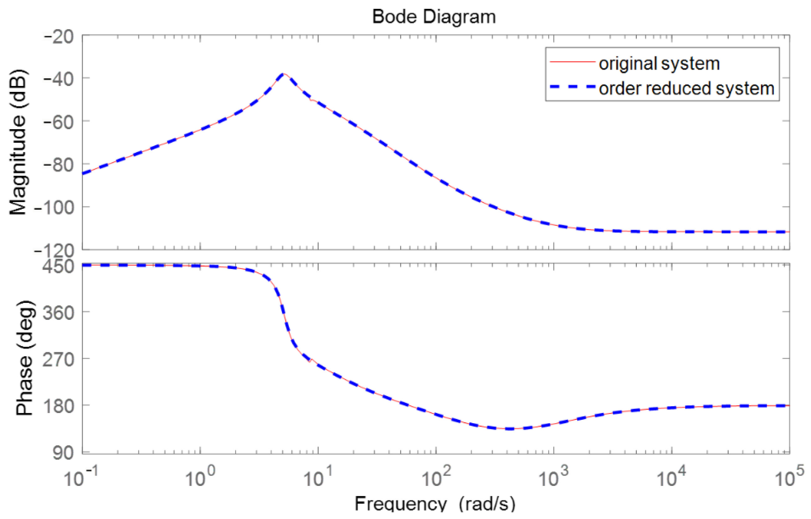
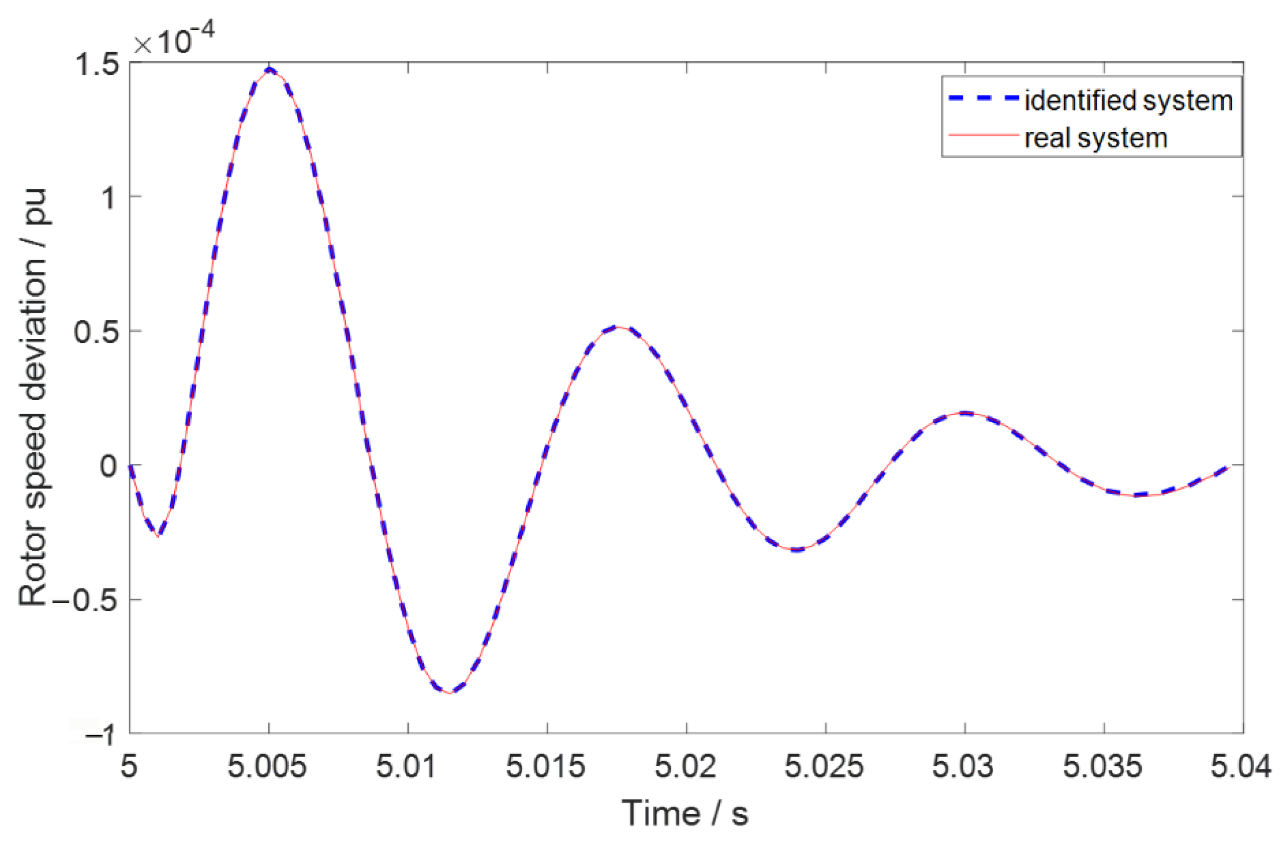
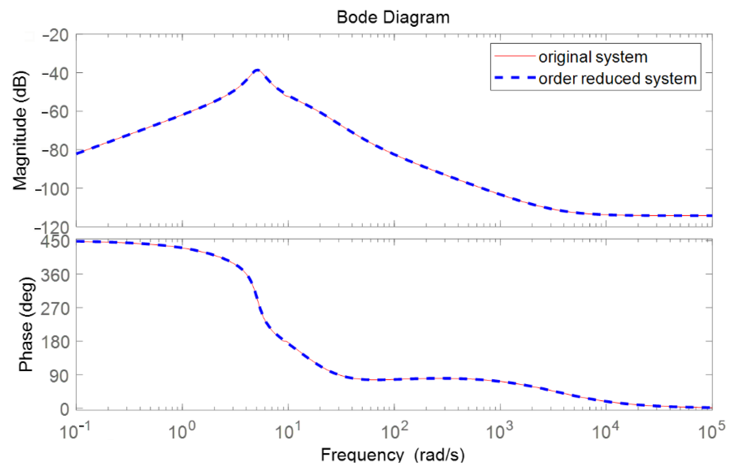
4.1. System Identification

To design the total robust controller of the above system, the rotor speed deviation of the Plant1 Δω₁ is selected as the feedback signal. Furthermore, IPFC 2 is selected as the controller location. By using PRONY identification technology, the system can be obtained.

The identifications are composed of two parts. The first part is the active power supplementary loop identification, which reflects the active power control loop’s damping characteristic. In addition, the second part is the reactive power supplementary loop identification, and it reflects the reactive power control loop’s damping characteristic.

Figure 8 presents the active power control loop identification results and it can be seen that the identified system is basically the same as the real system.

To make controller design more practical, the order of the identified active power loop control system needs to be reduced. In addition, the balanced truncation method is used to reduce the identified system’s order. The Bode diagram comparison of the order reduced system and the original system is given out in Figure 9. Furthermore, the order reduced transfer function is presented in (6).

$$\begin{array}{l}{G}_{\mathrm{P}\_\mathrm{system}}(s)=\frac{-2.594\mathrm{e}-06s^8-0.00225s^7+0.3816s^6}{s^8+22.66s^7+264.4s^6+2995s^5}\\ \frac{+1.354s^5+38.78s^4+146.4s^3+739.1s^2+3128s}{+2.059\mathrm{e}04s^4+1.15\mathrm{e}05s^3+5.784\mathrm{e}05s^2+1.386\mathrm{e}06s+5.328\mathrm{e}06}\end{array}$$

(6)

Similarly, the Bode diagram comparison of the order reduced system and original system of the reactive power control loop is given out in Figure 10 and Figure 11. In addition, the order reduced transfer function is presented in (16).

$$\begin{array}{l}{G}_{\mathrm{Q}\_\mathrm{system}}(s)=\frac{1.932\mathrm{e}-06s^8-0.006458s^7-0.3603s^6}{s^8+31.72s^7+583.9s^6+5914s^5}\\ \frac{-0.4835s^5-4.04s^4+76.62s^3+2235s^2+399.2s}{+5.544\mathrm{e}04s^4+2.836\mathrm{e}05s^3+1.124\mathrm{e}06s^2+3.033\mathrm{e}06s+5.021\mathrm{e}05}\end{array}$$

(7)

4.2. Robust Controller Design

The order of the weight function should not be too high. W₁ is generally a high pass characteristic and W₂ a low pass characteristic. W₃ can be set to a smaller constant. The weight functions selected for different oscillation modes can be different. The weight functions of the robust controller of this paper are given as,

$$\begin{gathered} W_1(s)=\frac{s}{s+100} \\ {W}_2(s)=\frac{100}{s+100} \\ {W}_3(s)=0.5 \end{gathered}$$

After the determination of the weight function, the final controller can be obtained through the Mixed H₂/H_∞ synthesis with regional pole placement. Furthermore, it can be realized through the MATLAT function hinfmix.

$$K_{\mathrm{P}}(s)=\frac{-241.4s^3-3909s^2-1.783\mathrm{e}04s-7265}{s^4+22.18s^3+202.2s^2+883.5s+2124}$$

(8)

$$K_{\mathrm{Q}}(s)=\frac{-56.08s^3+274.3s^2+1.457\mathrm{e}04s+5.051\mathrm{e}04}{s^4+20.72s^3+161.3s^2+686.5s+1180}$$

(9)

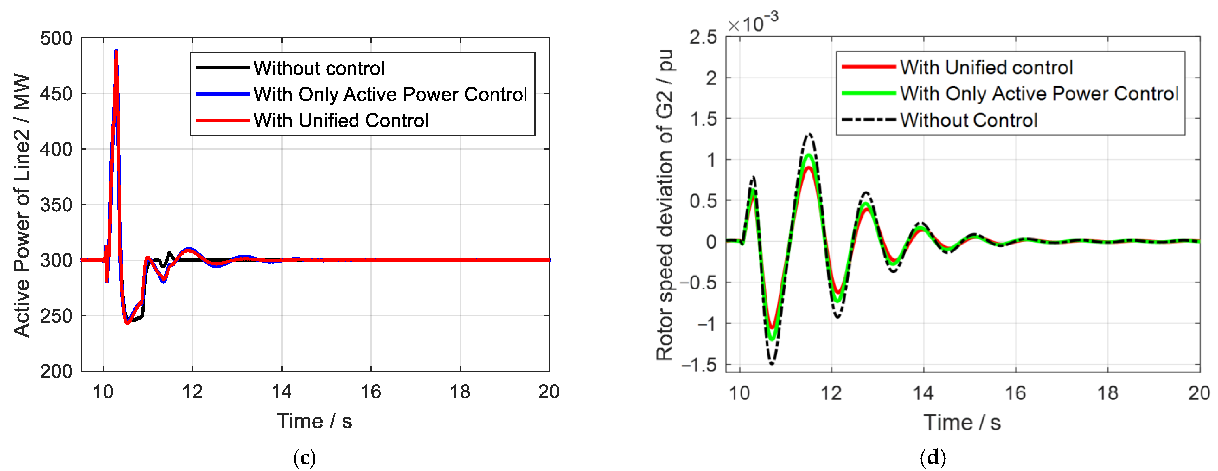
4.3. Case 1 Study: In Single Phase to Ground Fault Situation

The active and reactive power control references of IPFC2 are both set to zero for better comparison, where the damping controller is facilitated. A single phase to ground fault is added at Bus 2 when t = 8 s. Figure 12 gives out the rotor speed deviation of plant 1, active power of plant 1, active power transmitted on Line 2 and the rotor speeds deviation of plant 2 in different control schemes.

It can be seen from Figure 12a that the total control strategy can damp the low-frequency oscillations more effectively. Although the traditional controller with only active power supplementary control can also damp the oscillation, the damping effect is worse than the total control scheme. Figure 12b also presents the output active power of plant 1 with different schemes, which proves the effectiveness of the total control too. Figure 12c shows the active power changing situation in line 2, where the IPFC is located. In addition, it indicates that the supplementary controller can output suitable active power when oscillation occurs, in which case the total controller can output less active power and reaches a better damping effect. Figure 12d also presents the rotor speed deviations of plant2 to demonstrate that the whole system stability can be enhanced with the proposed method. Furthermore,

Table 3. The Damping ratio changing situations with different controls.

Control Strategy	Primary Frequency/Hz	Damping Ratio
Without control	0.81	12%
With only active power control	0.79	24%
With unified power control	1.15	48%

gives the damping ratio changing situations with different controls, it also verifies that the unified power control can enhance the system damping ratio a lot, where the oscillation frequency can be changed because of the control added.

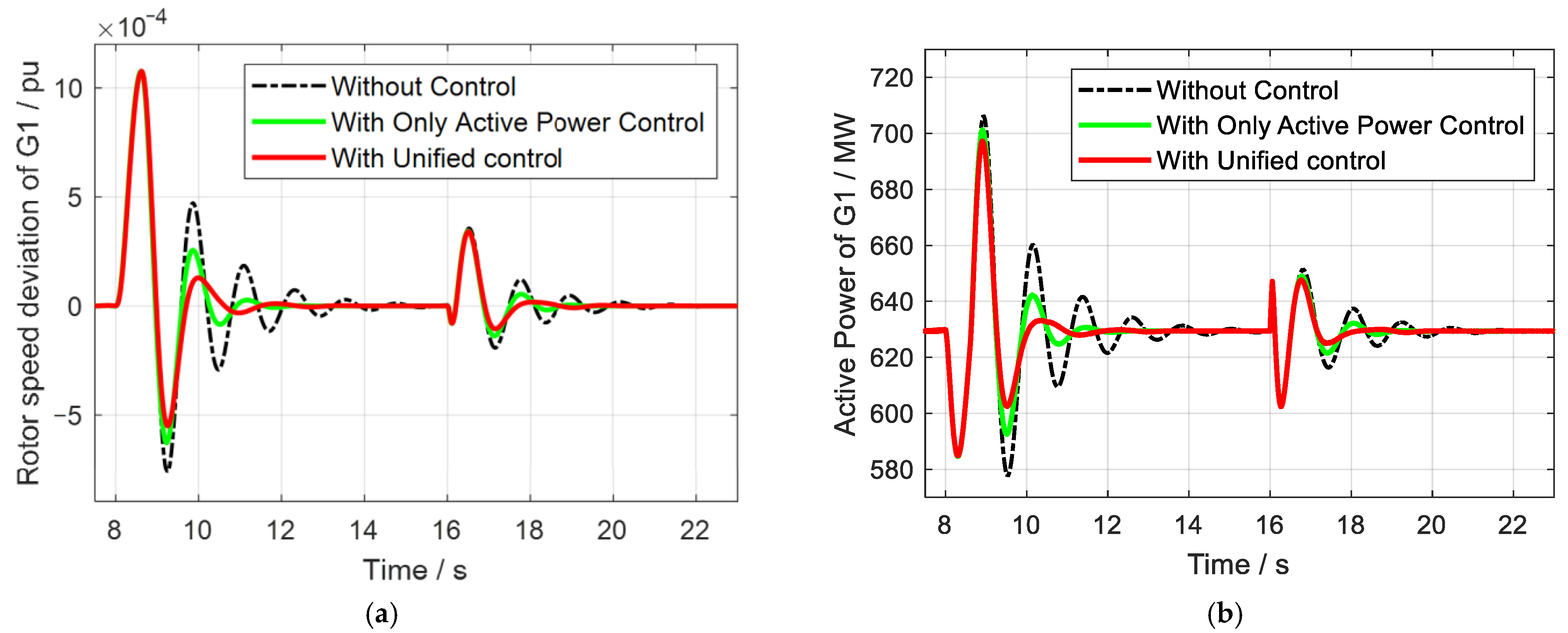
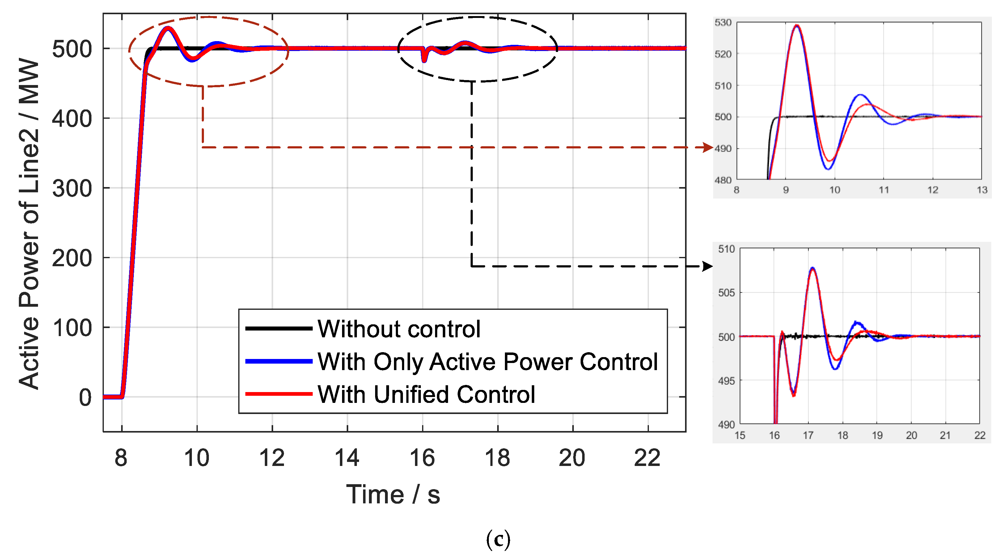
4.4. Case 2 Study: In Temporary Line Disconnection Fault Situation

In this case, A temporary line disconnection fault occurs at line 1 when t = 10 s, and the active power reference of IPFC at line 2 is set as 300 MW such that power transmitted at line 2 is fixed to 300 MW if no supplementary controller is added. Figure 13 gives out the rotor speed deviation of plant 1, active power of plant 1, active power transmitted at line 2, and the rotor speed deviation of plant 2 in different control schemes, respectively. The proposed method can also reach a better damping effect when the fault happens.

Table 4. The Damping ratio changing situations with different controls.

Control Strategy	Primary Frequency/Hz	Damping Ratio
Without control	0.81	12%
With only active power control	0.80	16%
With unified power control	0.79	21%

also gives the damping ratio changing situations with different controls, it also verifies that the effectiveness of the unified power control.

4.5. Case 3 Study: In Cascading Failure Situation

To further prove the robustness and correctness of the proposed method, the cascading failure situation is considered for verification. In this case, the active power reference of IPFC2 is increased from 0 MW to 500 MW at 8 s, and then a 200 Mvar reactive load fluctuation occurs at 16 s. Figure 14 gives out the rotor speed deviation of plant 1, active power of plant 1, and active power transmitted at line 2 in different control schemes, respectively. According to the results in these figures, the proposed total damping control strategy can be demonstrated as correct and robust. In addition,

Table 5. The Damping ratio changing situations with different controls.

Control Strategy	Primary Frequency/Hz	Damping Ratio
Without control	0.83	12%
With only active power control	0.67	36%
With unified power control	0.59	41%

gives the damping ratio changing situations as additional verification.

5. Conclusions

According to the study, it can be concluded that:

• The IPFC can be used for LFO damping and can reach satisfying effect. Especially, the different active and reactive outer current control loops can be used for oscillation control. Furthermore, the control can still be effective even one controller is out of operation.
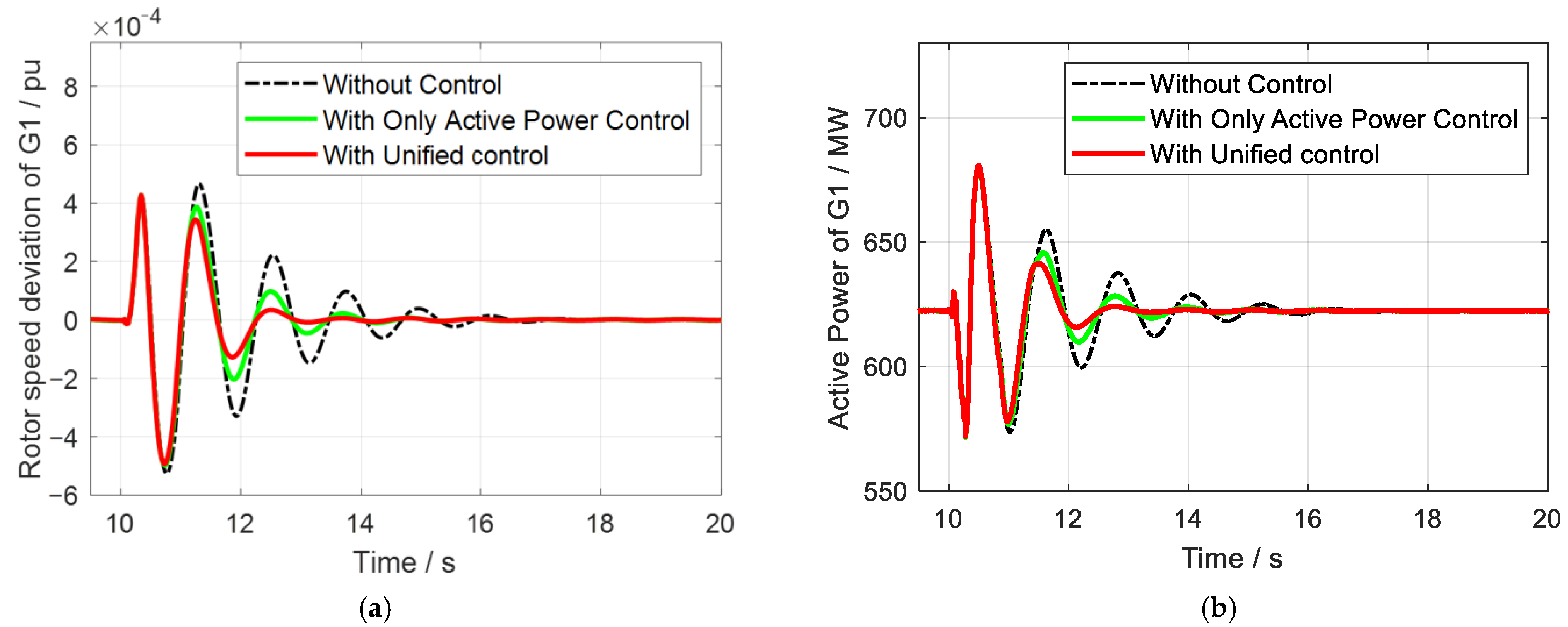
• Compared with only one active outer control loop situation, the total control scheme with a reactive controller has more advantages. With such a design, a better control effect can be obtained, and almost 50% ratio increment can be reached with unified control compared with only active power control.
• The robust controller design through LMI and PRONY method is effective to suppress the low-frequency oscillations. In addition, the LFO can both be quickly eliminated whether it is in fault, power disturbance, and operation vary occasions. Furthermore, the damping ratio of the controlled system can increase to 48%, 21%, and 41%, respectively.

References

1. Li, R.; Wong, P.; Wang, K.; Li, B.; Yuan, F. Power quality enhancement and engineering application with high permeability distributed photovoltaic access to low-voltage distribution networks in Australia. Prot. Control Mod. Power Syst. 2020, 5, 18. [Google Scholar] [CrossRef]
2. Shang, L.; Guo, H.; Zhu, W. An improved MPPT control strategy based on incremental conductance algorithm. Prot. Control Mod. Power Syst. 2020, 5, 14. [Google Scholar] [CrossRef]
3. Jiang, Q.; Zeng, X.; Li, B.; Wang, S.; Liu, T.; Chen, Z.; Wang, T.; Zhang, M. Time-Sharing Frequency Coordinated Control Strategy for PMSG-Based Wind Turbine. IEEE J. Emerg. Sel. Top. Circuits Syst. 2022, 12, 268–278. [Google Scholar] [CrossRef]
4. Liu, Y.; Meliopoulos, A.P.; Sun, L.; Choi, S. Protection and control of microgrids using dynamic state estimation. Prot. Control Mod. Power Syst. 2018, 3, 31. [Google Scholar] [CrossRef] [Green Version]
5. Tao, Y.; Li, B.; Dragicevic, T.; Liu, T.; Blaabjerg, F. HVDC Grid Fault Current Limiting Method Through Topology Optimization Based on Genetic Algorithm. IEEE J. Emerg. Sel. Top. Power Electron. 2020, 9, 7045–7055. [Google Scholar] [CrossRef]
6. Tao, Y.; Li, B.; Liu, T. Pole-to-ground fault current estimation in symmetrical monopole high-voltage direct current grid considering modular multilevel converter control. Electron. Lett. 2020, 56, 392–395. [Google Scholar] [CrossRef]
7. Jiang, Q.; Li, B.; Liu, T.; Wang, P. Fault current limiting method based on virtual impedance for hybrid high-voltage direct current with cascaded MMC inverters. Electron. Lett. 2021, 57, 229–231. [Google Scholar] [CrossRef]
8. Gandoman, F.H.; Ahmadi, A.; Sharaf, A.M.; Siano, P.; Pou, J.; Hredzak, B.; Agelidis, V.G. Review of FACTS technologies and applications for power quality in smart grids with renewable energy systems. Renew. Sustain. Energy Rev. 2018, 82, 502–514. [Google Scholar] [CrossRef]
9. Singh, B.; Kumar, R. A comprehensive survey on enhancement of system performances by using different types of FACTS con-trollers in power systems with static and realistic load models. Energy Rep. 2020, 6, 55–79. [Google Scholar] [CrossRef]
10. Taher, M.A.; Kamel, S.; Jurado, F.; Ebeed, M. Optimal power flow solution incorporating a simplified UPFC model using lightning attachment procedure optimization. Int. Trans. Electr. Energy Syst. 2020, 30, e12170. [Google Scholar] [CrossRef]
11. Lei, Y.; Li, T.; Tang, Q.; Wang, Y.; Yuan, C.; Yang, X.; Liu, Y. Comparison of UPFC, SVC and STATCOM in Improving Commutation Failure Immunity of LCC-HVDC Systems. IEEE Access 2020, 8, 135298–135307. [Google Scholar] [CrossRef]
12. Wahhade, S.N.; Gowder, C. Enhancement of power flow capability in power system using UPFC-a review. Int. Res. J. Eng. Technol. 2019, 6, 1146–1150. [Google Scholar]
13. Singh, P.; Senroy, N. Steady-state model of VSC based FACTS devices using flexible holomorphic embedding: (SSSC and IPFC). Int. J. Electr. Power Energy Syst. 2021, 133, 107256. [Google Scholar] [CrossRef]
14. Kalyan, C.H.; Rao, G.S. Impact of communication time delays on combined LFC and AVR of a multi-area hybrid system with IPFC-RFBs coordinated control strategy. Prot. Control Mod. Power Syst. 2021, 6, 7. [Google Scholar] [CrossRef]
15. Jiang, Q.; Li, B.; Liu, T. Investigation of hydro-governor parameters’ impact on ULFO. IET Renew. Power Gener. 2019, 13, 3133–3141. [Google Scholar] [CrossRef]
16. Wang, P.; Li, B.; Jiang, Q.; Chen, G.; Han, X.; Dragicevic, T.; Liu, T. The occurrence mechanism and damping method of ultra-low-frequency oscillations. IET Renew. Power Gener. 2021, 15, 1100–1115. [Google Scholar] [CrossRef]
17. Jiang, S.; Gole, A.M.; Annakkage, U.D.; Jacobson, D.A. Damping Performance Analysis of IPFC and UPFC Controllers Using Validated Small-Signal Models. IEEE Trans. Power Deliv. 2010, 26, 446–454. [Google Scholar] [CrossRef]
18. Mishra, S.; Dash, P.; Hota, P.; Tripathy, M. Genetically optimized neuro-fuzzy IPFC for damping modal oscillations of power system. IEEE Trans. Power Syst. 2002, 17, 1140–1147. [Google Scholar] [CrossRef]
19. Parimi, A.M.; Elamvazuthi, I.; Kumar, A.V.P.; Cherian, V. Fuzzy logic based control for IPFC for damping low frequency oscillations in multimachine power system. In Proceedings of the 2015 IEEE IAS Joint Industrial and Commercial Power Systems/Petroleum and Chemical Industry Conference (ICPSPCIC), Hyderabad, India, 19–21 November 2015; pp. 32–36. [Google Scholar] [CrossRef]
20. Almunif, A.; Fan, L.; Miao, Z. A tutorial on data-driven eigenvalue identification: Prony analysis, matrix pencil, and eigensystem realization algorithm. Int. Trans. Electr. Energy Syst. 2020, 30, e12283. [Google Scholar] [CrossRef] [Green Version]
21. Isbeih, Y.J.; El Moursi, M.S.; Xiao, W.; El-Saadany, E. H mixed-sensitivity robust control design for damping low-frequency oscillations with DFIG wind power generation. IET Gener. Transm. Distrib. 2019, 13, 4274–4286. [Google Scholar] [CrossRef]
Figure 1. The structure of IPFC.
Processes 10 02064 g001
Figure 2. The control strategies of mainly controlled converter in IPFC.
Processes 10 02064 g002
Figure 3. The control strategies of auxiliary-controlled converter in IPFC.
Processes 10 02064 g003
Figure 4. The control diagrams of Total Supplementary Damping control for IPFC.
Processes 10 02064 g004
Figure 5. The relationship between the supplementary control and system.
Processes 10 02064 g005
Figure 6. The total robust LFO suppress strategy for IPFC.
Processes 10 02064 g006
Figure 7. The test system with IPFC.
Processes 10 02064 g007
Figure 8. The identified curve of active power control loop.
Processes 10 02064 g008
Figure 9. Bode diagram comparison of the order reduced system and original system of active power control loop.
Processes 10 02064 g009
Figure 10. The comparison between the real curve and identified curve of reactive power control loop.
Processes 10 02064 g010
Figure 11. Bode diagram comparison of the order reduced system and original system of active power control loop.
Processes 10 02064 g011
Figure 12. Simulation situations in case1. (a) The rotor speeds deviation of plant 1 with and without control in different situations. (b) The output active power of plant 1 with and without control in different situations. (c) The active power transmitted on Line 2 with and without control in different situations. (d) The rotor speeds deviation of plant 2 with and without control in different situations.
Processes 10 02064 g012
Figure 13. Simulation situations in case2. (a) The rotor speeds deviation of plant 1 with and without control in different situations. (b) The output active power of plant 1 with and without control in different situations. (c) The active power transmitted on Line 2 with and without control in different situations. (d) The rotor speeds deviation of plant 2 with and without control in different situations.
Processes 10 02064 g013aProcesses 10 02064 g013b
Figure 14. Simulation situations in case3. (a) The rotor speeds deviation of plant 1 with and without control in different situations. (b) The output active power of plant 1 with and without control in different situations. (c) The active power transmitted on Line 2 with and without control in different situations.
Processes 10 02064 g014aProcesses 10 02064 g014b