Article

Nonstationary Process Monitoring Based on Alternating Conditional Expectation and Cointegration Analysis

College of Chemical Engineering, Beijing University of Chemical Technology, Beijing 100029, China
*
Authors to whom correspondence should be addressed.
Processes 2022, 10(10), 2003; https://doi.org/10.3390/pr10102003
Submission received: 31 August 2022 / Revised: 23 September 2022 / Accepted: 26 September 2022 / Published: 4 October 2022
(This article belongs to the Section Process Control and Monitoring)

Abstract

:
Traditional multivariate statistical methods, which are often used to monitor stationary processes, are not applicable to nonstationary processes. Cointegration analysis (CA) is considered an effective method to deal with nonstationary variables. If there is a cointegration relationship among the nonstationary series in the system, it indicates that a stable long-term dynamic equilibrium relationship exists among these variables. However, due to the complexity of modern industrial processes, there are nonlinear relations between variables, which are not considered by the traditional linear cointegration theory. Alternating conditional expectation (ACE) can perform nonlinear transformation on these variables to maximize the linear correlation of the transformed variables. It will be helpful to deal with the nonlinear relations by modeling with transformed variables. In this work, a new monitoring strategy based on ACE and CA is proposed. The data are first transformed by an ACE algorithm, CA is performed after that, and then monitoring statistics are calculated to determine whether the system is faulty. The strategy is applied to the monitoring of a simulation case and a catalytic reforming unit in a petrochemical company. The results show that the strategy can realize the monitoring of nonstationary process, with a higher fault detection rate and a lower false alarm rate compared with the monitoring strategy based on traditional cointegration theory.

1. Introduction

With the increasing scale and complexity of the modern production industry, the probability of system fault also increases, which may cause economic losses or even major safety incidents. Therefore, it is particularly necessary to monitor the production process. Due to the wide application of distributed control system (DCS), a large number of industrial process data have been recorded [1,2], and data-driven process monitoring methods have developed rapidly with the application of computer technology and artificial intelligence technology in process monitoring. The characteristics of historical data can be extracted by data-driven monitoring methods without detailed modeling of the internal mechanism of the process.
As a traditional data-driven method, multivariate statistical process monitoring (MSPM) has been widely used in the monitoring of stationary processes. The high-dimensional samples are projected into the low-dimensional subspace through MSPM, and the monitoring statistics in the low-dimensional subspace are calculated to monitor the process operation status [3].
Among the methods based on multivariate statistics, principal components analysis (PCA) is one of the classical algorithms. The covariance matrix of the process data set is calculated to obtain the eigenvector of the matrix, so as to determine the direction of the reduced dimension projection [4]. Partial least squares (PLS) is similar to PCA. The basic idea of PLS is to establish a small number of input and output comprehensive variables, so as to reflect the change information contained in the original variables more intensively, and then a linear regression model is established [5]. The square prediction error (SPE) and Hotelling’s statistics ( T 2 ) are calculated to achieve process monitoring in these two methods [6]. However, it is usually assumed in traditional MSPM that the relationship among process variables is linear and variables are stationary. Dynamic and nonstationary characteristics in the process are not taken into account, which refers to the autocorrelation and time-varying characteristics of variables. The abnormal deviations at an early stage of process faults could be buried in these nonstationary trends, and cannot be effectively detected in time [7]. Therefore, several new monitoring methods are proposed for the complex characteristics of the process.
In order to deal with the dynamic characteristics of the process, Ku proposed dynamic principal components analysis (DPCA) on the basis of PCA [8]. The time-lagged variables of the original data were extended to reflect the dynamic relationship among variables. However, Rato [9] pointed out that the principal components extracted by DPCA still retain strong autocorrelation, which result in reduced monitoring performance of T 2 and SPE. A common way to deal with the nonstationary process is to make several differences on the nonstationary variables to obtain the stationary variables and then establish the monitoring model. The autoregressive integrated moving average model (ARIMA) was first proposed by Box and Jenkins [10], whose basic idea is to analyze the characteristics of autocorrelation and partial autocorrelation functions of stationary series after difference, and the parameters of the model are calculated to test the effectiveness of the model to predict the future time series. However, the dynamic information of the process is lost after the difference, which makes the monitoring model less effective.
Cointegration analysis (CA) was first proposed by Engle to deal with nonstationary economic variables [11]. Hendry proposed the error correction model (ECM) in 1978, through which the nonstationary series are converted into stationary series without difference modeling. Granger proposed the relationship between cointegration and ECM in 1981 [12]. In 1987, Engle and Granger integrated the vector autoregressive model (VAR), ECM and cointegration theory to form the Granger representation theorem. Through this theory, the advantages of short-term and long-term models in time series analysis are combined, which provides a better solution for the modeling of nonstationary time series. Due to the internal physical and chemical mechanism of modern industrial process, there is a long-term dynamic equilibrium relationship among variables, which can be handled by cointegration theory. Therefore, CA has been widely used in the industrial field in recent years. Chen applied CA to the industrial field for the first time and introduced the reduced-order model diagnosis method to isolate the system fault. The simulation example in the fluid catalytic cracking unit (FCCU) system showed that cointegration has a good prospect in the application of condition monitoring and fault diagnosis for engineering systems [13].
Xu revealed the shortcomings of the monitoring strategy based on the traditional unit root test method which is insensitive to some system faults and the limitations of the reduced order cointegration model method through some examples, and put forward the method of using the unit root of structural mutation and the Gregory–Hansen cointegration test to carry out system condition monitoring and fault diagnosis. The results showed that the deficiencies of the ADF test were remedied and the variables containing fault information can be directly determined [14]. Yu proposed an adaptive monitoring scheme based on recursive CA to address the issues that when the cointegration relationship changes, the operation status of future nonstationary process could not be reflected accurately by the previous CA. Three monitoring statistics were developed to reflect the operation status of the industrial process, and experimental results of two real industrial processes showed that the adaptive monitoring strategy based on recursive CA could effectively adapt to normal process changes without frequent model updating [15]. A new monitoring index that contains multiple order moments was proposed by Wen [16] to capture different statistical features of the stationary data set. The results showed that the use of multiple order moments as a monitoring index based on cointegration analysis can provide early alarms for abnormal conditions and can effectively identify normal changes and abnormalities.
In simple terms, if a linear combination of a group of nonstationary time series is stationary, it means that linear cointegration exists in the time series. However, the traditional linear cointegration model is not sensitive enough to some faults when the relationship of most industrial process variables is nonlinear, which should be considered when establishing the monitoring model.
Alternating conditional expectation (ACE) was proposed by Breiman [17] and improved by Xue [18] through replacing the conditional expectation calculation of finite data sets with a data smoothing technique called Supermoore. The basic principle of ACE is to transform the dependent variable and the independent variable to maximize the linear correlation between the transformed dependent variable and the independent variable.
Zhang [19] applied it to answer the question that if the sequences Y t and X t are nonstationary and non-cointegrated, then under what conditions the cointegration relationship exists between the nonlinear transformation f ( Y t ) and g ( X t ) . He pointed out that it is not necessary to consider whether there is a cointegration relationship between the transformed sequence f ( Y t ) and g ( X t ) any more if there is a cointegration relationship identified between Y t and X t . In such a case, the theory of linear cointegration can perform well. On the contrary, if there is no cointegration relationship between Y t and X t , the existing linear cointegration theory will no longer be applicable. In this case, the establishment of the structural model of the transformed sequence f ( Y t ) and g ( X t ) will broaden the application scope of the cointegration theory.
Based on above discussion, a new monitoring strategy is proposed in this paper. An ACE algorithm is used to transform historical data to maximize the linear correlation between variables, then CA is used to analyze the cointegration relationship among variables and establish the cointegration model, and finally the statistics are calculated to monitor the process. The strategy is applied to the monitoring of a simulation case and a catalytic reforming unit in a petrochemical company. The results show that this method can realize the monitoring of nonstationary process and find the equilibrium relationship which cannot be found by the traditional cointegration method, and it can improve the sensitivity of the monitoring model.
The rest of this paper is organized as follows: the theories and methods used in this paper are introduced in Section 2. The detailed steps of the method proposed in this paper are introduced in Section 3. Three cases are used to verify the effectiveness of the proposed method in Section 4, including two simulation cases and a real industrial case. Finally, the paper is concluded in Section 5.

2. Theory and Method

2.1. Difference and Unit Root Test

If a nonstationary series becomes stationary by differencing it d times, it is called integrated of order d , which can be also represented as: X ~ I ( d ) . When d = 1 , the difference process is called unit root process. In this paper, we only discuss the case of d = 1 as most nonstationary signals can be considered as the 1st order cointegration, if linear cointegration exists. A unit root test can be used to determine whether a time series is consistent with a unit root process.
A popular tool to test whether a time series is stationary is Augmented Dickey–Fuller (ADF) [20]. An autoregressive model can be written as the following form:
y t = a 1 y t 1 + a 2 y t 2 + + a p y t p + u t ,
where p is the lag order, u t   is the random part of a sequence. The characteristic Equation of the above formula is:
λ p a 1 λ p 1 a p = 0 ,
If the obtained p nonzero eigenvalues λ 1 , λ 2 , , λ p are all within the unit circle, the sequence y t is stationary. Otherwise, there is at least one unit root, assuming λ 1 = 1 , Equation (2) can be written as:
1 a 1 a 2 a p = 0 ,
This shows that if the series is nonstationary, the sum of the regression coefficients is 1. Equation (1) can be transformed into:
y t = ρ y t 1 + i = 1 p 1 θ i Δ y t i + u t ,
in which: ρ = j = 1 p α j , θ i = j = i + 1 p α j , ( i = 1 , 2 , , p 1 ) . When ρ < 0 , the series is stationary.
Parameters in Equation (4) are estimated by ordinary least squares and ρ is tested to determine whether the series is stationary.

2.2. Cointegration Theory

The basic idea of cointegration theory is that although a set of variables are nonstationary over time, they will change together and maintain a common long-term random trend. The random trend can be eliminated by linear combination, and a stationary series can be obtained. It can be considered that there is a long-term equilibrium relationship between them.
On the concept of simple integration, the cointegration theory can be further explained. x 1 t , x 2 t , x 3 t x i t are nonstationary series, where x i t ~ I ( 1 ) ,   i = 1 , 2 , 3 i . These series meet the cointegration relationship if the following equation can be established by a set of coefficients,   α 1 , α 2 , α 3 α i :
ξ = α 1 x 1 t + α 2 x 2 t + α 3 x 3 t + + α i x i t ,
where ξ is a stationary series of I ( 0 ) , and α i is called the cointegration coefficient. The equation above can be explained as follows: the linear combination of a group of I ( 1 )   variables can derive an I ( 0 ) variable, then these variables are cointegrated.

2.3. Cointegration Test

2.3.1. Engle and Granger Test

In order to test whether there is a cointegration relationship between two sequences Y t and X t , Engle and Granger proposed a two-step test, also known as the EG test, in 1987.
Step 1: estimate the following equation with ordinary least squares regression:
Y t = c + β X t + μ t ,
in which c is the constant term, β is the regression coefficient, and μ t is the residual sequence, which can be calculated as follows:
μ ^ t = Y t Y ^ t = Y t α ^ β ^ X t ,
Step 2: carry out the ADF test mentioned above on μ ^ t , if the residual sequence is stationary, Y t and X t are cointegrated.
The EG test is mainly applicable to the cointegration test between two variables, and not applicable when there are multiple cointegration relationships between variables.

2.3.2. Johansen Test

The Johansen test [21,22] based on the VAR model is a method which is used to determine the cointegrated relationship among multiple nonstationary variables. The VAR model can be described as follows:
Y t = j = 1 p A j Y t j + D t + U t ,
where Y t R m   is a m-dimensional series, A j R m × m is the coefficient matrix, and U t is an m-dimensional white noise that conforms to normal distribution.
The vector error-correction (VEC) model transformed from Equation (8) can be expressed as:
Δ Y t = Π Y t 1 + j = 1 p 1 A j * Δ Y t j + D t + U t ,
Π = A ( 1 ) = I j = 1 p A j ,
A j * = i = j + 1 p A i , j = 1 , 2 , , p 1 ,
Π can be estimated by the maximum likelihood estimate (MLE). Depending on its rank, if rank ( Π ) = 0: there is no cointegrated relationship between the series. The number of cointegrated relationship can be calculated by testing the significance of the characteristic roots of Π . The characteristic roots of Π are sorted in descending order, λ 1 > λ 2 > > λ m . If there are r cointegrated vectors, the other characteristic roots should be zero. The number of cointegration relationships can be obtained by a trace test of characteristic roots, of which statistics can be calculated by:
λ t r a c e ( r ) = T i = r + 1 m ln ( 1 λ i ^ ) ,
The critical value of the statistic can be obtained by the Monte Carlo method, then the number of independent cointegration vectors can be determined. Π is decomposed into two full rank matrices:
Π = Γ B ,
where   Γ , B ϵ R m × r , 0 < r < m , then:
ξ t = B x t ,
in which ξ t is a stationary series, and B is the cointegration coefficient matrix.

2.4. Alternating Conditional Expectation

A method is provided by the ACE algorithm to derive a pair of nonlinear transformation functions f ( · ) and g ( · ) to maximize the correlation between f ( Y t ) and g ( X t ) . If f ( Y t ) is regressed to g ( X t ) to calculate goodness of fit R 2 , the ACE algorithm is equivalent to selecting nonlinear transformation function to maximize goodness of fit R 2 , which makes Equation (15) a significant regression relation expression.
f ( Y t ) = g ( X t ) + μ t ,
where μ t is the random errors. f ( · ) and g ( · ) are used to minimize the sum of squares of residuals in the above regression relationship, that is:
( f , g ) = a r g   min f , g t T [ f ( Y t ) g ( X t ) ] 2 ,
The process of finding the optimal transformation function by the ACE algorithm is an iterative process. The mean square error of the simple linear regression process is defined:
e 2 ( f , g ) = E [ f ( Y t ) g ( X t ) ] 2 ,
the e 2 ( f , g ) for f ( Y t ) are minimized and if E [ f 2 ] = 1 , the result is:
f 1 ( Y ) = E [ g ( X t ) | Y t ] | | E [ g ( X t ) | Y t | | ,  
where | | · | | = [ E ( · ) 2 ] 1 / 2 , then the next step of ACE algorithm is minimizing the e 2 ( f 1 , g ) for g ( X t ) . The result is:
g 1 ( X t ) = E [ f 1 ( Y t ) | X t ] ,
The process to calculate nonlinear transformation functions ( f 1 ( · ) , g 1 ( · ) ) is the first iteration in the whole ACE calculation. The iterative process will continue until the value of e 2 ( f , g ) is no longer reduced. The iterative basis is defined as follows:
f m ( Y t ) = E [ g m 1 ( X t ) | f m 1 ( Y t ) ]   | | E [ g m 1 ( X t ) | f m 1 ( Y t ) | | ,  
g m ( X t ) = E [ f m ( Y t ) | g m 1 ( X t ) ]   ,
where the initial values are f 0 ( Y t ) = Y t / | | Y t | | , g 0 ( X t ) = X t .

2.5. Monitoring Statistics

A stationary multivariate series can be combined by cointegration test:
ξ t = β ^ x t + μ ^ ,
where ξ t is a stationary multivariate series, so it can be monitored by traditional multivariate statistical methods. When the process becomes abnormal, the long-term equilibrium relationship among variables will be broken, and the statistical characteristics of ξ t will also change.
The monitoring of process operation status can be realized through monitoring the statistical characteristics of ξ t . The original nonstationary variables are projected into a new space through the cointegration vector, and the common random trend among variables is eliminated. The stochastic trends in residual subspace can be extracted as:
τ t = β T x t ,
τ t is differenced to eliminate its nonstationary trend.
Δ τ t = β T ( x t x t 1 ) ,
T τ 2 statistic is constructed as:
T τ 2 = Δ τ T Λ z 1 Δ τ ,
T τ 2   is used to monitor the change of nonstationary part [23], which is similar to T 2 statistic in PCA. The control limit C can be obtained by kernel density estimation.

3. The Proposed Monitoring Strategy

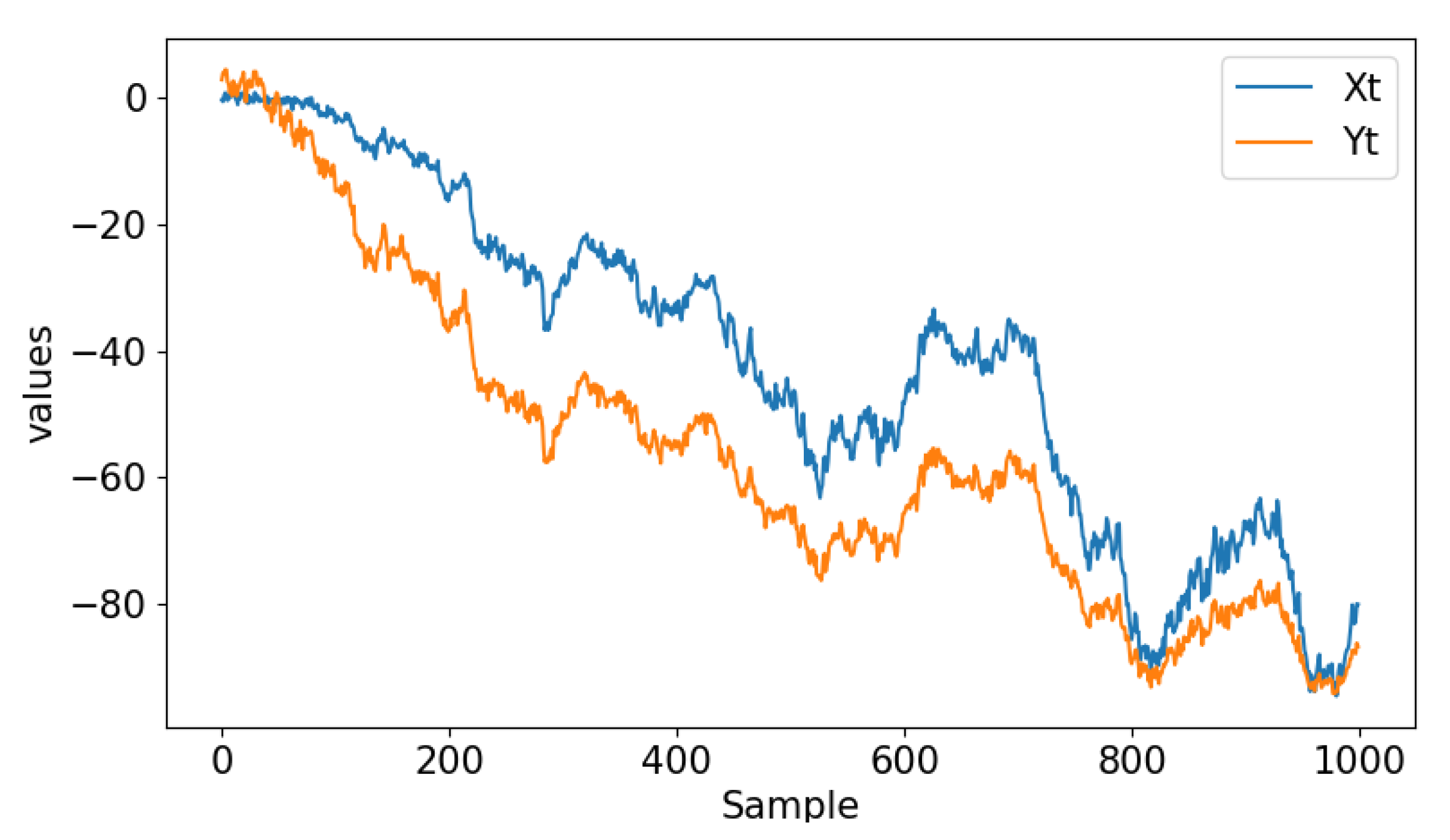
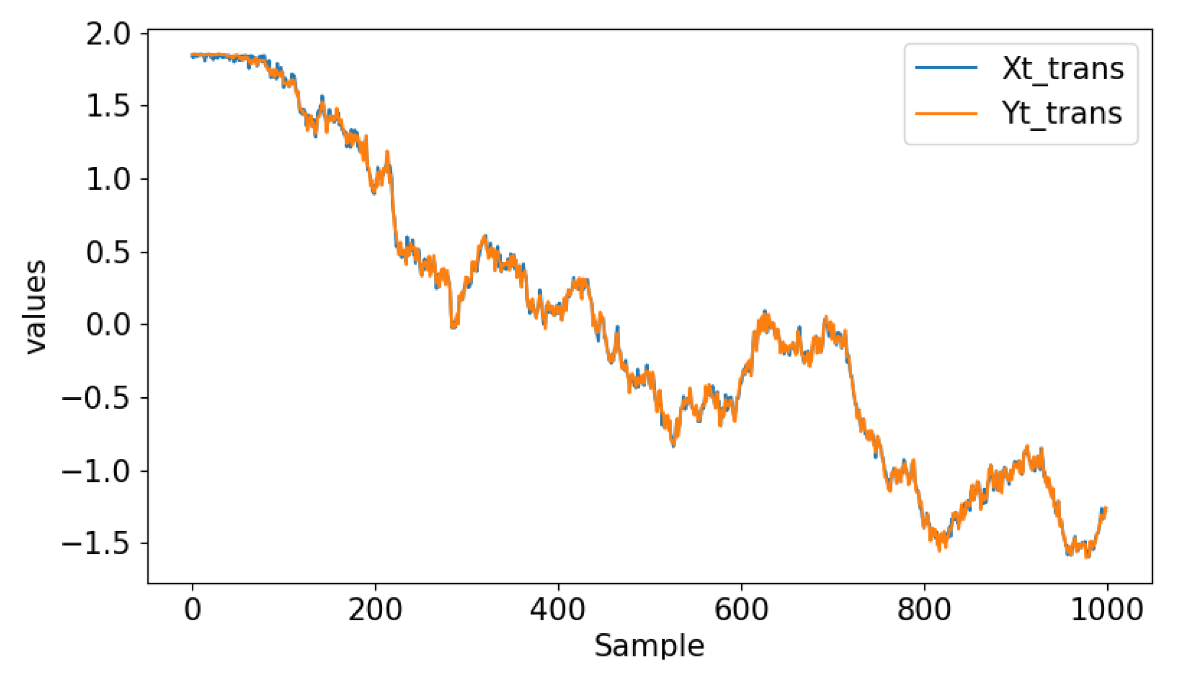
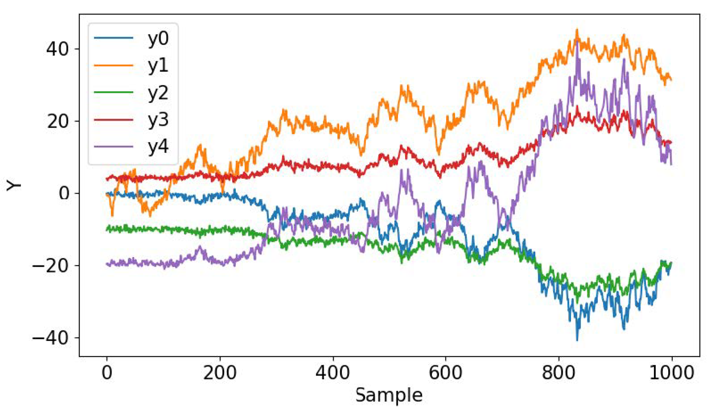
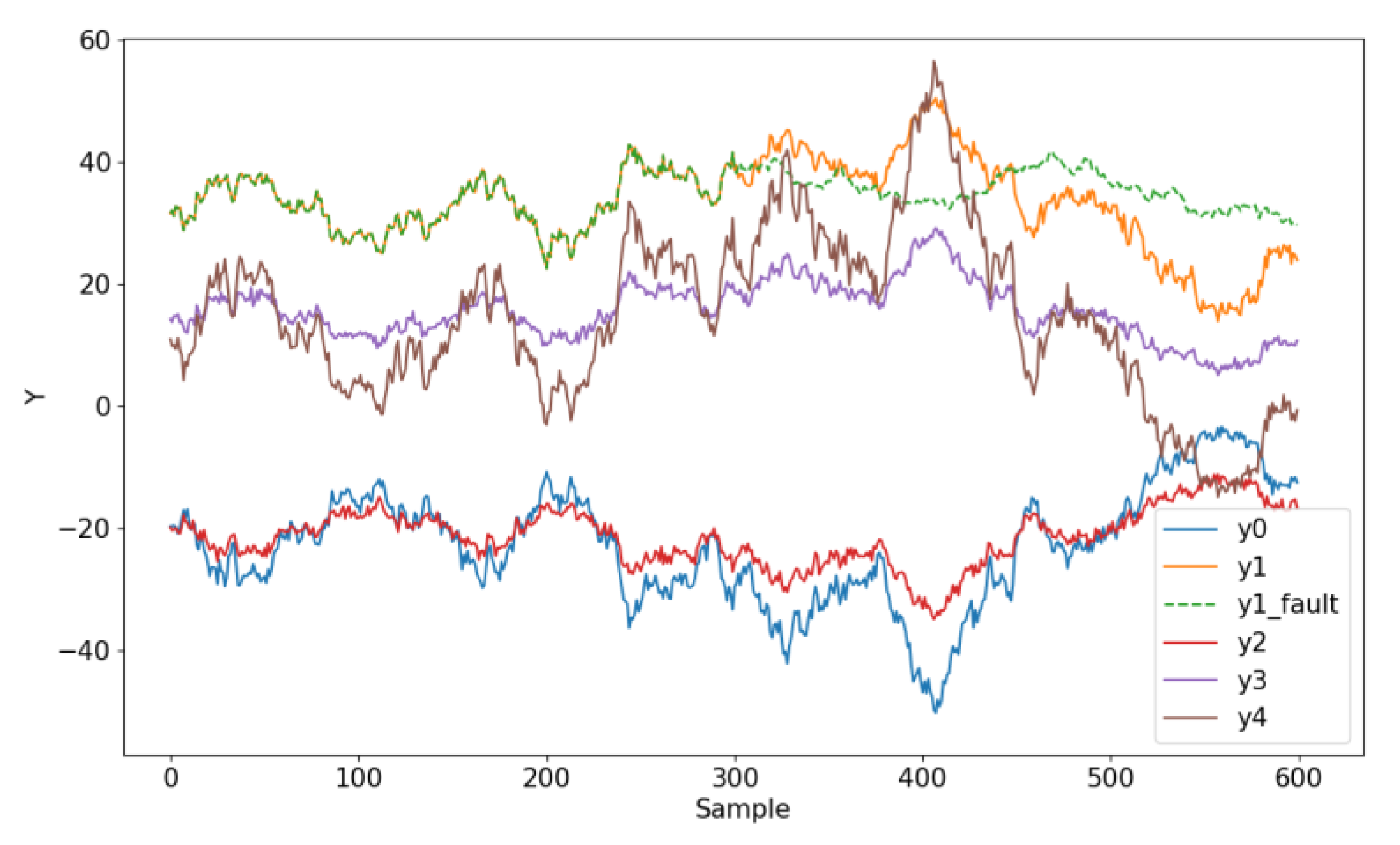
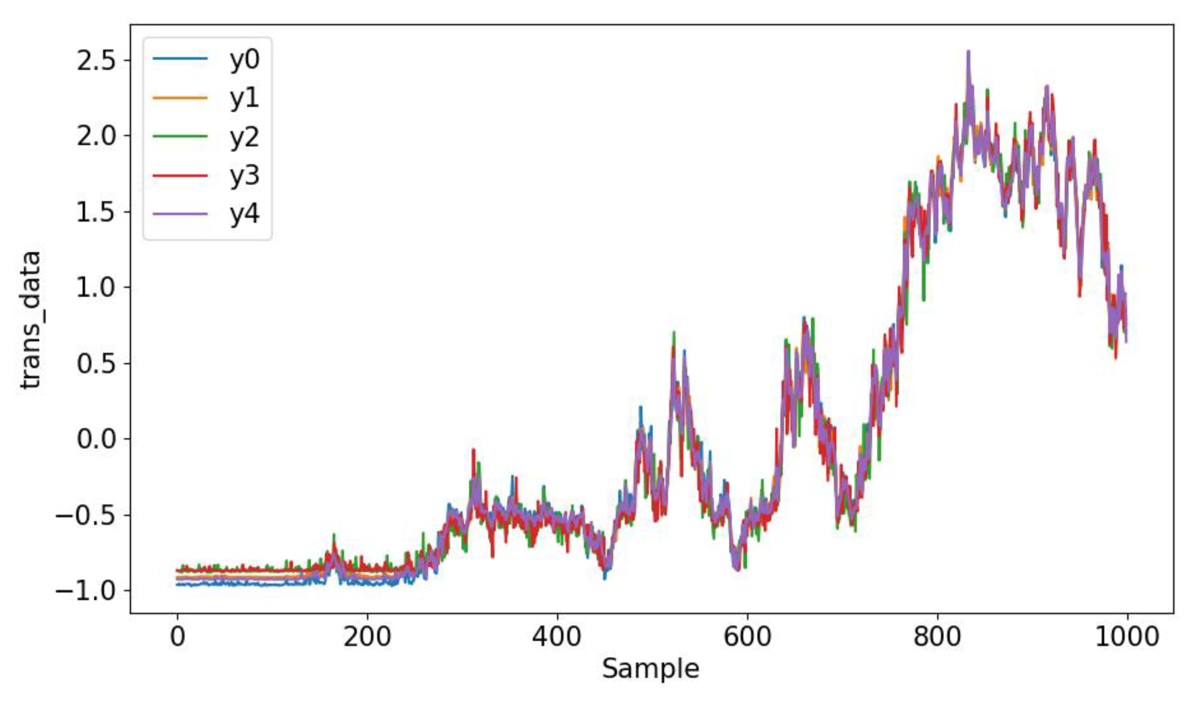
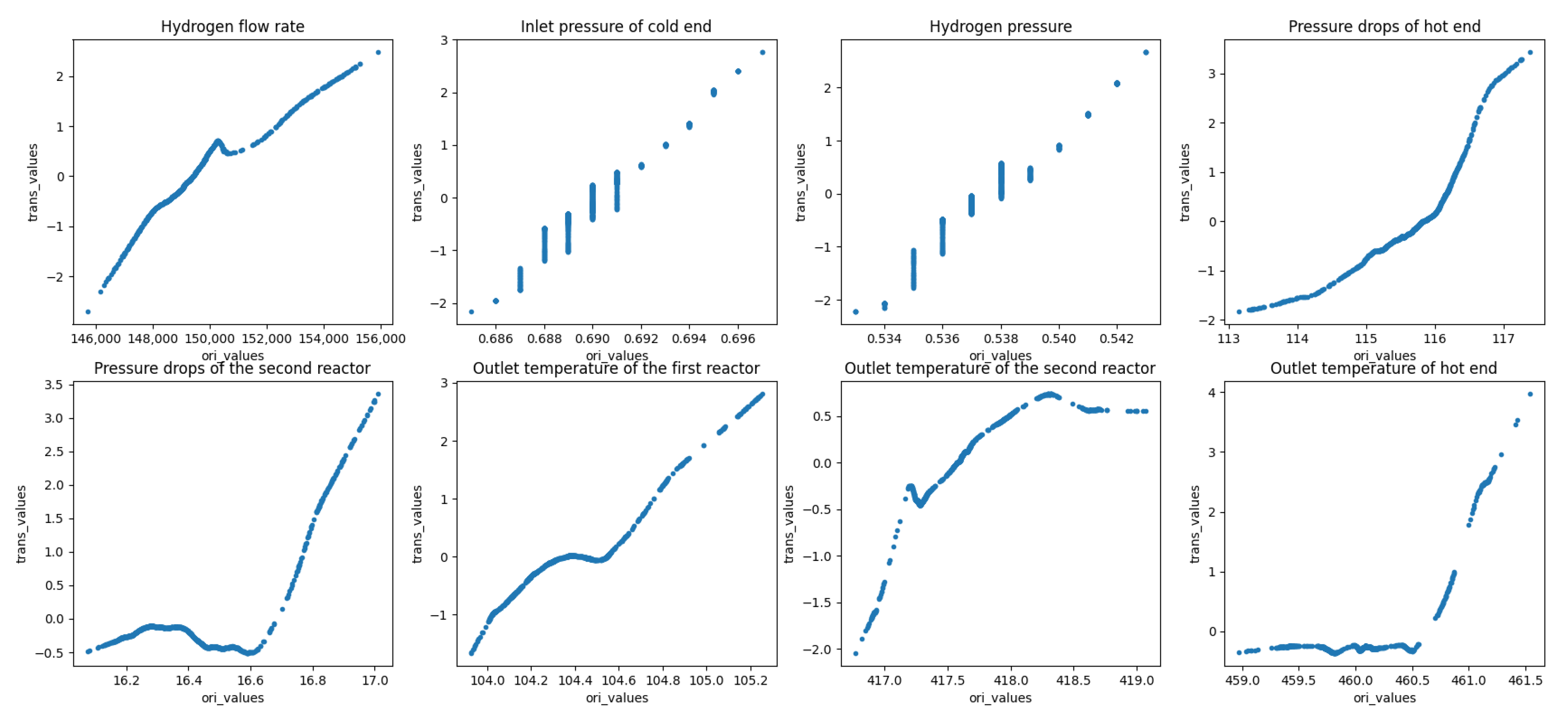
Nonstationary working conditions often exist in actual industrial production. The nonstationary trend of variables cannot be distinguished from the trend caused by an abnormal process through the traditional multivariate statistical method. The change of a long-term equilibrium relationship among nonstationary variables can be monitored instead of the nonstationary variables themselves by CA. However, the traditional linear cointegration model is not sensitive to some faults if there is a nonlinear relationship among certain process variables. The purpose of the ACE algorithm is to find a pair of nonlinear transformation functions that maximize the linear correlation of the transformed sequences. Therefore, establishing the structural model of the transformed sequence will broaden the application range of the cointegration theory.
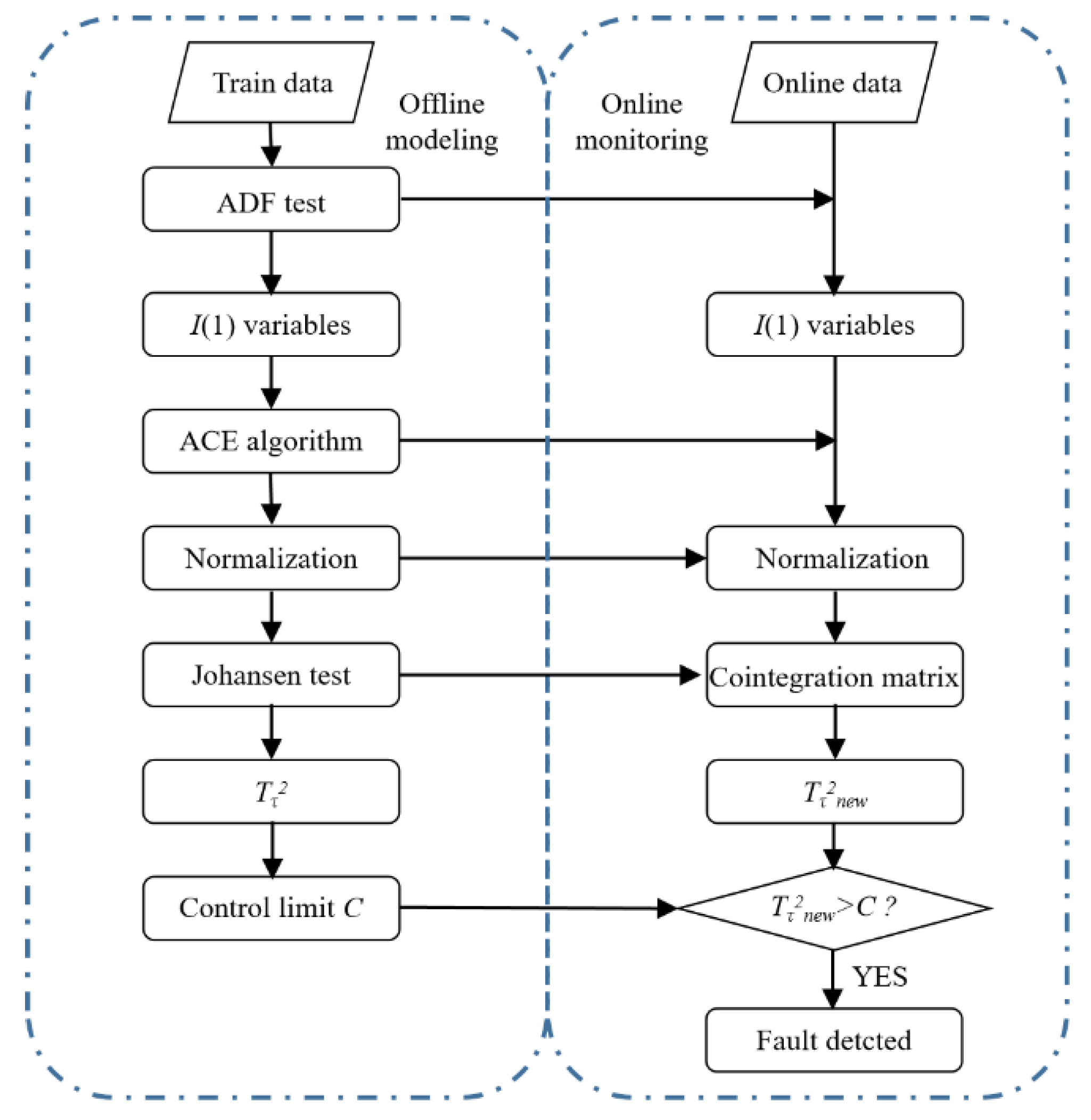
The monitoring strategy based on ACE and CA is proposed in this article. The algorithm block diagram is as shown in Figure 1.

3.1. Offline Modeling

Step 1: Perform ADF test on the training data to distinguish the nonstationary variables, I ( 1 ) variables will be selected as the modeling variables.
Step 2: Select one of the I ( 1 ) variables as target variable Y t   , which is a general variable prone to abnormal changes, other variables as X t   . A group of transform data X t t r a n s   and Y t t r a n s   are calculated through ACE. Then Y t   is replaced with the average of Y t t r a n s   . The original variables are polynomial fitted to the transformed variables to obtain the nonlinear transformation equation.
Step 3: Normalize the transformed variables with the following formula:
x * = x x ¯ s ,
where x ¯ is the average of X t t r a n s   , s is the standard deviation. The number of cointegration vectors r is obtained through Johansen test, and the cointegration coefficient matrix B = ( β 1 , β 1 , , β r ) is obtained from maximum likelihood estimation.
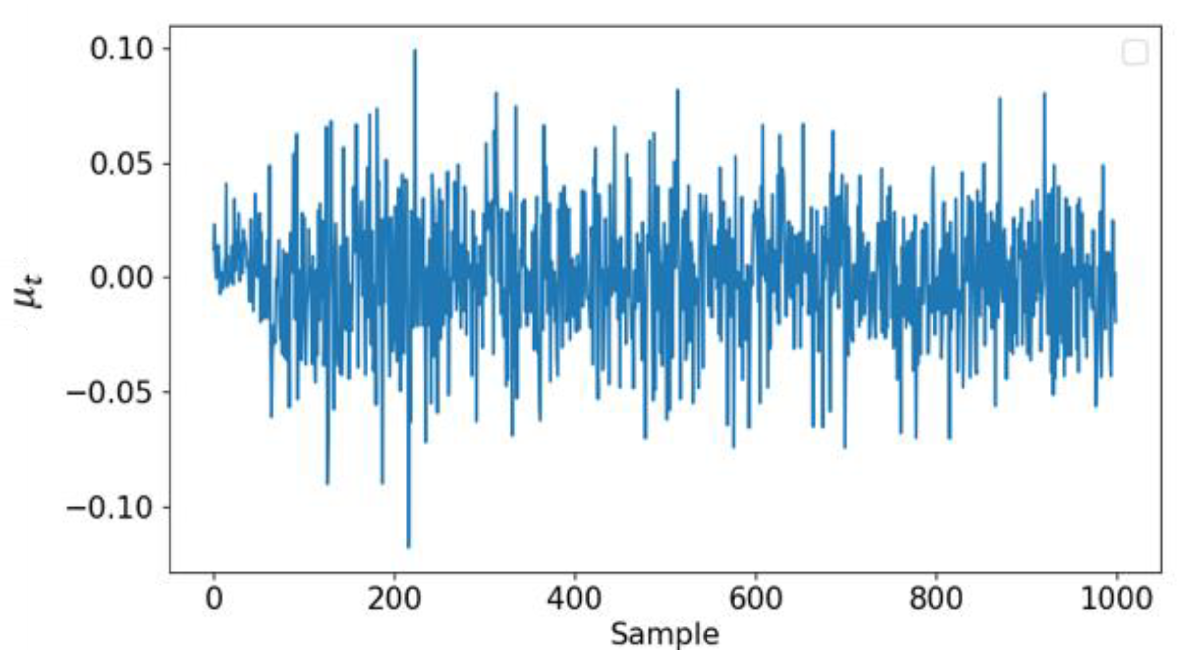
Step 4: Construct the monitoring statistics T τ 2 and control limit C so that online data can be monitored.

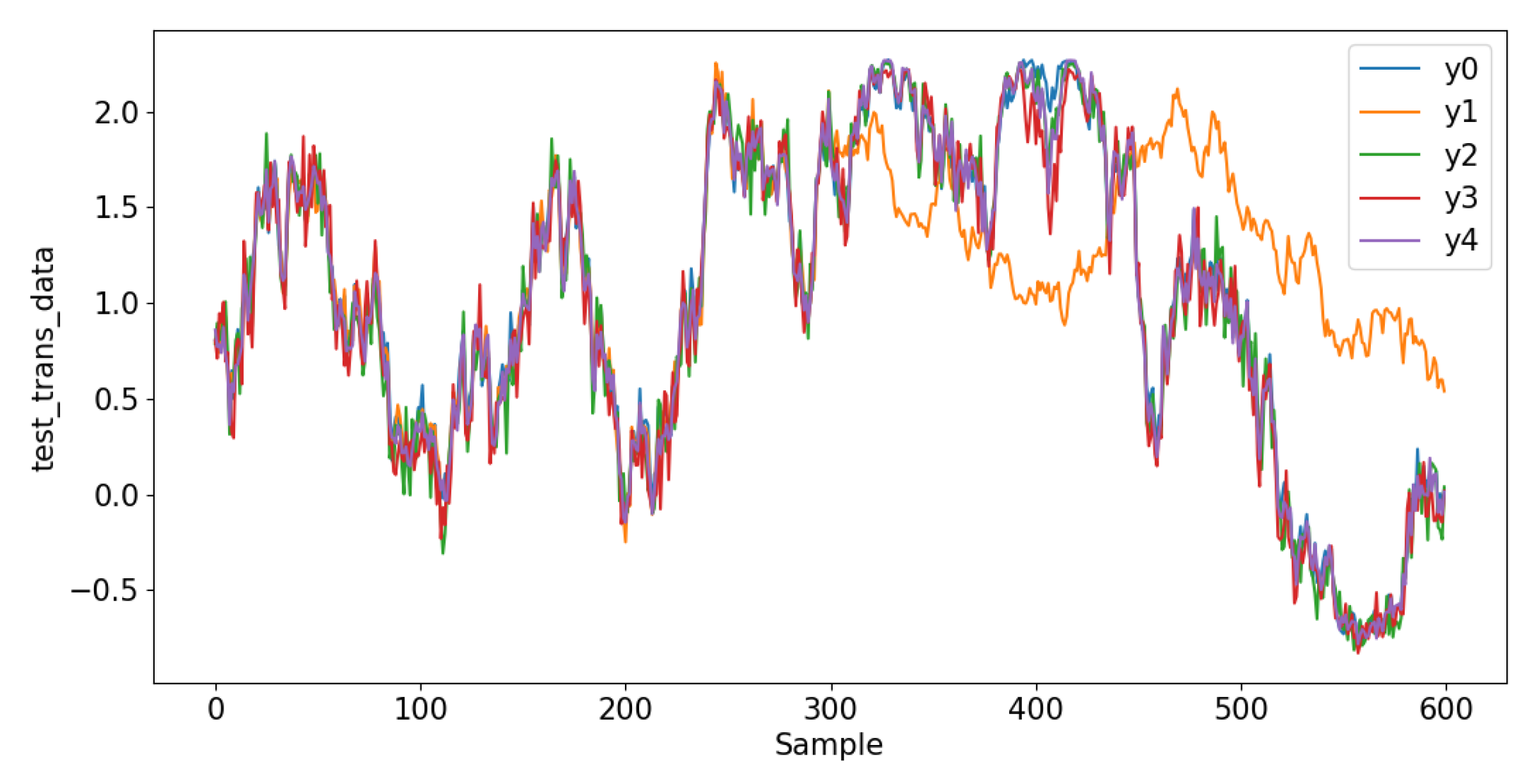
3.2. Online Monitoring

Step 1: Select the I ( 1 ) variables determined by the training data as the model input variables.
Step 2: Transform variables by the nonlinear transformation equations in step 2 above.
Step 3: Normalize the transformed variables by the process variables calculated in step 3 above. Project the transformed variables onto the cointegration coefficient matrix obtained in step 3 above:
ξ n e w = B X t n e w ,
Step 4: Construct monitoring statistics   T τ n e w 2 . When the monitoring statistics exceed the control limit C , the system will trigger an alarm.

4. Case and Result

4.1. Two-Dimensional Simulation Case

4.1.1. Data Construction

In order to verify whether the two sets of sequences f ( Y t ) and g ( X t ) transformed by the ACE algorithm are cointegrated, the following nonstationary variables X and   Y are constructed.
a t = a t 1 + e 1 t ,
x t = 0.01 a t 2 + e 2 t ,
y t = a t + e 3 t + 3 ,
where   a 0 = 0 ,   e 1 t ~ N ( 0 , 1 ) , e 2 t , e 3 t ~ N ( 0 , 0.5 ) . The total number of samples is 1000, and X and Y are shown in the Figure 2:

4.1.2. ACE and EG Test

Least square regression is performed between X t and Y t , the following equation is obtained:
Y t = 17.7144 + 0.9250 X t + μ t ,
μ t is shown in Figure 3:
The ADF test shows that the series is nonstationary. The result of the EG test indicates that there is no cointegration relationship between X t and Y t . The constructional data after ACE is shown in Figure 4:
Least square regression is performed between X t t r a n s and Y t t r a n s , the following equation is obtained:
Y t t r a n s = 1.4844 × 10 11 + 1.00024 X t t r a n s + μ t ,
μ t is shown in Figure 5.
The ADF test shows that the series is nonstationary. The result of the EG test indicates that the transformed data are cointegrated. It is proved that the ACE algorithm can transform two non-cointegration variables into cointegration variables.

4.2. Multidimensional Simulation Case

4.2.1. Data Construction

To verify the effectiveness of the proposed monitoring method, a set of simulation variables is constructed as follows:
x t = x t 1 + e 1 t ,
y 0 t = 0.02 x t 2 + e 2 t ,
y 1 t = x t + e 3 t ,
y 2 t = 0.01 x t 2 + e 4 t 10 ,
y 3 t = 0.01 x t 2 + e 5 t + 4 ,
y 4 t = 0.03 x t 2 e 6 t 20 ,
where   e 1 t ~ N ( 0 , 1 ) , e 2 t , e 3 t , e 4 t , e 5 t , e 6 t ~ N ( 0 , 0.5 ) , x 0 = 0 . The total number of samples is 1600 and the training data sample are shown in Figure 6:
Figure 6 shows that trends of these variables are roughly the same. At the 300th sample of the test data, a fault is introduced to y 1 to break the long-term equilibrium relationship between variables. After 300 samples, y 1 is constructed as follows:
y 1 t = y 1 t 1 + e t ,
where e 1 t ~ N ( 0 , 0.5 ) , y 1 changes as shown in the Figure 7, where the solid line indicates normal data and the dotted line indicates fault. After the fault is introduced, the long-term equilibrium trend no longer exists between y 1 and other variables.

4.2.2. ACE and Johansen Test

Transformed data by ACE are shown in Figure 8:
The following quartic polynomial fitting on the transformed data is performed to obtain the nonlinear transformation function, and the results are shown in Table 1.
f ( x ) = A x 4 + B x 3 + C x 2 + D x   + E ,
The test data are transformed through the equation above.
In Figure 9, it can be observed that the change trend of the training and test data is the same in addition to the fault data, so that the Johansen test can perform well. The Akaike information criterion is used to determine the lag order of the VAR model, which is calculated as 2. Table 2 shows the results:
Table 2 shows the results of the Johansen test with ACE, while the results of Table 3 are obtained without ACE transformed. At the 5% significance level, the assumption that r 3 is acceptable in Table 1. The number of cointegration relationship is 3, that is, there are three forms of linear combination that can eliminate the nonstationary trend among these variables.
However, in Table 3, the assumption that r 2 is acceptable. It shows that there are more cointegration relationships among variables after ACE algorithm transform.

4.2.3. Monitoring Results

The monitoring results based on common cointegration and the method proposed in this paper are shown in Figure 10 and Figure 11:
The blue solid line represents the monitoring statistics, and the red horizontal solid line represents the monitoring control limit. If the statistics exceed the control line, it is considered to be in an abnormal state. It can be observed from Figure 10 and Figure 11 that the monitoring method based on common cointegration analysis will not trigger an alarm when a fault occurs, while the method proposed in this paper can trigger an alarm in time, which shows that the monitoring strategy proposed in this paper is more sensitive to this type of fault.

4.3. Industrial Case

4.3.1. Introduction

The pressure drop at the hot end of the heat exchanger in the catalytic reforming process unit of a petrochemical company often rises abnormally, which may lead to safety incidents if it is not handled quickly. Therefore, it is particularly necessary to monitor the process.
A section of historical data with an abnormal rise of pressure drop is selected, including 2000 sample points. The sampling frequency is 1 min, and each sample consists of 27 variables.
The pressure drop at the hot end of the heat exchanger is mainly affected by the feed rate of naphtha and circulating hydrogen. Figure 12 shows the changes of pressure drop at the hot end of the heat exchanger, naphtha feed rate and circulating hydrogen feed rate with time from top to bottom. The naphtha feed rate has been stable, while the change trend of the pressure drop at the hot end of the heat exchanger is basically the same as that of the circulating hydrogen feed. Near about the 1400th sample points (the red frame), that is, the 500th sample point in the test set, the pressure drop at the hot end of the heat exchanger shows an upward trend, while the feed rate of circulating hydrogen and naphtha changes steadily, indicating that an abnormal increase in the pressure drop at the hot end of the heat exchanger occurred near this point.
The first 900 samples are used as the training data to establish the model, and the remaining samples are used as the test set to verify the effectiveness of the method.

4.3.2. Modeling

In total, 27 variables in the training data are tested by ADF, and I (1) variables are selected to establish the monitoring model.
If the test statistic of ADF is greater than the critical value under 1% significance, the variable can be considered as nonstationary. These nonstationary variables are stationary after difference of the first order. Finally, eight variables are determined as modeling variables. The test statistic and critical value are showed in Table 4.
The relationship of some variables in training data transformed by the ACE algorithm is shown in Figure 13, where the abscissa represents the original values and the ordinate represents the transformed values.
Then the Johansen test is performed on these variables The results of the Johansen test and the Johansen test with the ACE algorithm are shown in Table 5 and Table 6.
At the 5% significance level, the assumption that r 4 is acceptable while r 3 is rejected. Thus, there are four cointegration relationships among these variables. Although both methods have tested four cointegration relationships, the trace statistics of the Johansen test processed by the ACE algorithm are larger than that of the ordinary Johansen test, which means that the ACE algorithm still has the possibility to test more cointegration relationships.

4.3.3. Monitoring Results

The control limit C is calculated with training set data, and T τ 2   statistics are calculated for test data. The monitoring results of the two methods are as follows:
It can be observed from Figure 14 that the T τ 2   statistics of the monitoring method based on conventional cointegration analysis have exceeded the control limit before the abnormal rise of the pressure drop at the hot end of the heat exchanger, and there are a large number of false alarms, which indicates that inherent features of process data are not well captured by the traditional cointegration method.
In Figure 15, the system triggers an alarm at approximately the 517th sample point, when the monitoring statistics exceed the control limit, which shows that the monitoring method based on cointegration analysis with ACE also shows a good monitoring performance in practical industrial cases, which also verify that nonlinear cointegration exists in the considered process.

5. Conclusions

In this work, a nonstationary process monitoring strategy based on CA and an ACE algorithm is proposed. Through traditional CA, only the linear cointegration relationship between variables can be extracted. As a nonparametric method, the ACE algorithm only depends on the extremely weak distribution assumption, and a variety of nonlinear transformation forms of data can be obtained, so that the nonlinear characteristics of different forms of variables can be described [24]. Thus, the nonlinear cointegration relationship can be extracted by CA combined with ACE.
Aiming at nonlinear and nonstationary industrial data, nonlinear transformation derived by ACE is first performed on non-cointegration series. These transformations converge gradually to an optimal transformation obtained through the nonparametric data smoothing technique, namely the optimal ACE transformation, which is similar to robust optimization [25,26]. If there is a certain long-term nonlinear relationship between these series, this long-term equilibrium relationship among these transformed series could be extracted by traditional CA, which means that the transformed series become cointegrated and the nonlinear and nonstationary data characteristics can be extracted.
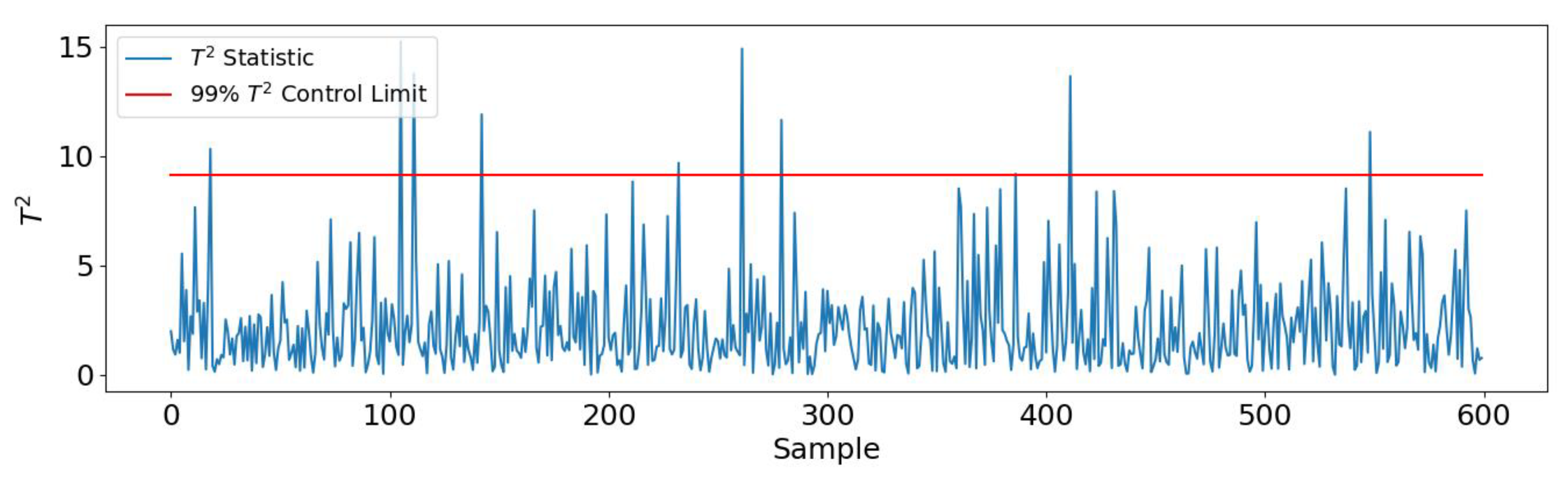
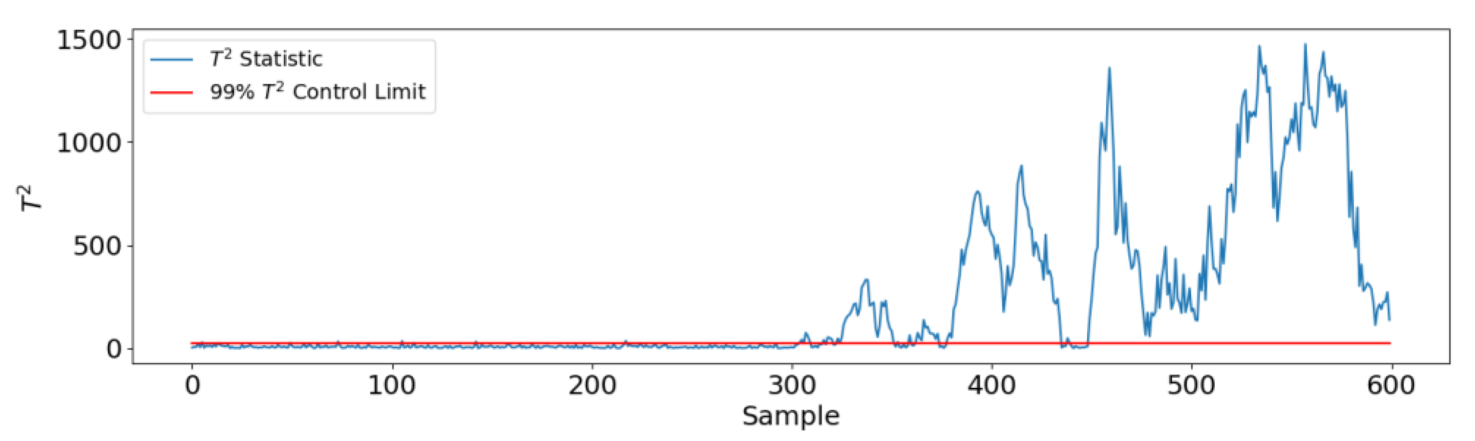
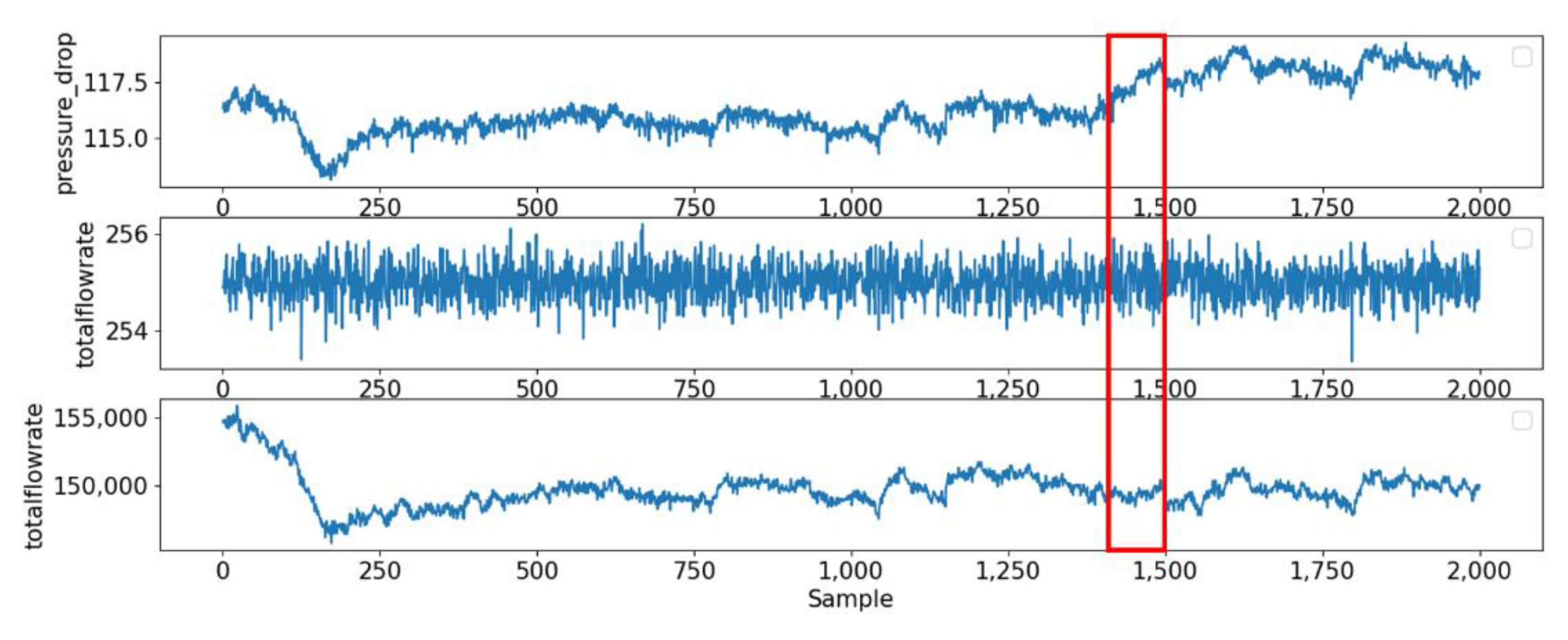
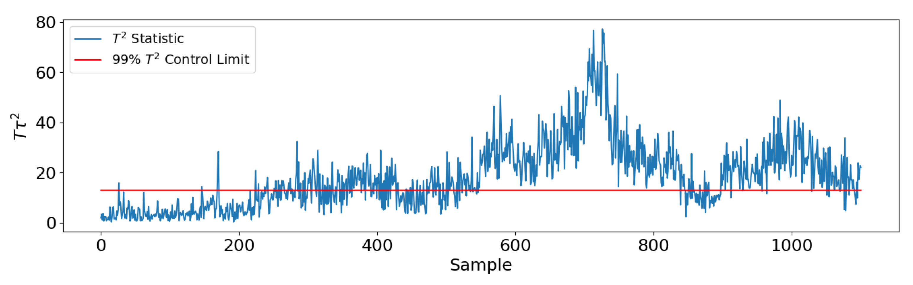
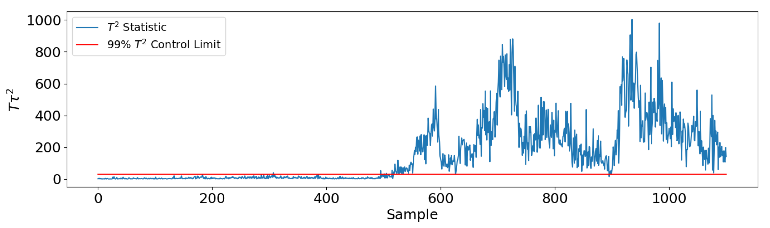
The strategy proposed is also applied in multi-dimensional simulation data and industrial data. The results show that the strategy can trigger an alarm in time when the fault occurs, while the traditional monitoring strategy based on cointegration theory results in a large number of false alarms, which means that the strategy has a wider application range and higher sensitivity.

Author Contributions

Conceptualization, J.R. and W.S.; methodology, J.R. and J.W. (Jiatao Wen); software, J.R. and J.W. (Jiatao Wen); validation, J.R.; formal analysis, J.R.; investigation, J.R.; resources, J.R., J.W. (Jingde Wang) and W.S.; data curation, J.R. and J.W. (Jingde Wang); writing—original draft preparation, J.R.; writing—review and editing, J.R., C.J. and W.S.; visualization, J.R.; supervision, W.S. and J.W. (Jingde Wang); project administration, W.S. and J.W. (Jingde Wang). All authors have read and agreed to the published version of the manuscript.

Funding

This research was funded by the National Natural Science Foundation of China (Grant No. 22278018).

Data Availability Statement

Not applicable.

Conflicts of Interest

The authors declare no conflict of interest.

References

  1. Ge, Z.; Song, Z.; Gao, F. Review of Recent Research on Data-Based Process Monitoring. Ind. Eng. Chem. Res. 2013, 52, 3543–3562. [Google Scholar] [CrossRef]
  2. Ji, C.; Sun, W. A Review on Data-Driven Process Monitoring Methods: Characterization and Mining of Industrial Data. Processes 2022, 10, 335. [Google Scholar] [CrossRef]
  3. Julieta, C.; Daniel, S.; Barbara, G. Monitoring Wine Fermentation Deviations Using An ATR-MIR Spectrometer and MSPC Charts. Chemom. Intell. Lab. Syst. 2020, 201, 104011. [Google Scholar]
  4. Tong, C.; Shi, X. Mutual Information Based PCA Algorithm with Application in Process Monitoring. CIESC J. 2015, 10, 6. [Google Scholar]
  5. Li, Z.; Liang, L.; Han, C. Multi-Rate Process Fault Detection Based on Partial Least Squares. Comput. Simul. 2016, 10, 5. [Google Scholar]
  6. Pollanen, K.; Hakkinen, A.; Reinikainen, S. Dynamic PCA-Based MSPC Charts for Nucleation Prediction in Batch Cooling Crystallization Processes. Chemom. Intell. Lab. Syst. 2016, 84, 126–133. [Google Scholar] [CrossRef]
  7. Ji, C.; Ma, F.; Wang, J.; Sun, W. Early Identification of Abnormal Deviations in Nonstationary Processes by Removing Non- Stationarity. Comput. Aided Chem. Eng. 2022, 49, 1393–1398. [Google Scholar]
  8. Ku, W.; Storer, R.H.; Georgakis, C. Disturbance Detection and Isolation by Dynamic Principal Component Analysis. Chemom. Intell. Lab. Syst. 1995, 30, 179–196. [Google Scholar] [CrossRef]
  9. Rato, T.J.; Reis, M.S. Advantage of Using Decorrelated Residuals in Dynamic Principal Component Analysis for Monitoring Large-Scale Systems. Ind. Eng. Chem. Res. 2013, 52, 13685–13698. [Google Scholar] [CrossRef]
  10. Box, G.; Jenkins, G.M. Time Series Analysis, Forecasting, and Control; John Willey & Sons: Hoboken, NJ, USA, 2015. [Google Scholar]
  11. Engle, R.F.; Granger, C. Cointegration and Error-Correction: Representation, Estimation and Testing. Econometrica 1987, 55, 251–276. [Google Scholar] [CrossRef]
  12. Granger, C. Some Properties of Time Series Data and Their Use in Econometric Model Specification. J. Econom. 1981, 16, 121–130. [Google Scholar] [CrossRef]
  13. Chen, Q.; Pan, Y. Application of Cointegration Testing Method to Condition Monitoring and Fault Diagnosis of Nonstationary FCCU System. Acta Pet. Sin. 2007, 23, 69–76. [Google Scholar]
  14. Xu, Z. Nonstationary Process Monitoring and Fault Diagnosis Using Cointegration with Structural Change Testing Method. Master’s Thesis, Nanjing University of Aeronautics and Astronautics, Nanjing, China, December 2007. [Google Scholar]
  15. Yu, W.; Zhao, C.; Huang, B. Recursive Cointegration Analytics for Adaptive Monitoring of Nonstationary Industrial Processes with both Static and Dynamic Variations. J. Process Control 2020, 92, 319–332. [Google Scholar] [CrossRef]
  16. Wen, J.; Li, Y. Nonstationary Process Monitoring Based on Cointegration Theory and Multiple Order Moments. Processes 2022, 10, 169. [Google Scholar] [CrossRef]
  17. Breiman, L.; Friedman, J.H. Estimating Optimal Transformations for Multiple Regression and Correlation. Publ. Am. Stat. Assoc. 1985, 80, 580–598. [Google Scholar] [CrossRef]
  18. Xue, G. Optimal Transformations for Multiple Regression: Application to Permeability Estimation from Well Logs. Spe Form. Eval. 1997, 12, 85–94. [Google Scholar] [CrossRef] [Green Version]
  19. Zhang, X.; Zhang, S. A Reconsideration to the Nonlinear Transformation of the Integrated Time Series. J. Syst. Eng. 1998, 13, 8. [Google Scholar]
  20. Lu, F. Complex Dynamic Engineering System Codition Monitoring Research Using Cointegration Theory. Ph.D. Thesis, Nanjing University of Aeronautics and Astronautics, Nanjing, China, November 2010. [Google Scholar]
  21. Johansen, S. Statistical Analysis of Cointegration Vectors. J. Econ. Dyn. Control 1988, 12, 231–254. [Google Scholar] [CrossRef]
  22. Johansen, S. Estimation and Hypothesis Testing of Cointegration Vectors in Gaussian Vector Autoregressive Models. Econometrica 1991, 59, 1551–1580. [Google Scholar] [CrossRef]
  23. Li, G.; Qin, S.J.; Yuan, T. Nonstationarity and Cointegration Tests for Fault Detection of Dynamic Processes. IFAC Proc. Vol. 2014, 47, 10616–10621. [Google Scholar] [CrossRef] [Green Version]
  24. Zhu, H.; Li, S.; Zeng, H. Test for Bayesian Nonlinear Cointegration in Nonparametric ACE Transformed Model. J. Manag. Sci. China 2011, 14, 52–64. [Google Scholar]
  25. Özmen, A.; Weber, G.W.; Batmaz, İ. RCMARS: Robustification of CMARS with Different Scenarios under Polyhedral Uncertainty Set. Commun. Nonlinear Sci. Numer. Simul. 2011, 16, 4780–4787. [Google Scholar] [CrossRef]
  26. Özmen, A.; Weber, G.W.; Batmaz, İ. The New Robust CMARS (RCMARS) Method. Vectors 2010, 1, 362–368. [Google Scholar]
Figure 1. Monitoring strategy based on ACE and CA.
Processes 10 02003 g001
Figure 2. Two-dimensional simulation data.
Processes 10 02003 g002
Figure 3. Residual sequence of raw data.
Processes 10 02003 g003
Figure 4. Two-dimensional transformed data.
Processes 10 02003 g004
Figure 5. Residual sequence of transformed data.
Processes 10 02003 g005
Figure 6. Training data sample.
Processes 10 02003 g006
Figure 7. Test and fault data sample.
Processes 10 02003 g007
Figure 8. Transformed train data by ACE.
Processes 10 02003 g008
Figure 9. Transformed test data through fitting curves.
Processes 10 02003 g009
Figure 10. Monitoring results of common cointegration analysis.
Processes 10 02003 g010
Figure 11. Monitoring results of cointegration analysis with ACE.
Processes 10 02003 g011
Figure 12. Variation trend of pressure drop at hot end.
Processes 10 02003 g012
Figure 13. Ace transformation relation of the selected variables.
Processes 10 02003 g013
Figure 14. Monitoring results of industrial case based on cointegration analysis.
Processes 10 02003 g014
Figure 15. Monitoring results of industrial case based on cointegration analysis with ACE.
Processes 10 02003 g015
Table 1. Polynomial fitting coefficient table.
y 0 y 1 y 2 y 3 y 4
A3.803 × 10−7−2.346 × 10−67.105 × 10−6−5.025 × 10⁻⁷−2.341 × 10⁻⁸
B9.533 × 10−51.788 × 10−41.308 × 10−3−7.445 × 10⁻⁴−2.182 × 10⁻⁵
C4.193 × 10−3−1.713 × 10−35.973 × 10−23.087 × 10−25.489 × 10−4
D−4.106 × 10−22.945 × 10−38.172 × 10⁻¹−1.893 × 10−16.948 × 10−2
E−9.707 × 10⁻¹−8.798 × 10−12.565−5.595 × 10−16.563 × 10−2
Table 2. Johansen test results with ACE.
Johansen H0 HypothesisTrace StatisticsCritical Value (5%)
r 0 549.3533.8415
r 1 286.84415.4943
r 2 65.360629.7961
r 3 1.8536747.8545
r 4 069.8189
Table 3. Johansen test results without ACE.
Johansen H0 HypothesisTrace StatisticsCritical Value (5%)
r 0 566.013.8415
r 1 276.36215.4943
r 2 11.039529.7961
r 3 2.8958847.8545
r 4 069.8189
Table 4. Unit root test results of training data.
VariableTest StatisticCritical Value (1%)VariableTest StatisticCritical Value (1%)
Inlet flow of cold end−30.5959−3.43764Inlet temperature of hot end−4.4610−3.43765
Hydrogen flow rate−2.8303−3.43766Inlet temperature of cold end−5.0377−3.43765
Inlet pressure of cold end−3.3003−3.43766Outlet temperature of cold end−4.0436−3.43766
Hydrogen pressure−2.8968−3.43766Outlet temperature of the first furnace−15.7487−3.43766
Outlet pressure of hot end−11.3220−3.43766Outlet temperature of the second furnace−19.9573−3.43765
Pressure drops of hot end−3.1284−3.43766Outlet temperature of the first reactor−3.3998−3.43766
Pressure drops of cold end−3.4391−3.43766Outlet temperature of the second reactor−3.1017−3.43766
Pressure drops of the first reactor−3.6682−3.43766Outlet temperature of the third furnace−19.2434−3.43766
Pressure drops of the second reactor−2.8726−3.43766Outlet temperature of the third reactor−4.2464−3.43766
Pressure drops of the third reactor−3.5858−3.43766Outlet temperature of the fourth furnace−18.8509−3.43766
Pressure drops of the fourth reactor−3.8137−3.43766Temperature drops of the third furnace−9.2383−3.43766
Inlet pressure of the fourth reactor−3.8399−3.43766Temperature drops of the fourth furnace−7.7637−3.43766
Pressure drops of cold end filter−12.1079−3.43766Temperature drops of the second furnace−4.3286−3.43766
Outlet temperature of hot end−2.8410−3.43766
Table 5. Johansen test results for industrial case.
Johansen H0 HypothesisTrace StatisticsCritical Value (5%)
r 0 419.5153.8415
r 1 215.01815.4943
r 2 121.07629.7961
r 3 50.908447.8545
r 4 26.023169.8189
r 5 9.8899295.7542
r 6 2.44853125.618
r 7 0159.529
Table 6. Johansen test with ACE results for industrial case.
Johansen H0 HypothesisTrace StatisticsCritical Value (5%)
r 0 419.4863.8415
r 1 250.8215.4943
r 2 161.23229.7961
r 3 96.628847.8545
r 4 54.898469.8189
r 5 20.835395.7542
r 6 6.35215125.618
r 7 −0159.529
Publisher’s Note: MDPI stays neutral with regard to jurisdictional claims in published maps and institutional affiliations.

