1. Introduction
Bitcoin is a peer-to-peer electronic currency system that does not rely on any centralized authorities. Indeed, different from traditional currencies, the Bitcoin system is based on a network of users which build a replicated ledger and mutually verify transactions. Since its inception in 2009, Bitcoin paved the way for the world of cryptocurrencies, which now number as many as 5025 cryptocurrencies as of 13 January 2020. However, Bitcoin still preserves its dominant position, both in terms of market capitalization and notoriety. Given its innovative nature, it has received considerable attention among academics, analysts, and policymakers during the last decade.
The predictability of the Bitcoin price dynamics is surely one bullet point which deserves to be studied. That is the reason why several researches have empirically detected the main features of the Bitcoin market, focusing on
Malkiel and Fama (
1970), Efficient Market Hypothesis (EMH).
Urquhart (
2016) inspected the existence of the weak form of EMH in Bitcoin returns by applying six different i.i.d. tests over the timeframe ranging from 1 August 2010 to 31 July 2016, with subsamples from 1 August 2010 to 31 July 2013 and 1 August 2013 to 31 July 2016.
Urquhart (
2016) concludes that the Bitcoin market is not weakly efficient over the full time period, with some evidence of weak form efficiency in the last subsample, which leads to the conclusion that the Bitcoin market might be moving towards efficiency. Later,
Nadarajah and Chu (
2017) extended the analysis of
Urquhart (
2016) by applying eight different tests on an odd integer power transformation of Bitcoin returns. They found out that Bitcoin returns were weakly efficient during their studied timeframe.
Bariviera et al. (
2017) investigated some statistical properties of Bitcoin returns from 18 August 2011 to 15 February 2017, at different time scales, via the Hurst exponent by means of the Detrended Fluctuation Analysis method, using a sliding window in order to study the dynamics of long-range dependence properties of the Bitcoin price. This analysis shows evidence of persistency (procyclicality) in the time series of the Hurst exponent from 2011 to 2014. Furthermore, they found that after 2014 the Bitcoin market became more informationally efficient.
Tiwari et al. (
2017), by means of computationally efficient long-range dependence estimators, showed that the market was informationally efficient, reaching consistent conclusions with respect to the results of
Urquhart (
2016),
Nadarajah and Chu (
2017), and
Bariviera et al. (
2017).
Jiang et al. (
2018) investigated the time-varying long-term memory in the Bitcoin market, using the Generalised Hurst Exponent. Such a time-varying approach is useful in tracking the dynamic efficiency of the market. Moreover,
Brauneis and Mestel (
2018) proposed a measure to test the efficiency of the market and found evidence that the market becomes less inefficient as liquidity increases. They also showed that Bitcoin complies with more statistical tests for randomness in returns than other cryptocurrencies over their analyzed time period, which ranged from 31 August 2015 to 30 November 2017.
Comparing the time-varying weak-form efficiency of Bitcoin prices in terms of US dollars (BTCUSD) with those in euros (BTCEUR), at a high-frequency level,
Sensoy (
2019) found that both markets have become more informationally efficient at the intraday level since the beginning of 2016, and the BTCUSD market was slightly more efficient than the BTCEUR market in the sample period. Furthermore, an interesting additional finding is that the higher the frequency, the lower is the pricing efficiency. Finally, they showed that liquidity (volatility) has a significant positive (negative) effect on the informational efficiency of Bitcoin prices.
Jain et al. (
2019) studied returns and volume commonalities across Bitcoin and fiat currencies. Their findings suggest that trading volumes exhibit commonality across Bitcoin and fiat currencies, as well as that the Bitcoin trading volume directly relates to its volatility and returns. Moreover, Bitcoin tends to appreciate during weekdays outside local working hours, while it depreciates during local working hours.
A stream of literature deals with how macroeconomic news surprises and search queries are related to Bitcoin price movements.
Al-Khazali et al. (
2018) studied the impact of macroeconomic news surprises on the returns and volatility of Bitcoin versus gold. They found that gold mostly reacts to macroeconomic news surprises as a safe-heaven, while Bitcoin behaves dissimilarly in most of the cases.
Kristoufek (
2013) found evidence that search queries on Google Trends and Bitcoin prices are connected, as well as there is a high asymmetry between the effect of increased interest in the currency when the currency is below or above its trend value.
Another field of investigation studies price discovery and interconnectedness among Bitcoin exchanges.
Brandvold et al. (
2015) studied price discovery on seven Bitcoin exchanges and found that MtGox and BTC-e were the leaders in the price formation process during the period ranging from April 2013 to February 2014. However, these exchanges were then shut down after hack attacks.
Pagnottoni and Dimpfl (
2018) showed that, over their studied timeframe, price discovery was mostly influenced by the Chinese exchange OKCoin, and they discovered that Bitcoin prices were not significantly affected by fiat currencies.
Giudici and Pagnottoni (
2019a,
2019b) examined interconnectedness and price discovery across Bitcoin exchange platforms and found that most influential platforms in the context of the price formation process and spillovers are both time and frequency dependent. Interconnectedness measures, in particular network metrics, related to cryptocurrencies were also employed by
Giudici et al. (
2020), who built an extension of the traditional Markowitz model to enhance cryptocurrency portfolio management. Furthermore,
Agosto and Cafferata (
2020) explored the co-explosiveness of the cryptocurrency market through a unit root- testing approach, highlighting a significant relationship in the explosive behavior of cryptocurrencies.
Related to the previous field, some researchers investigated the relationships existing across cryptocurrencies and other traditional assets and major currencies.
Ji et al. (
2018) studied relationships among Bitcoin and other assets via directed acyclic graphs. Their contemporaneous analysis highlights that Bitcoin is quite isolated, whereas lagged relationships with other assets subsist, in particular when Bitcoin experiences down market periods.
Bouri et al. (
2018) explored how the Bitcoin price is affected by non-linear, asymmetric and quantile effects impounded in the prices of gold and aggregate commodity indexes. They concluded that it is possible to predict Bitcoin price movements by means of price information from the aggregate commodity index and gold prices.
Hu et al. (
2019) analyzed returns from more than 200 cryptocurrencies as well as ICOs. They found that there is a large degree of skewness and volatility in returns and that Bitcoin returns act as risk factors themselves, being highly correlated with many altcoins.
Kristjanpoller and Bouri (
2019) investigated asymmetric cross-correlations existing between major currencies and cryptocurrencies. They concluded that Bitcoin and Litecoin show a high multifractal behavior, while Monero and Ripple showed a low multifractal behavior.
Another important strand of literature dealing with the price discovery and predictability of Bitcoin features is the one considering the role of trading volume in predicting Bitcoin and other cryptocurrency returns and volatility. The research conducted by
Balcilar et al. (
2017) employed a non-parametric causality-in-quantiles test to analyze the causal relation between trading volume and Bitcoin returns and volatility. The test supports that volume can generally predict returns, but not during bear and bull market periods, highlighting the importance of accounting for non-linearity and tail behavior in this context.
El Alaoui et al. (
2019) investigated, by means of the multifractal detrended cross-correlations analysis, price-volume cross-correlations in the Bitcoin market from 17 July 2010 to 2 May 2018. Results showed that the Bitcoin market lacks efficiency, as returns and changes in trading volume are linked by an underlying non-linear relationship.
A stream of literature closely connected to the price prediction concerns the opportunities coming from the Bitcoin trading.
Aalborg et al. (
2019) found that changes in Bitcoin price are unpredictable and realized volatility is highly predictable from its past values and, in this respect, they claimed Bitcoin’s behavior is similar to that of other financial assets. However, an additional finding which is not usually reported for other financial assets is that the trading volume of Bitcoin improved predictions of Bitcoin volatility.
Eross et al. (
2019), instead, examined the intraday interaction between returns, volume, bid-ask spread and volatility, using an intraday time series, aggregated to the 5-min frequency, from 1 November 2014 to 31 October 2016. A negative relationship between returns and volatility and a positive relationship between volatility and volume were found according to the Granger causality tests. To examine the impact of futures trading on the liquidity of the Bitcoin spot market,
Shi (
2017) constructed non-parametric and model-based volatility measures, showing that at least within a short period, Bitcoin futures trading played a positive role in stabilizing the spot price volatility and improving the spot market liquidity.
Pagnottoni (
2019) showed that options written on Bitcoin are systematically overpriced when considering conventionally accepted option pricing methods, highlighting market inefficiency, also at an option market level.
Gerritsen et al. (
2019) paved the way to the study of profitability of technical trading rules in the Bitcoin market. They used daily price data over the period July 2010 to January 2019 and show that the trading range breakout rule consistently delivered higher Sharpe ratios than a buy-and-hold strategy for the full sample period and during periods of strongly trending markets. Furthermore, their results suggest that other technical trading rules do not outperform the Buy and Hold (B&H) strategy.
Following
Gerritsen et al. (
2019), we were interested in comparing several widely employed technical trading rules with the B&H strategy from both daily and intraday trading on Bitcoin. We applied trend-following as well as mean reverting strategies on the Bitcoin price series, sampled at both five-minute and daily frequency, spanning the period 1 January 2012 to 20 August 2019 with a moving window of length three months, in search of profitable short and mid-term trends. Our research question concerns whether it is possible or not to beat the B&H strategy in either daily or the intraday time frame by means of proper technical analysis tools.
Our contribution to the existing literature is mainly threefold. First, we examine performances of both trend-following and mean-reversal indicators on the Bitcoin price series. Indeed, the literature currently takes into account only trend-following trading rules (see
Gerritsen et al. 2019). Second, we take into account eventual scalping activities concerning the Bitcoin market, given that we studied both performances on a daily and intraday basis. Finally, the performance related to the analyzed trading rules is evaluated through a conspicuous number of performance indicators, which considerably strengthens the conclusions drawn.
Results suggest that, over the considered period, trades on a daily basis are more profitable than intraday ones. Indeed, the B&H strategy used as benchmark outperforms the competing alternatives on an intraday basis, whereas, on a daily basis, Simple Moving Averages (EMAs) achieve the best results. We also interpret our findings on daily data as a lack of market efficiency, as the capability of strategies built on the technical analysis to generate extra-profits are often interpreted in the literature as a signal of margins for competing advantages.
The paper proceeds as follows.
Section 2 illustrates the basic features of the examined trading strategies.
Section 3 describes the data and explains how to build Technical Analysis strategies on them using some sketch examples on very short time-windows for illustrative purposes.
Section 4 provides and discusses the main results.
Section 5 concludes.
2. Technical Analysis and Trading Strategies
Technical analysis aims to identify trading opportunities by exploiting price trends and patterns that emerge from the time series of securities. As a matter of fact, many traders agree on the effectiveness of these techniques to build trading strategies, both for the soundness of underlying concepts and for the simplicity of implementation. Among the different categories, strategies coming from the technical analysis sphere can be divided into trend-following and mean reverting strategies.
Trend-following strategies (TFs) are strategies trying to take advantage of the general trend of the market. A prominent example is provided by the Buy and Hold (B&H) strategy. Following this strategy, the trader actively selects the assets to invest into at time
t = 0 and, after that, he is not concerned any more about price fluctuations and maintains the position along the whole length of the investing horizon. Let us denote by
Pt the price level at time
t, and by
rt the corresponding continuous return, i.e.,
rt =
log Pt/
Pt−1. Then, the payoff given by the B&H strategy is:
where
T represents the length of the investing horizon. This is an example of passive asset management strategy, arguably the simplest one, as the trader only selects the type and quantity of assets to detain and then does not change his position, regardless of fluctuations linked to asset prices and their related technical indicator.
Among the widely employed types of TFs, we also find Moving Averages (MAs). They evaluate the price mean value in a period of fixed length, spanning the data with a sliding window, and eliminating intrinsic noise due to fluctuations. Formally, assume to have
T observations for a given asset, and set the amplitude of the window to
k. In general,
k is a positive integer that cannot exceed the threshold [
T/2], where [.] denotes the integer part operator. Then, the MA of length
k at a generic time
t is given by:
where
is the price weight. When
equals one, the formula above returns the so-called Simple Moving Average (SMA), whereas in all other cases it returns the Weighted Moving Average (WMA). Furthermore, a slight modification of the previous expression yields the Exponential Moving Averages (EMA), namely:
where
λ is a smoothing constant. By construction, Equation (3) is recursive and assigns more weight (and hence more importance) to recent price levels rather than past ones. In other words, all the previous
k prices concur in defining
, however, the contribution of each price diminishes as we move back in time.
In general, both MA and EMA are combined to price levels in order to generate a trading rule. We might imagine generating a buying signal (+1) when the MA (EMA) crosses the price level from below, and a selling signal (−1) when it crosses the price level from above. Ex-post, if the sign of the signal is the same as that of the price fluctuation, we will get a positive return, the contrary applies when they are not concordant. If we denote by
the ±1 signal, the resulting payoff from MA and EMA strategies is therefore given by:
Different from TFs strategies, mean-reversion strategies (MRs) based on mean-reversion aim at identifying overbought (oversold) situations of securities. Among the most widely employed techniques, we find the Bollinger Bands (BBSs) and the Relative Strength Index (RSI).
BBs are bands plotted h standard deviations away from an SMA and provide at least two kinds of information to traders. First, as they depend on the volatility of returns, the bands widen during volatile periods, and squeeze when the volatility decreases. Second, as the bands wrap around the price level, when this is closer to the upper BBs bound, we are also near to being overbought in the market; on the contrary if the price maintains near the lower BBs bound, this is an indication of oversold in the market. In both cases, the closeness of the price to one of the BBs bounds indicates that the market is in proximity of a change in direction.
Wilder (
1978) proposed the RSI, which goes back in time for
k time units to compare the magnitude of related gains and losses. In other words, the RSI can be mathematically expressed as:
with:
By construction, RSI ranges from a minimum of 0 to a maximum of 100. It is conventionally accepted by traders to use certain thresholds in order to generate signals. In particular, the most widely employed threshold values are 70 and 30, which indicate that we are in an overbought or oversold stage of the market, respectively. In both cases, when the RSI level is close to the upper and lower threshold values, it means that the market is also arguably close to a reversal: The trader should then take proper actions to make profitable trades and/or hedge against losses. Additionally, in the case of reversal strategies, the payoff function takes the form discussed for the family of moving averages in Equation (4).
3. Data Description and Empirical Results
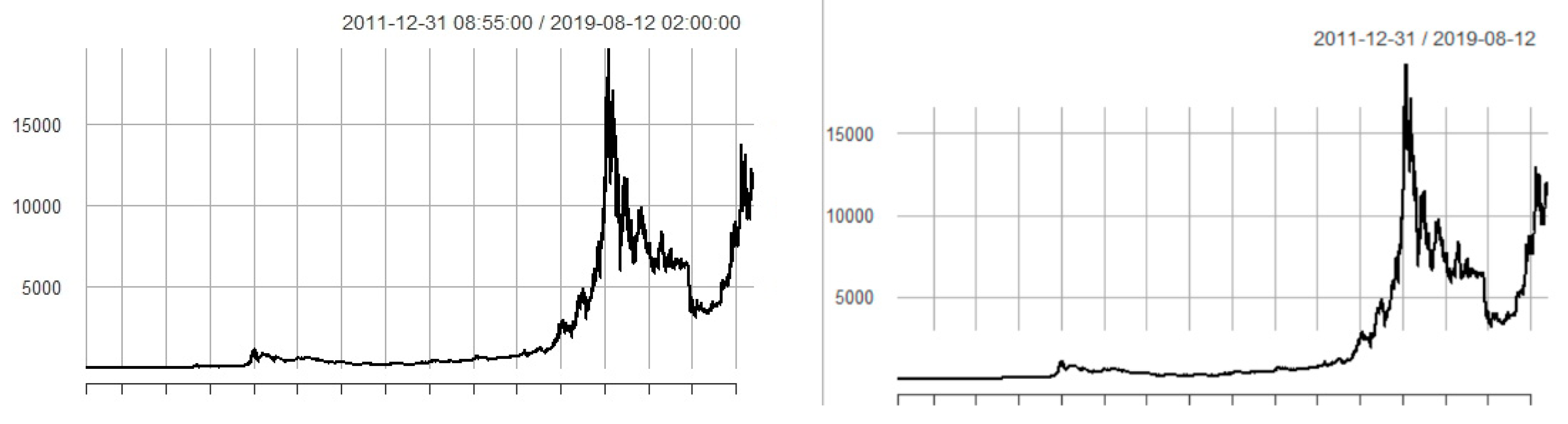
We analysed Bitcoin price series over the period ranging from 1 January 2012 to 20 August 2019; using HLOC (HLOC is the acronym for High, Low, Open and Close price levels) timeseries freely available on the Kaggle website (
https://www.kaggle.com/). We dealt with data sampled both at five-minute intervals (Btc5min) and on a daily basis (Btc1d), counting 800,834, and 2779 observations respectively. The dynamics of both price series is shown in
Figure 1. Obviously, the graphs show similar patterns, as we are dealing with the same time series but sampled at different intervals; however, the 5-min interval time series is more detailed, whereas the daily one is more rounded than the other. Their similarity is also confirmed by the summary statistics provided in
Table 1, where we examined basic features of the data.
Overall, the Bitcoin price series maintained as quite stable, with limited fluctuation in the period 2012–2015 and then witnessed a substantial growth with corrections. In fact, after a growing period between 2015 to December 2017 of notable strength especially between mid-September and the end of December 2017, the Bitcoin price started to decline and heavily fluctuated until the end of the analyzed period, namely 20 August 2019. The high dispersion of the Bitcoin is highlighted by the values of the Standard deviation (Std). Both the datasets are positively skewed; not surprisingly, the datasets exhibit leptokurtosis.
Provided with this high volatility of Bitcoin prices—and, in general, cryptocurrency—our aim was to investigate which were the most profitable trading strategies to be applied in such a context. Moreover, we wanted to understand whether the trading rules we applied were more effective when operating in an intraday setting or, given the high volatility discussed above, when trading on a daily frequency. Indeed, the latter might be still a better decision, given that sometimes it is safer to generate trading rules on a daily frequency when price changes are immediate and of high magnitude.
We generated trading strategies based on the TFs and MRs instruments described in
Section 2. In particular,
Table 2 illustrates the technical analysis tools we made use of in the current analysis describing their major features, the family to which they belong (trend-following or trend-reversal), the frequency at which we analyzed them and eventual parameters used for their computations. We applied them to the data using a sliding window of length 3-month. The rationale has its roots in Technical Analysis motivations, as 3-months is a reasonable period to highlight (and take advantage) of both short and medium-term trends.
In detail, besides the B&H strategy, which now on works as the benchmark, we considered six trend-following and six trend-reversal tools. SMA12, SMA24, and SMA72 are Simple Moving Averages, as defined in (2), with k set equal to 12, 24, and 72, time units, respectively. This means that when considering five-minute data, they are calculated going backwards by 1 hour (i.e., 12 times 5 min) and 6 h (i.e., 72 times 5 min), while in the case of daily data they are computed by considering the previous 12 and 24 days respectively. While k = 12 defines a “fast” moving average, on the contrary k = 24, 72 define “slow” moving averages. Using different lengths for the slowest moving average depending on the data gives a common-sense explanation. Indeed, while MA24 goes backward for 24 days, that is arguably enough when dealing with daily data, it can make sense to go six hours backwards in case of the 5-min sample, given the higher frequency of the data. Similar considerations apply to EMA, BBS, and RSI. In the case of EMA we additionally specified the value for the smoothing parameter. Here we chose λ = 0.94, which is a kind of canonical value employed by financial risk management companies such as RiskmetricsTM.
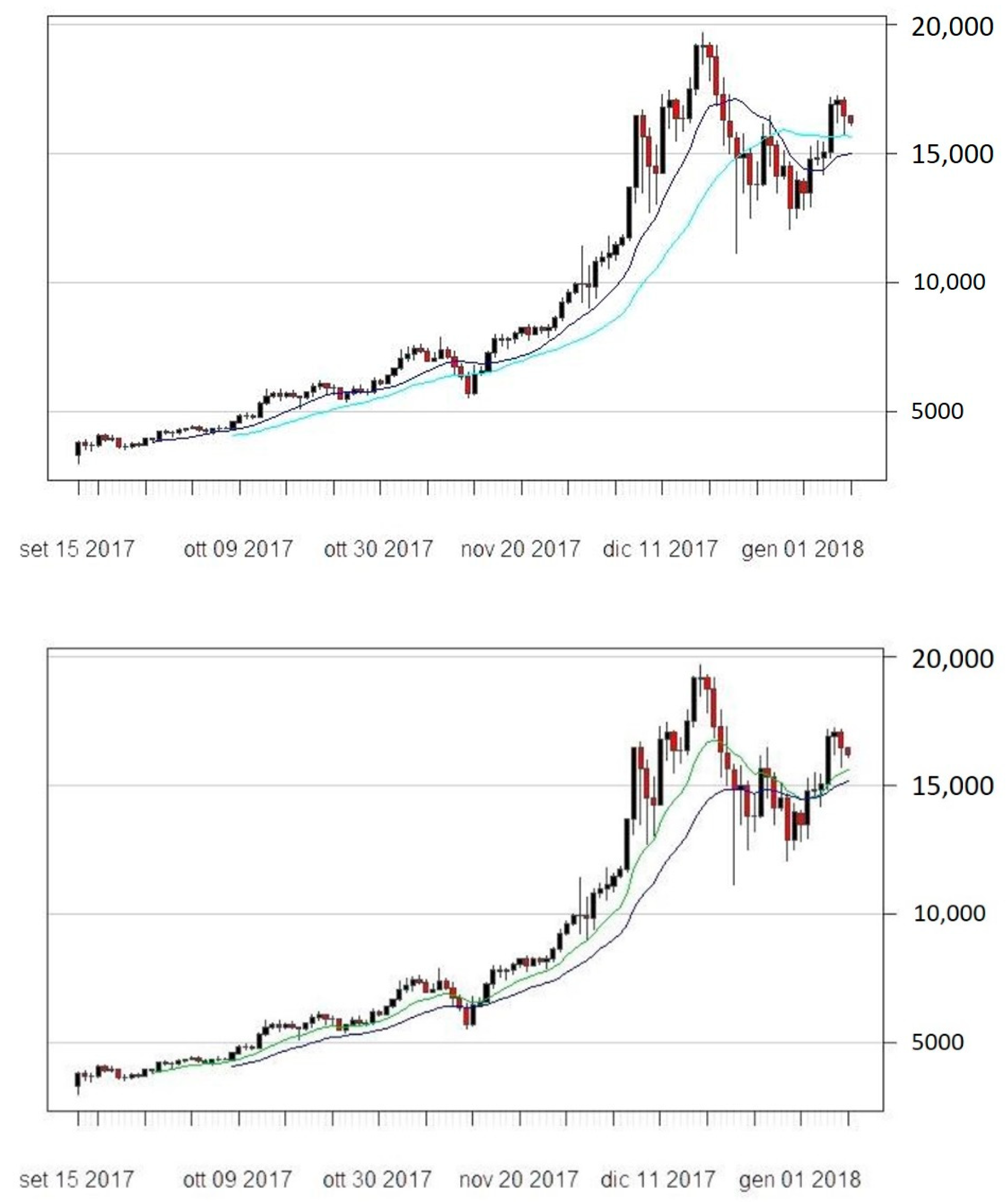
Figure 2 shows some examples of the dynamics of MA12 and MA72 on five-minute Bitcoin price series. Given the high frequency of the data, it is difficult to distinguish both the simple and exponential Mas—independently from the lag considered—from the actual Bitcoin price series. For this reason, we now offer some snapshots about the way these strategies work, focusing on a very limited time frame and plot a highlight of some of the strategies, in particular SMAs and RSIs, for the period 29 December 2017 to 3 January 2018 in
Figure 3, namely considering the last three days belonging to the year 2017 and the first three days of 2018.
In general, plots show that crossing of the MAs occurs quite often during the restricted sample considered, meaning that they generate a buy/sell signal quite frequently. Besides that, from a visual inspection one can also notice that RSI generates even more signals (of overbought or oversold) during the same period, namely crossing the 30 and 70 threshold values; this is typical of periods of high uncertainty with huge price falls following a spectacular price growth phase.
In order to assess whether performances and behaviors of the indicators are different when considering five-minutes or daily frequency, we plotted the main indicators applied to daily Bitcoin price series in
Figure 4,
Figure 5 and
Figure 6. In particular,
Figure 4 illustrates the dynamics of MA12 and MA24,
Figure 5 those of BBS12 and BBS24, while
Figure 6 those of RSI12 and RSI24.
In general, both MAs and EMAs perform quite similarly. Indeed, we may observe the presence of an upward trend in the indicators both for the MA12 and MA24. As far as BBs and RSI are concerned, they provide insightful information about the dynamic evolution of volatility in the observed timeframe. Indeed, data show a relatively low variability at the beginning of the sample period, whereas this sharply increases towards the end. In particular, this evidence is confirmed by the increasing width of the BBs over time, which is particularly marked at the beginning of the Bitcoin price hype that took place in December 2017.
4. Discussion
As far as trading strategies are concerned, we employed technical analysis to build trading rules as follows. We worked on the data with a three-month sliding window, for an overall number of 31 quarters, plus a residual two-month window covering July and August 2019 and we applied in each of them TA, using the results of the B&H strategy as benchmark. In detail, in the case of TFs, every time the MA (EMA) crosses the price level from below a buy (+1) signal is generated, whereas whenever the price level is crossed from above a sell signal (−1) occurs. For both the BBs and RSI, instead, a buy (sell) signal occurs every time the index reaches the oversold (overbought) threshold level, meaning whenever it crosses the lower (upper) band for BBs and whenever it reaches the level of 30 from above (70 from below) for RSI.
For each strategy we provided a set of downside risk metrics and spread performance measures as described in
Table 3. For explanatory purposes, we adopted the following conventions: the symbol
=
log Pt/
Pt−1 denotes the average rate of return,
T is the period length,
s is the standard deviation in the adopted time unit (daily/intraday), 1 is the indicator function,
xH the highest observed return,
q is a threshold value, with
q = MAR (Minimum accepted threshold) as special case.
Results are given in
Table 4 for intraday data and in
Table 5 for daily data. As far as specifications are concerned, we set the risk-free rate equal to 0 for the Annualized Sharpe Ratio and the Downside Deviation calculation, and we set the Minimum Accepted Return (MAR) to as much as 210%.
As far as intraday strategies are concerned, the B&H strategy clearly outperforms all competitive alternatives, both in terms of performance and riskiness. Indeed, both the Annualized Return and the Annualized Sharpe Ratio assume relatively high values, the first and the second being more than 16 and 5 times higher than the second best performing strategy (i.e., the EMA12), respectively. Furthermore, all metrics suggests that the riskiness of the B&H strategy is also generally lower, despite BBs achieving slightly better results in terms of Gain and Loss Deviation.
As far as strategies applied to daily prices are concerned, results change dramatically. Indeed, the B&H is not the best strategy anymore, yielding lower performances and higher risk with respect to several competing alternatives. The best strategies in terms of performances turn out to be the MAs and EMAs, with the MA12 being the one which outperforms all the others. Despite that, the MA12 is not the least risky strategy among those considered, with RSI72 being generally the one giving the best figures in terms of riskiness. However, RSI12 has also the worst performing trading rules, reporting even negative values in terms of performances.
Overall, we claim that the performance of the strategies varies according to the frequency of data used to identify opportunities for profitable trades. This also depends on the behavior of the Bitcoin price series during the considered period. Indeed, the B&H strategy performs better with respect to alternatives when considering daily data as holding the asset when its price is spectacularly growing turns out to be better than making trades by following potentially misleading signals and therefore realizing some losses besides gains. When dealing with daily data, instead, trading signals are surely less numerous and noisy and MAs, in particular the “fast” MA12, better capture the upward price trend and generate profitable trades which outperform the simple B&H strategy.
We also find that in our case trading on a daily basis is much more profitable than going intraday. As a matter of fact, the Annualized Return and the Annualized Sharpe Ratio realized by trading with daily data are sensitively higher than those achieved by using 5-min data. This further suggests that the noise impounded in the high-frequency data may produce trading signals which emerge as unprofitable ones. Moreover, our results are in line with
Gerritsen et al. (
2019), who found a consistent outperformance of the technical analysis trading rules with respect to the B&H strategy when considering daily data. We believe that, despite this being out of the scope of the present study, the use of trading volumes to integrate technical trading rules may result in more profitable strategies. Indeed, as pointed out in the literature (see
Balcilar et al. 2017), trading volume can help to predict Bitcoin returns in specific market phases. Furthermore, to the best of our knowledge, there has been no study yet exploiting methodologies that take into account the effect of destructured news as a financial signal—as, for example, those of
Cerchiello and Giudici (
2016) and
Cerchiello et al. (
2017)—concerning Bitcoin price dynamics, which could augment technical analysis to build even more profitable trades.


