1. Introduction
The launch of Bitcoin in 2009 marked a pivotal moment, propelling cryptocurrencies into the financial limelight. Presently, decentralized exchanges actively trade around 22,932 cryptocurrencies, indicative of the rapid expansion within this emerging market, as reported by
CoinMarketCap (
2023) This surge has not only seized the financial industry’s attention but also underscored the substantial impact of cryptocurrencies. Despite this heightened interest, the complete spectrum of potential applications remains insufficiently explored by researchers.
Cryptocurrencies, characterized by their departure from traditional financial norms, operate in the digital realm, free from central bank oversight, as emphasized by
Corbet et al. (
2019). Notably, experts such as (
Weber 2016;
Baek and Elbeck 2015) assert that Bitcoin aligns more closely with an asset than a conventional currency. A notable statistic reveals that approximately 69.2% of Bitcoin holdings remain inactive, highlighting investors’ preference for holding rather than utilizing them for transactions,
Hartmann (
2023). This inclination for speculation reinforces Bitcoin’s characterization as an asset primarily intended for speculative purposes rather than functioning as a conventional currency.
Classifying Bitcoin within a specific asset class poses a challenge, with
Burniske and White (
2017) confirming its emergence as a distinct asset class with unique attributes. This distinctiveness is apparent through its decentralized origin, limited supply structure, and foundational blockchain technology.
Micu and Dumitrescu (
2022) further emphasize the remarkable growth trajectory of Bitcoin and Ethereum, positioning them as significant financial instruments.
As cryptocurrencies gain popularity, they introduce challenges and opportunities, necessitating exploration by researchers, investors, and policymakers, while traditional research methods struggle to comprehend the intricate and unpredictable behaviors inherent in cryptocurrency markets. Furthermore, to address the complexities of cryptocurrency markets, our study employs a robust methodology that encompasses empirical examination of one-minute interval price data for Bitcoin and Ethereum. This approach allows us to delve deeply into the dynamics of high-frequency trading and risk assessment, offering valuable insights into the behavior of these digital assets.
The adoption of high-frequency data is not without risks, given the heightened scrutiny of cryptocurrency markets due to volatility, liquidity disparities, and susceptibility to manipulation. The focus on risk measurement leads to the Value-at-Risk (VaR) metric, a prevalent choice in this domain. Researchers, such as
Mata et al. (
2021), have identified the superiority of the Normal Inverse Gaussian (NIG) distribution in VaR estimation over multivariate generalized autoregressive conditional heteroscedastic models.
The NIG distribution assumes a crucial role in examining the influence of socially responsible dimensions on risk dynamics and predictability, as indicated by
Viviani et al. (
2019). Integrating social responsibility considerations into risk analysis positively impacts risk management and portfolio performance.
In alignment with our overarching goal of addressing the research gap and comprehensively exploring the applications of cryptocurrencies, particularly focusing on high-frequency trading dynamics and risk assessment, this paper aims to contribute to the field by:
Exploring the intricate dynamics of high-frequency trading;
Assessing the resilience and effectiveness of Value-at-Risk (VaR) as a risk assessment tool when applied to the unique dynamics of high-frequency cryptocurrency data;
Investigating the potential of the Normal Inverse Gaussian (NIG) distribution as a reliable distribution for estimating VaR, with a particular emphasis on its applicability to high-frequency data.
Risk management protocols, predominantly focused on daily data, can be extended to intraday data. This study empirically examines one-minute interval price data for Bitcoin and Ethereum from between 1 January 2017 and 25 October 2022. By employing specialized statistical techniques and constructing a portfolio, the study evaluates its ability to meet established confidence levels. The inclusion of high-frequency data, covering disruptive periods, like the global pandemic in 2020, contributes innovative insights to risk evaluation in high-frequency trading.
Through this exploration, we aim to quantitatively evaluate instances where the observed risk values surpass the estimated values, providing a deeper understanding of the precision and reliability of risk measurement in cryptocurrency markets. Ultimately, our objective is to contribute to the evolving research landscape by shedding light on the practicality and effectiveness of advanced distributional models in accurately modeling and predicting financial risk, especially within the realm of cryptocurrencies like Bitcoin and Ethereum. By explicitly stating the research gap, providing an overview of the methodology, and connecting the introduction to the subsequent literature review, we aim to offer a clearer roadmap for readers and highlight the contributions of our study.
The structure of this document follows a logical progression.
Section 2 provides an overview of the relevant literature, while
Section 3 explains the methods employed and the data collected. Progressing further,
Section 4 presents the outcomes and seamlessly transitions to
Section 5, where the conclusions and discussions converge, ultimately culminating in a coherent ending.
2. Literature Review
Bitcoin, as a pioneering cryptocurrency, wields a profound influence on the intricate realm of digital finance. This review explores pivotal research findings, emphasizing the far-reaching impact of Bitcoin and the crucial role of high-frequency data in modern financial analysis. The investigation’s foundation lies in the use of high-frequency data collected minute by minute for Bitcoin and Ethereum between 1 January 2017 and 25 October 2022.
Mahmoudi (
2022) underscores Bitcoin’s historical eminence, extending beyond intrinsic value, and influencing the valuation of other digital assets. The escalating costs of Bitcoin mining and its inherent supply scarcity initiate upward price trends. This dynamic interplay of factors attracts investors, amplifying demand, and culminating in an amplified pricing trajectory.
Ma and Tanizaki (
2022) provide insights into temporal price clustering patterns, complementing this discourse.
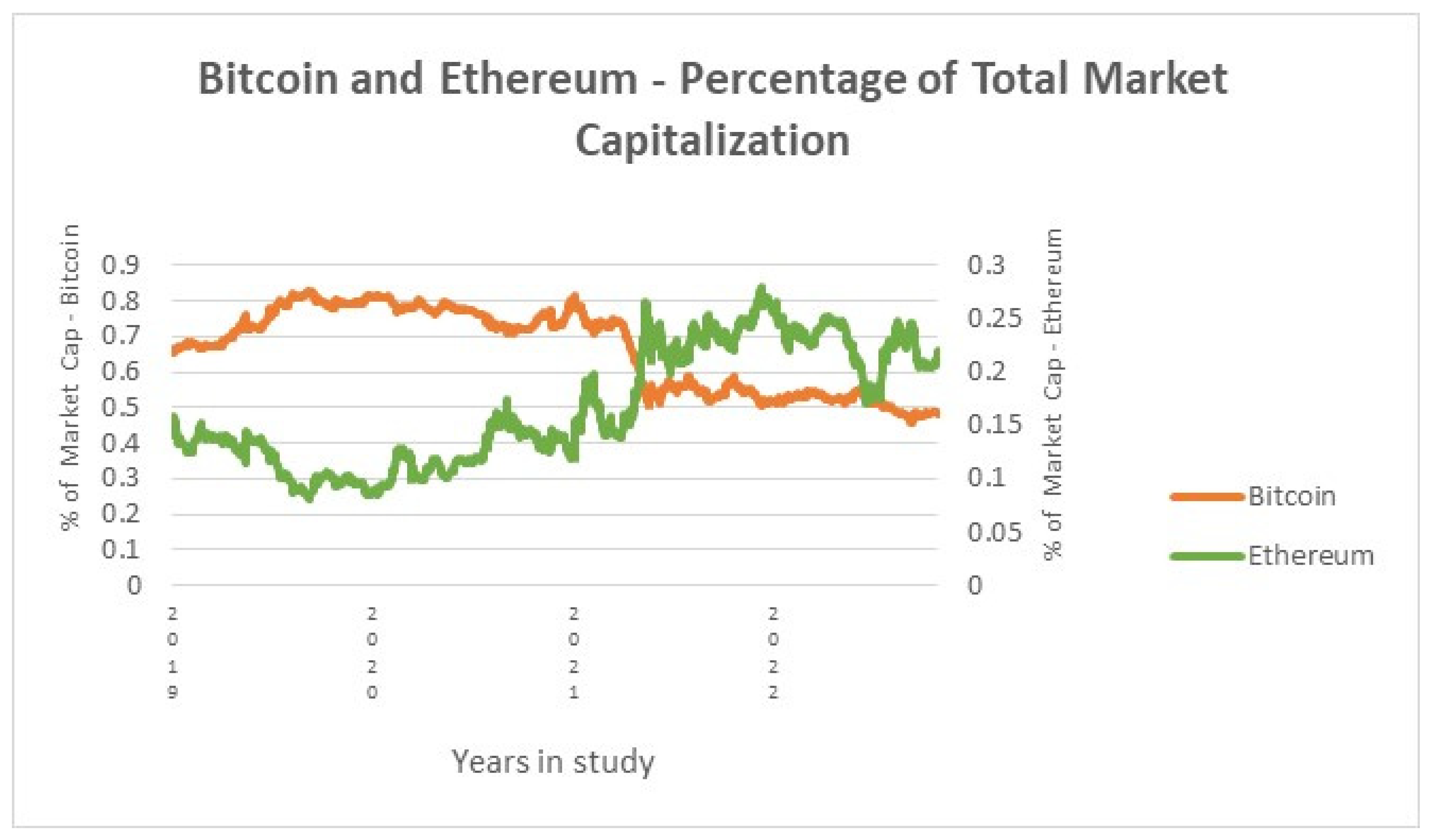
Figure 1 depicts the evolution of market capitalization for major crypto assets, consistently dominated by Bitcoin and Ethereum, affirming
Bariviera et al.’s (
2018) observation that most cryptocurrencies follow Bitcoin’s market patterns. The riskiness of Bitcoin investments is emphasized by
Zhang et al. (
2021), linking it to speculative fervor. Speculator movements during price upswings magnify trading volumes and market attention, leading to price escalations. In a broader economic context,
Zhu et al. (
2017) present empirical evidence of Bitcoin’s susceptibility to economic indicators, while
Qarni and Gulzar (
2021) highlight its role as a hedge against the US dollar and forex-related risks.
(
Blau 2017;
Chu et al. 2017;
Sahoo 2017) discuss Bitcoin’s market volatility vis-à-vis traditional fiat currencies.
Kristoufek (
2013) notes its detachment from governmental backing, preventing direct economic correlations.
Troster et al. (
2019) confirm Bitcoin’s exceptional volatility, exceeding that of traditional assets. This volatility extends to crude oil and gold markets, as evidenced by
Gronwald’s (
2019) empirical findings.
Trucíos et al. (
2020) shed light on the dichotomy of substantial returns and inherent risk exposure. The upheaval in 2020 witnessed a remarkable ascent in cryptocurrency values, a trend sustained in 2021. Bitcoin and Ethereum consistently assert their dominance, a trend acknowledged by
Miglino (
2021).
Hambuckers et al. (
2023) introduce an innovative approach through extreme value regression, offering insights into high-frequency tail risk dynamics.
Schilling and Uhlig (
2019) delve into the fundamental equilibrium pricing equation, highlighting Bitcoin’s adherence to a martingale pattern.
Liu and Tsyvinski (
2021) propose factors like momentum and investor attention for predicting Bitcoin’s returns.
Sockin and Xiong (
2020) introduce cryptocurrency valuation ratios into return prediction models.
Guindy (
2021) emphasizes investor attention in predicting price volatility, echoed by
Critien et al. (
2022) using neural models.
Zhang et al. (
2021) unveil bidirectional links between Bitcoin returns and internet attention.
Subramoney et al. (
2021) identify heavy tails in cryptocurrency returns, with the NIG distribution excelling in capturing their nature.
Ramirez-Garcia (
2022) how cases its practicality in hedging electricity price volatility.
Contreras-Valdez et al. (
2022) employ the NIG distribution in portfolio selection, affirming its efficacy and versatility.
The NIG distribution’s application in portfolio management, modeling default risk in banks
Jessen et al. (
2011), and its role in modeling risk underscore its significance. This study aims to comprehensively analyze high-frequency data and the NIG distribution in estimating VaR for Bitcoin and Ethereum, contributing insights into risk assessment within cryptocurrency markets. Through this exploration, we aim to enhance understanding and provide valuable insights for researchers, investors, and policymakers operating in high-frequency trading within the dynamic cryptocurrency landscape.
This paper’s primary objective is to comprehensively analyze the utilization of high-frequency data and the Normal Inverse Gaussian (NIG) distribution in estimating Value-at-Risk (VaR) for an evenly weighted portfolio, with a specific focus on Bitcoin and Ethereum.
Our study aims to achieve several key goals. First, we intend to assess the resilience and effectiveness of VaR as a risk assessment tool when applied to the unique dynamics of high-frequency cryptocurrency data. Second, we seek to explore the potential of the NIG distribution as a reliable model for estimating VaR, with a particular emphasis on its applicability to high-frequency data. This exploration will enable us to quantitatively evaluate instances where the observed risk values surpass the estimated values, providing a deeper understanding of the precision and reliability of risk measurement in cryptocurrency markets. Ultimately, our objective is to contribute to the evolving research landscape by shedding light on the practicality and effectiveness of advanced distributional models in accurately modeling and predicting financial risk, especially within the realm of cryptocurrencies like Bitcoin and Ethereum. Through these objectives, our study aims to provide valuable insights to researchers, investors, and policymakers, facilitating a better comprehension of risk in the context of high-frequency trading, particularly within the fast-paced and ever-changing cryptocurrency markets.
3. Methodology and Data
In this paper, we propose the estimation of a bivariate Normal Inverse Gaussian distribution designed by
Barndorff-Nielsen (
1977). A univariate version has been applied to the Bitcoin returns in
Núñez et al. (
2019). In this case, the random variable X has a Normal Inverse Gaussian density, denoted X~NIG(α,β,μ,δ) if:
A bivariate version of the NIG distribution will be used using Bitcoin and Ethereum returns. Formally, defined as:
where:
With
and
is a Generalized Inverse Gaussian variable, the density specification of which is:
Parameters (shape parameters), is the location, is the dispersion matrix, stands for the skewness parameter, and is the modified Bessel function of the third kind.
The expected Value and the Variance of the multivariate distribution of
are:
and
defines the Normal Inverse Gaussian (NIG) distribution.
For the multivariate Generalized Hyperbolic distribution, the expected value and the variance matrix are given by:
We will use the parametrization then for the NIG , , such that . With this new definition, the calculus becomes even faster from a computational perspective. We obtained the data from the Gemini Exchange, which includes intraday information with regular measurements for every minute. To create a homogeneous dataset, we computed the model from 2017 onwards for both cryptocurrencies. The dataset contains minute-by-minute closing prices of Bitcoin and Ethereum, ranging between 00:00 h on 1 January 2017 and 23:59 h on 25 October 2022.
Although the dataset was consistent enough to perform most of the models, we encountered some data cleaning requirements. The most frequently recurring issue was atypical information caused by the absence of decimal points. To prevent potential data manipulation skewness, we removed these inconsistencies from the data. The final dataset comprises the statistics presented in
Table 1.
The computation of the returns is conducted minute by minute; the descriptive statistics for each year are presented in
Table 2.
Table 2 presents significant observations regarding the kurtosis, skewness, and volatility of the Bitcoin and Ethereum returns across various years. Notably, Bitcoin’s kurtosis deviates considerably from the normal distribution value of 3, indicating heavy tails in all years. The highest kurtosis occurs in 2018, contrasting with the lowest observed in 2022, hinting at varying degrees of heavy-tailedness. These data align with the bubble observed by the end of that year. Similarly, the skewness values also fluctuate, with 2018 exhibiting the most extreme negative skewness and 2022 approaching a more normal distribution. Moreover, the volatility, measured by standard deviation, ranged between a minimum in 2022 and a maximum in 2018, with extreme statistics predominantly found in these two years.
In parallel, Ethereum’s kurtosis displays substantial variation, with 2018 recording the highest value and 2022 the lowest, signaling heavy tails akin to many financial assets. The skewness values show similar extremes in 2018 and 2022. Regarding volatility, 2017 marks the highest, while 2022 records the lowest.
It is noteworthy that the Ethereum returns exhibit consistently higher volatility compared to the Bitcoin returns across all years. These observations shed light on the dynamic statistical properties of Bitcoin and Ethereum returns, crucial for understanding their risk profiles and market behavior. These statistics clearly reveal non-Gaussian data, with the third and fourth moments deviating significantly from the normal behavior.
With this information, it becomes evident that there is a need to employ at least semi-heavy-tailed distributions to model these data. As mentioned earlier, the proposed distribution is the Normal Inverse Gaussian (NIG) due to its commendable properties. To perform the multivariate adjustment and evaluate the performance and effectiveness of this distribution, several considerations were considered. As there is a substantial amount of data, with around 1440 data points for each day, there is enough information to adjust a daily Multivariate NIG distribution. This procedure was conducted on a daily basis using a rolling window approach.
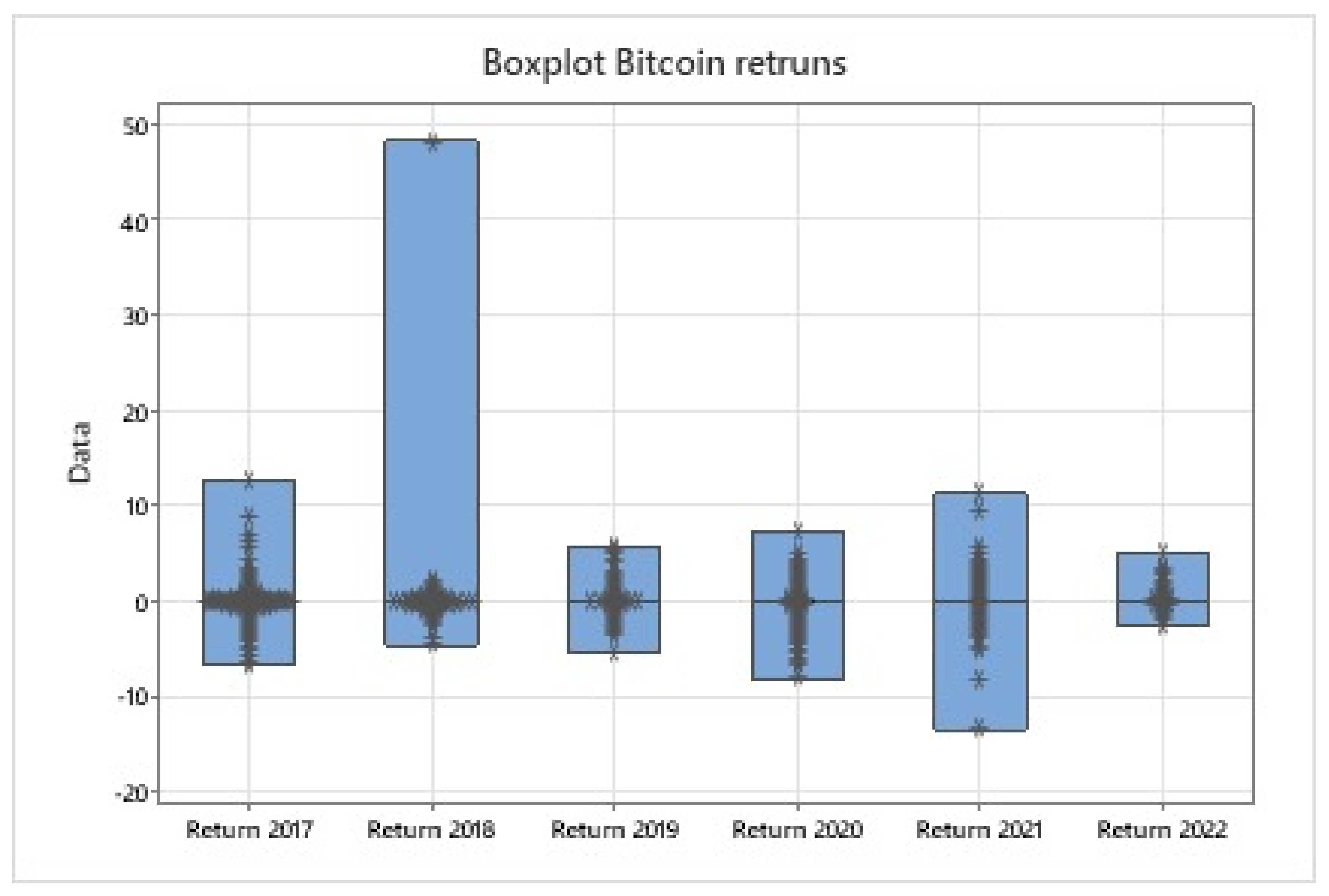
The box plots depicted in
Figure 2 reveal a notable consistency in the medians across the years 2017–2022. This aligns with the observations from
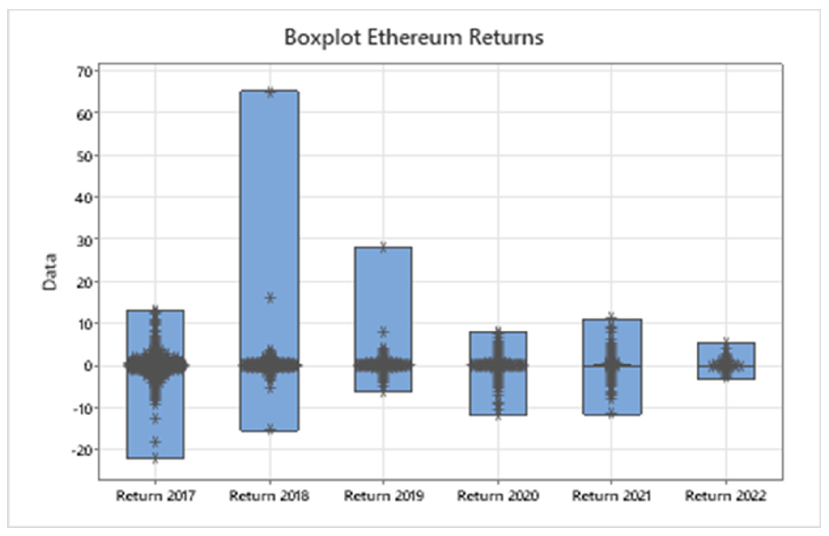
Table 2, where a similar pattern is noted for the means. Concerning the interquartile ranges, the widest dispersion is observed in 2018, whereas the narrowest dispersion occurs in 2022. Following 2018, the next significant dispersion is observed in 2021, followed by the years 2017, 2020, and 2019. In
Figure 3, the box plots for the years 2017–2022 indicate that the medians closely cluster together.
It is worth noting that on some days, the maximum likelihood algorithm did not converge due to the presence of extreme values that the distribution could not capture. The specific days that were removed are presented in
Table 3.
For these days, it is noteworthy that 2020 witnessed the highest concentration of extreme values. The initial periods coincide with the onset of the COVID-19 pandemic, while the subsequent periods are associated with the first and second waves of contagion. This phenomenon offers intriguing potential for further research and analysis.
Once the estimators for each day are calculated, these values are utilized to model the theoretical multivariate distribution for that specific day. Using these estimations, the Value-at-Risk (VaR) at a 99% confidence level is computed for an equally weighted portfolio. However, relying solely on an in-sample evaluation of the adjustment’s performance is insufficient to draw robust conclusions. To address this limitation, an out-of-sample approach was employed.
The approach involves computing the minute VaR for one day and using it as the benchmark for the following day. If the minute return for the second day exceeds the VaR computed on the first day, it is considered a failure in the estimation. The effectiveness statistic is then calculated as the percentage of minute returns that remained above the VaR. In theory, the level of effectiveness is expected to align with the chosen confidence level.
4. Results
The results align with the year-wise plots and statistics assessing the effectiveness of the Multivariate Normal Inverse Gaussian (NIG) model in capturing return behavior and volatility concerning the Value-at-Risk (VaR) statistic.
We initiated the analysis by calculating an equally weighted portfolio for each period. It is essential to note that the portfolio weights were chosen due to the high correlation among the assets, limiting the potential for proper diversification. In the conclusions section of this paper, we delve into additional considerations.
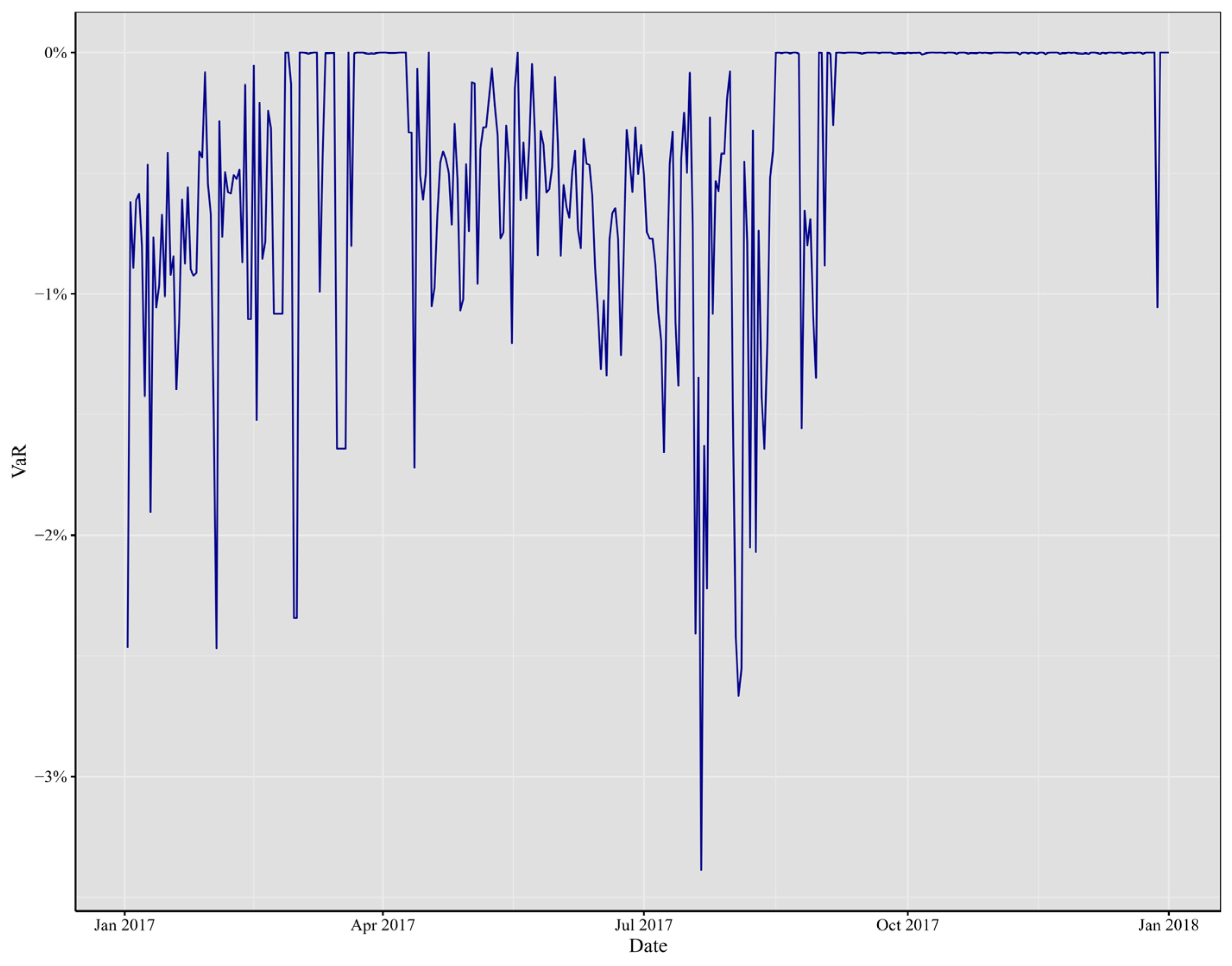
In the dynamic world of cryptocurrency, various events of different magnitude have influenced the Value-at-Risk (VaR), with Bitcoin and Ethereum remaining highly sensitive to changes, not just within financial markets, but also across the spectrum of factors, including fraud and non-financial news. Let us embark on a journey through the years, starting in 2017, through
Figure 4,
Figure 5,
Figure 6,
Figure 7,
Figure 8 and
Figure 9.
In 2017, the cryptocurrency realm bore witness to a whirlwind of impactful events. Extreme occurrences, market developments, economic announcements, and unforeseen price movements left a significant mark on minute VaR, leading to substantial alterations in its risk profile. Notable troughs were evident throughout the year, stretching from January to October, as depicted in
Figure 4. In January 2017, a substantial rally emerged, setting the stage for a trend that persisted until December. In April, an extreme trough primarily stemmed from Japan’s official recognition of Bitcoin as a legal method of payment, catalyzing increased adoption and investment within the country. Then, in June, the cryptocurrency sphere was rocked by the WannaCry ransomware attack, demanding Bitcoin payments, capturing widespread attention and shedding light on its role in cybercrime. By July, the discovery of a critical vulnerability in the Parity multi-signature wallet led to the freezing of substantial amounts of Ether, sending ripples across the Ethereum community.
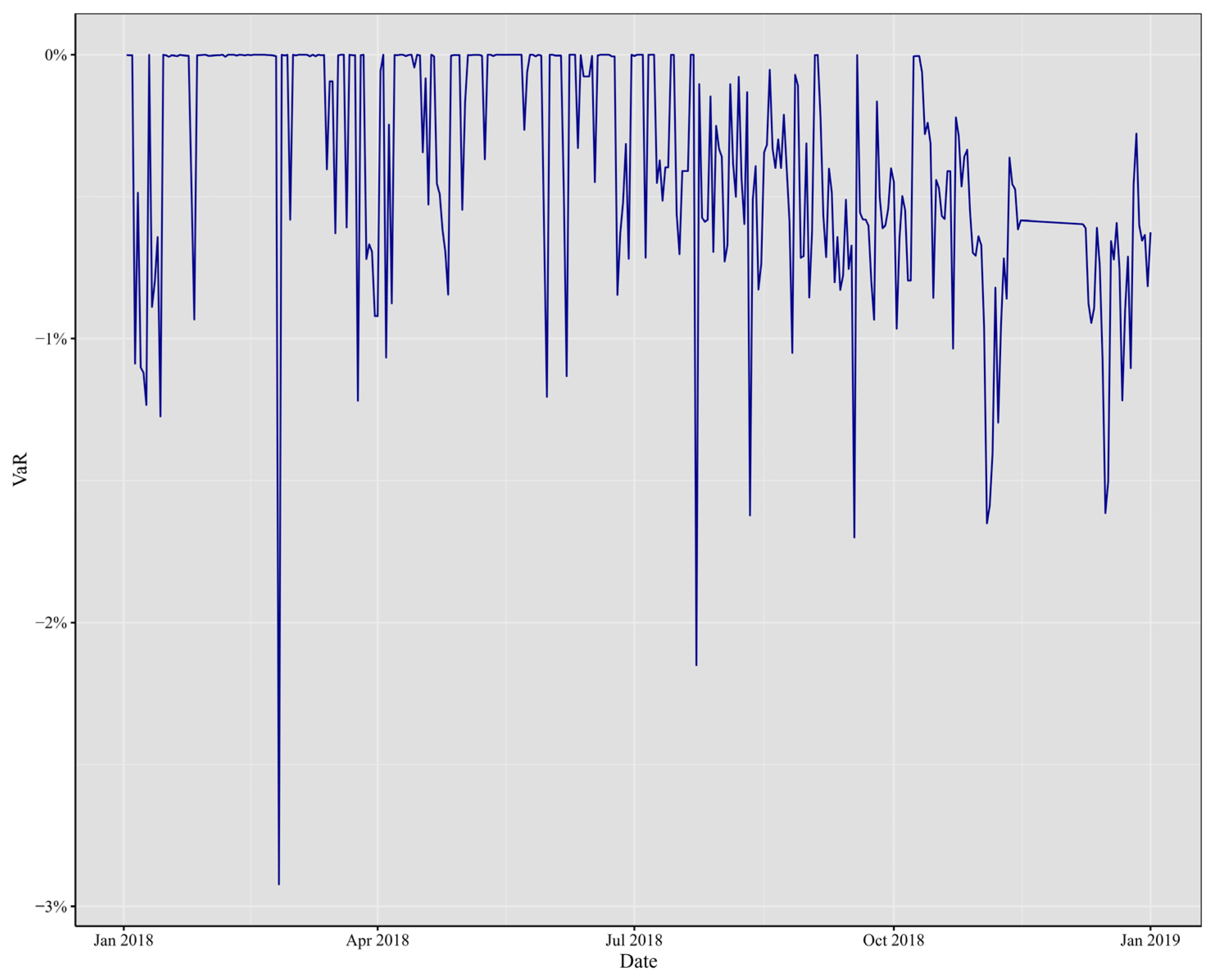
Fast forward to 2018, as depicted in
Figure 5, where minute VaR experienced significant fluctuations. January brought forth noteworthy developments: Ethereum soared to an all-time high, surpassing USD 1400, buoyed by the surging popularity of initial coin offerings (ICOs) on its platform. Meanwhile, Bitcoin underwent a correction after reaching a record high in late 2017, causing a market-wide downturn. The G20 summit in March became a focal point for discussions on cryptocurrencies and potential regulatory measures, injecting uncertainty and brief price fluctuations into the market. April marked the beginning of Bitcoin’s price stabilization after several months of correction. Ethereum grappled with scalability challenges, with the congestion caused by the blockchain game CryptoKitties taking center stage. In June, regulatory clarity emerged when the U.S. Securities and Exchange Commission (SEC) clarified that Bitcoin was not considered a security. However, August brought the SEC’s rejection of several proposed Bitcoin exchange-traded funds (ETFs), fostering market uncertainty and causing temporary price dips. Finally, by November, Ethereum’s price exhibited a significant decline, aligning with the broader trend in the cryptocurrency market.
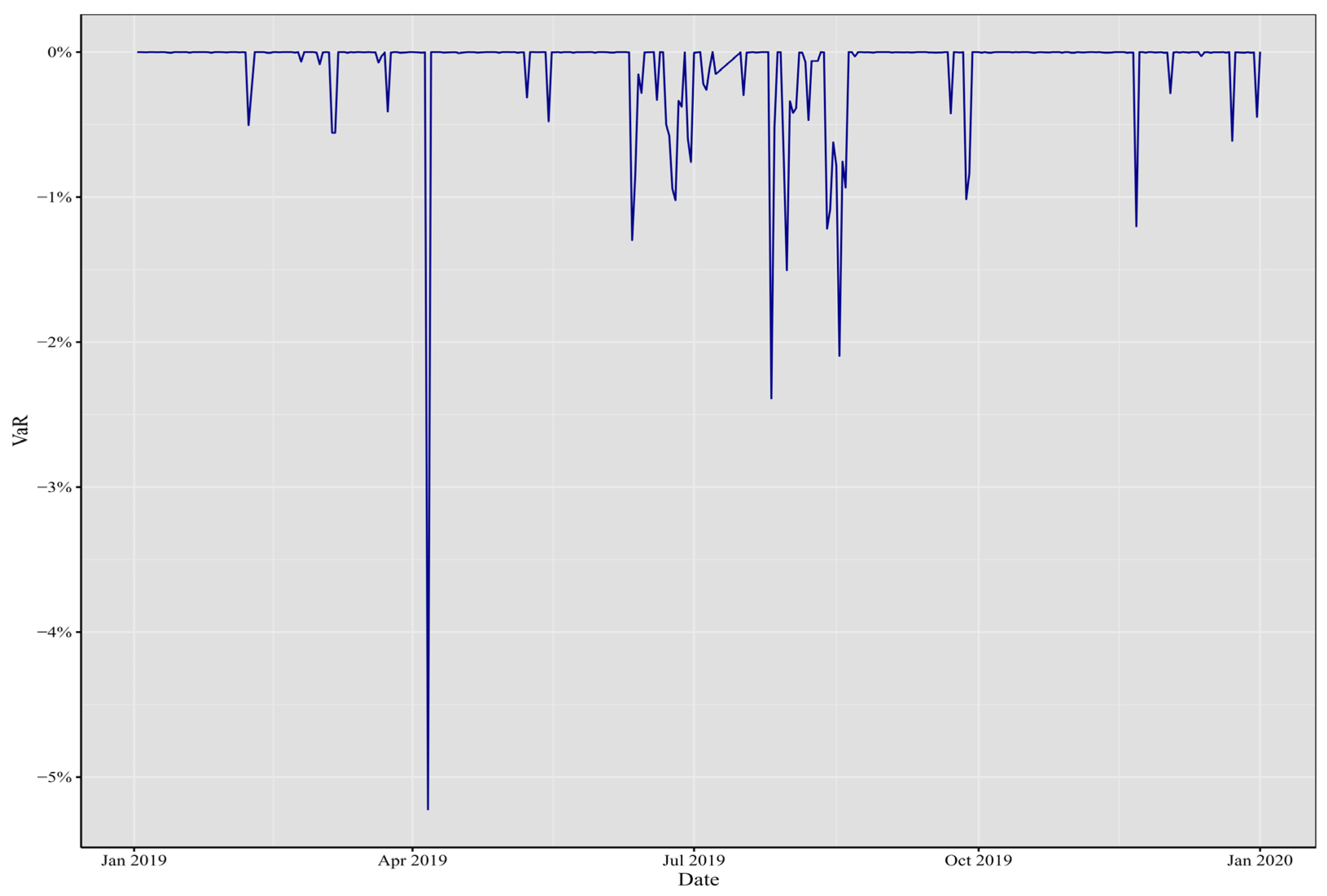
As we journeyed into 2019, depicted in
Figure 6, both Bitcoin and Ethereum experienced significant events and developments. Bitcoin commenced the year with anticipation of its halving in May, only to face a price decline in March during the global financial market crash triggered by the COVID-19 pandemic in 2020, depicted in
Figure 1. Ethereum, on the other hand, underwent a hard fork in February and announced Ethereum 2.0 in June, marking its transition to a proof-of-stake consensus mechanism. The decentralized finance (DeFi) sector continued to flourish on the Ethereum network throughout the year.
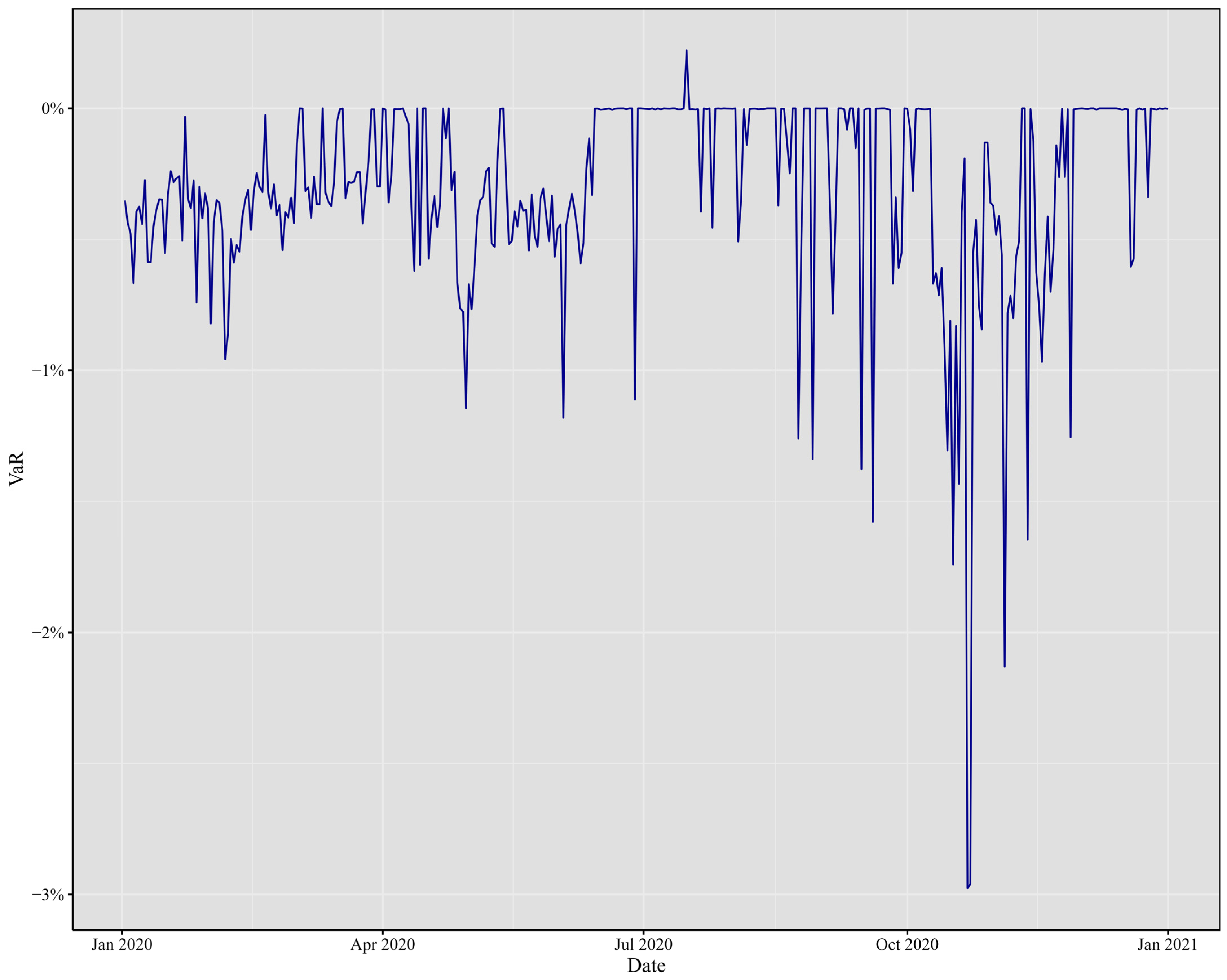
The year 2020, as illustrated in
Figure 7, was marked by Bitcoin’s rebound after the 2018 bear market. May brought the long-anticipated halving of Bitcoin, impacting its supply dynamics. In June, Facebook’s Libra project announcement triggered discussions on regulation. Ethereum implemented the Beacon Chain testnet as part of the Ethereum 2.0 upgrade in July. August witnessed a surge in institutional interest in Bitcoin, notably with MicroStrategy’s substantial investment.
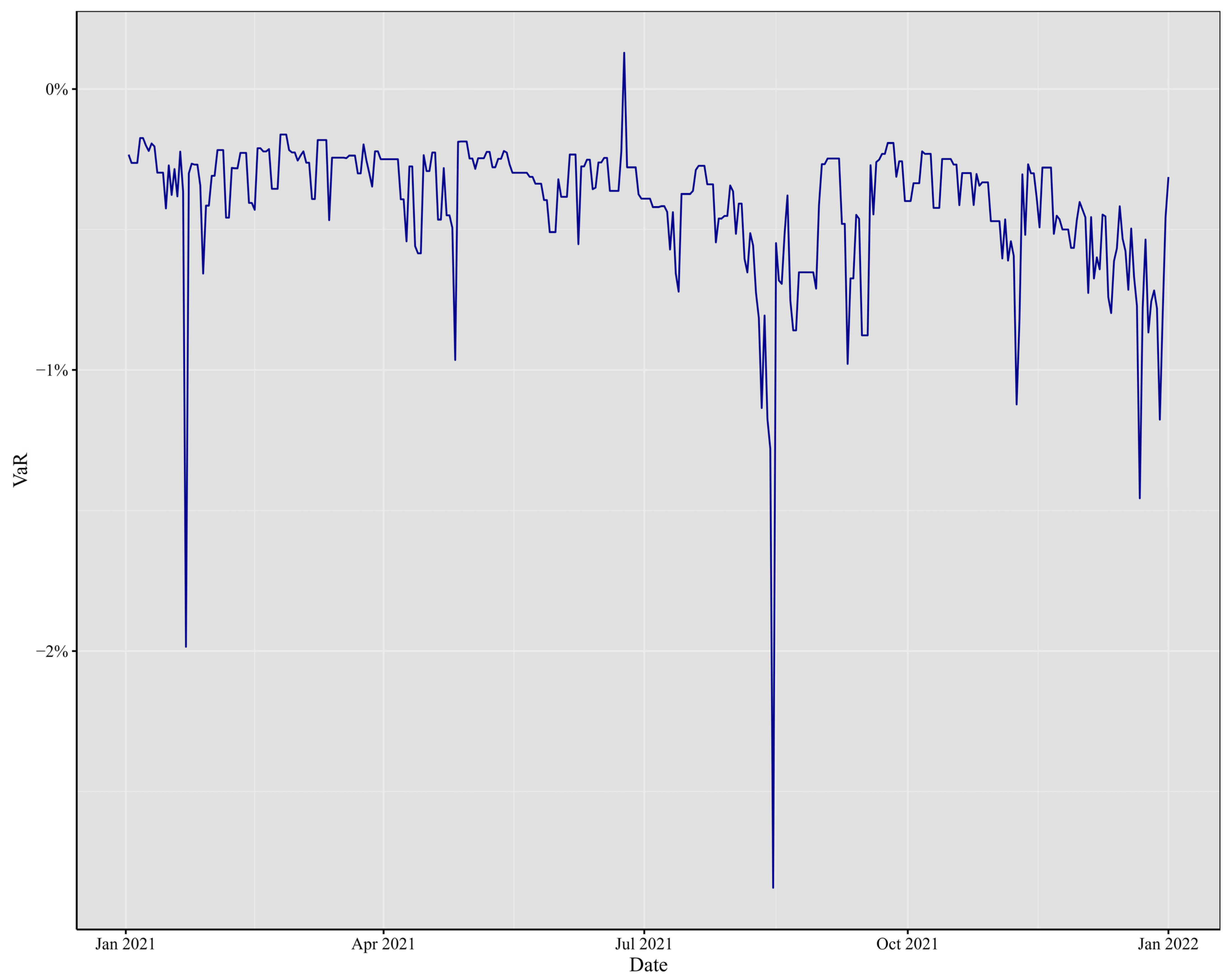
Turning to 2021, as depicted in
Figure 8, Bitcoin experienced a remarkable price surge, reaching new all-time highs, driven by institutional investments and positive sentiment. Tesla’s announcement of a significant Bitcoin investment in February further solidified Bitcoin’s mainstream acceptance. Ethereum’s price also soared in February. However, in May, Bitcoin underwent a correction due to environmental and regulatory concerns. In June, El Salvador adopted Bitcoin as legal tender, marking a groundbreaking moment for cryptocurrency adoption. Ethereum introduced key upgrades, including the Berlin hard fork in April, the EIP-1559 upgrade in August, and in November, aiming to enhance its efficiency and address fee-related issues.
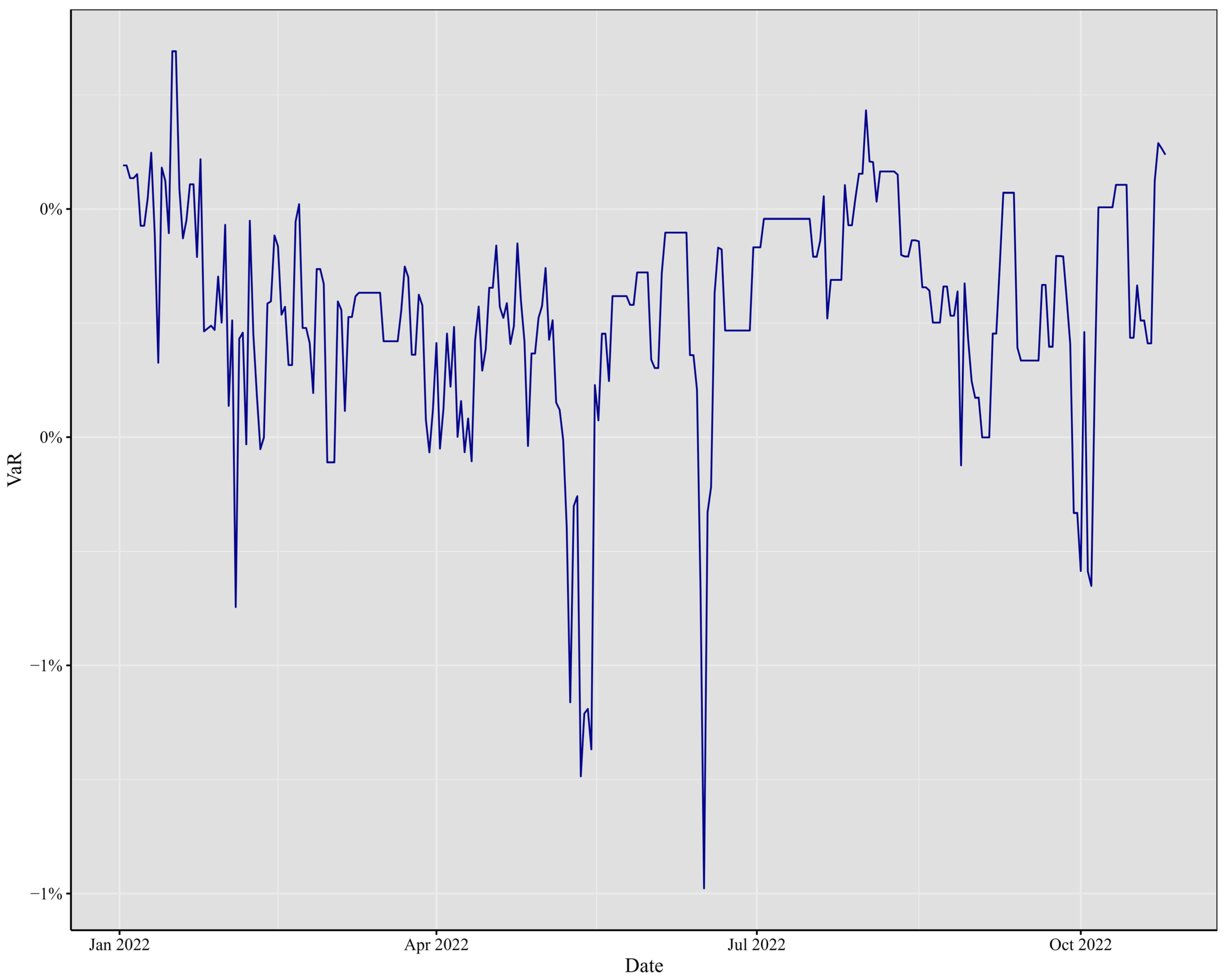
Finally, in 2022, as depicted in
Figure 9, the cryptocurrency industry played host to several significant events. February took center stage during the Super Bowl with the “Crypto Bowl,” where industry giants like Coinbase, FTX, Crypto.com, and eToro stepped forward to showcase their products to an estimated 200 million viewers. In May, turmoil ensued as Terra’s algorithmic stablecoin TerraUSD (UST) witnessed a wavering U.S. dollar peg, resulting in a substantial value decline. June witnessed a contagion effect as crypto lender Celsius froze operations due to “extreme market conditions,” while Voyager issued a notice of default to hedge fund Three Arrows Capital (3AC). Ethereum brightened the year in September with “The Merge” upgrade, making the network significantly more energy-efficient. However, October proved to be a bountiful month for crypto hackers, who managed to abscond with over USD 718 million from decentralized finance sites in a series of high-profile hacks, underscoring the security challenges inherent in the DeFi sector.
Throughout these years, the cryptocurrency world bore witness to remarkable transformations, from the surge in adoption and institutional investment to regulatory developments and technological upgrades, creating a vibrant and ever-evolving landscape for Bitcoin and Ethereum.
The VaR estimation for the equally weighted portfolio across different years reveals intriguing characteristics. Notably, despite the economic and financial turbulence experienced in various periods, the greatest volatility in VaR estimation occurs in 2017, rather than in 2020. This observation suggests that other factors beyond the pandemic played significant roles in shaping market volatility during these periods. Interestingly, in both 2022 and 2021, we observe the lowest volatility in VaR estimation, indicating a potential stabilization of the market following the peak of the crisis. Additionally, it is noteworthy that the corresponding volatilities of the years 2018, 2019, and 2020 are remarkably similar.
However, the mean values in 2020 and 2018 are three times higher than that of 2019, indicating differing levels of risk exposure across these years. This discrepancy in means, as a measure of central tendency, implies a need for higher capital requirements in 2018 and 2020 compared to 2019. Moreover, the year with the highest mean is 2017, indicating greater volatility in terms of VaR. Furthermore, it is observed that the VaR for 2021 and 2022 exhibits similar means but significantly lower volatility compared to 2017. These findings highlight the dynamic nature of cryptocurrency markets and the importance of understanding the underlying factors influencing risk across different time periods.
In terms of Value-at-Risk (VaR) computation, we derived it using the theoretical values of the 1% left tail of the marginal distribution for the portfolio. Several noteworthy phenomena emerged from the analysis. In 2020 and 2021, the one-minute VaR for a given day exhibited positive values, indicating that during these periods, the expected market behavior leaned heavily in favor of the participants. It is important to note that VaR values might not remain consistent day after day; however, the computation of this statistic revealed its non-stationary nature when applied to intraday data.
The observation is significant as it sheds light on why we obtained means that are almost zero in the VaR statistics presented in
Table 4. This observation is crucial because it reflects the behavior in the level of daily VaR constructed from minute-by-minute prices.
Figure 1, depicting the movements of Bitcoin and Ethereum, provides insight into this phenomenon. We can observe movements in different directions, contributing to the explanation of the near-zero means. However, it is noteworthy that Ethereum reflects higher volatility compared to Bitcoin. The construction of an equally weighted portfolio also contributes to this aspect of near-zero means. In conclusion, the behavior of Bitcoin and Ethereum prices, coupled with the construction of the portfolio, has led to this characteristic of the means.
To validate the practical applicability of these computations, a forward testing technique was employed. Using the previous day’s one-minute VaR as a benchmark, we monitored whether the returns fell below this threshold. A return breaching the VaR boundary was considered a failure. This evaluation was conducted for all 1440 min of each day, assessing whether they fell within the VaR limit or not. Finally, we calculated the mean of this Bernoulli distribution as a proxy for the probability of VaR accurately predicting the 99% threshold.
Figure 10,
Figure 11,
Figure 12,
Figure 13,
Figure 14 and
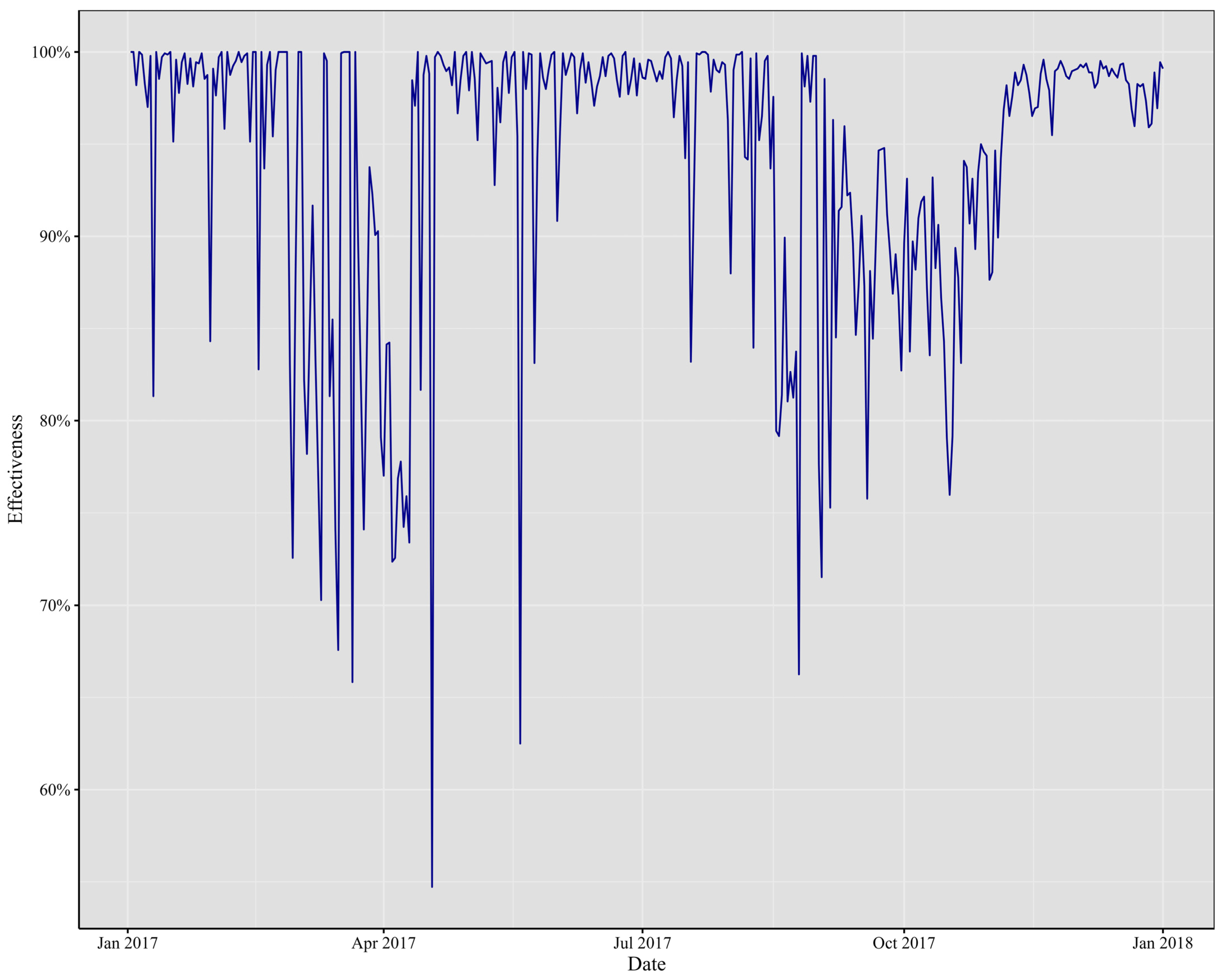
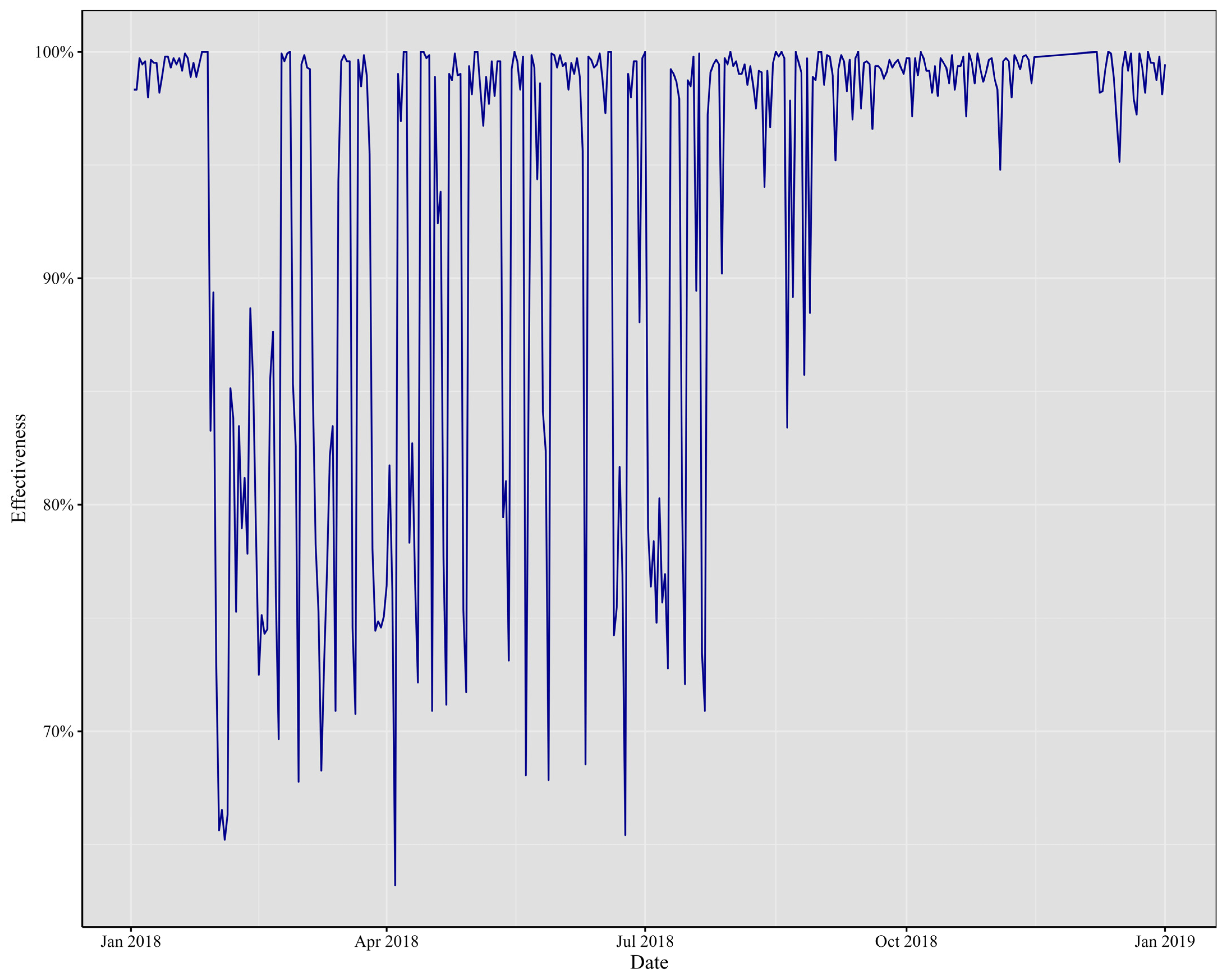
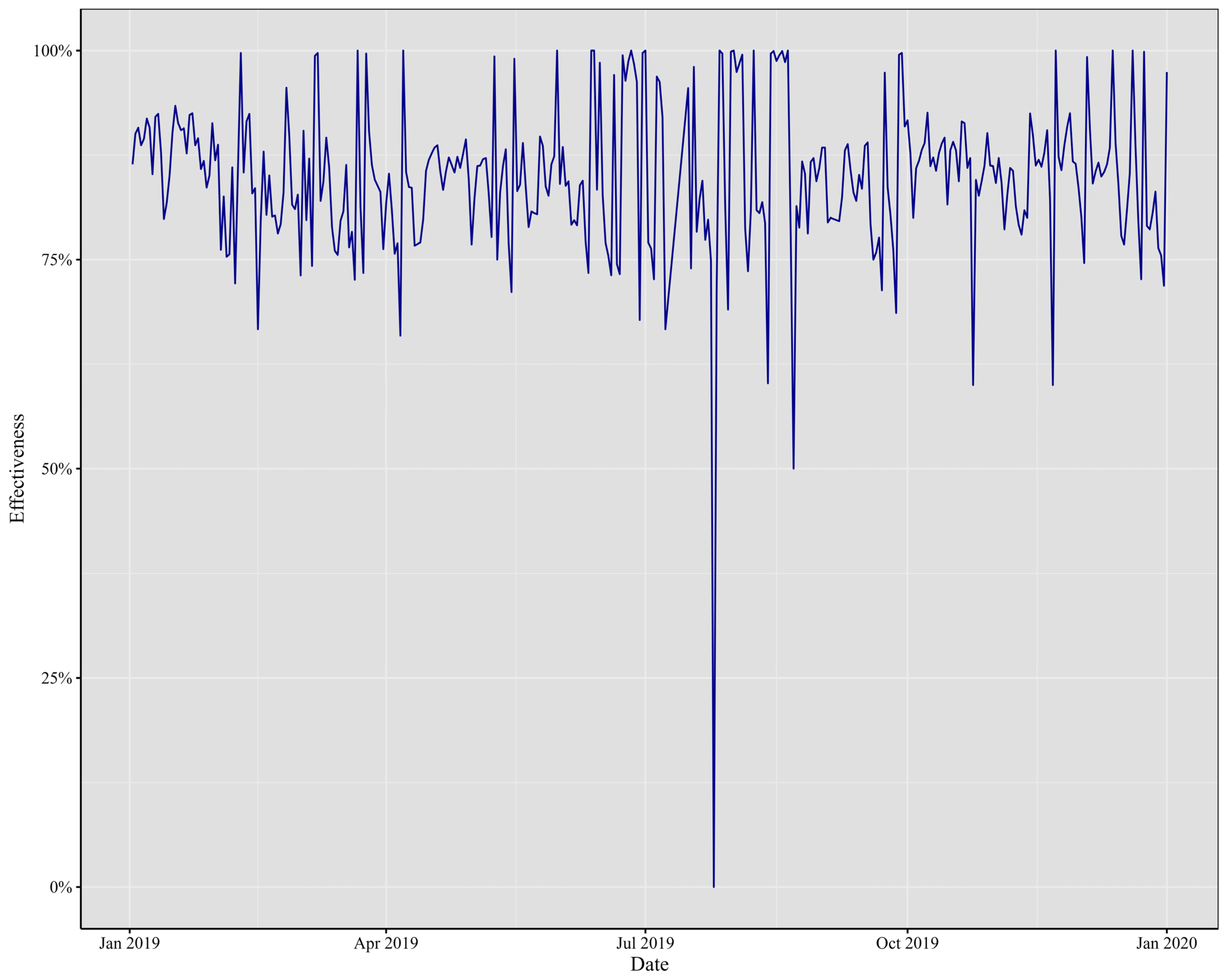
Figure 15 depict the daily effectiveness of this risk measurement.
Table 5 displays the performance metrics for the year 2017. We observed a high mean value of 0.9411, indicating the average daily returns of our portfolio. However, it is important to note that the minimum value recorded during this period was 0.5472. This variability in returns reflects the dynamic nature of our portfolio components. Notably, the minimum value occurred shortly after the beginning of April, highlighting a specific instance of lower performance within the observed timeframe.
In
Table 6, we present the performance metrics for the year 2018. Similar to 2017, the mean effectiveness for 2018 remains high, exceeding 90%. However, it is noteworthy that we observed a minimum value of 0.6319, which occurred very close to the beginning of April. This minimum value surpasses the lowest recorded value in 2017, indicating a different performance trend during this period.
In
Table 7, we analyze the data for the year 2019. Remarkably, only one day exhibits an extreme event, where the minimum VaR effectiveness approaches zero. However, for the majority of the year, we observe significantly higher effectiveness compared to both 2017 and 2018. This consistent pattern suggests improved risk management dynamics and highlights the evolving nature of cryptocurrency markets during this period.
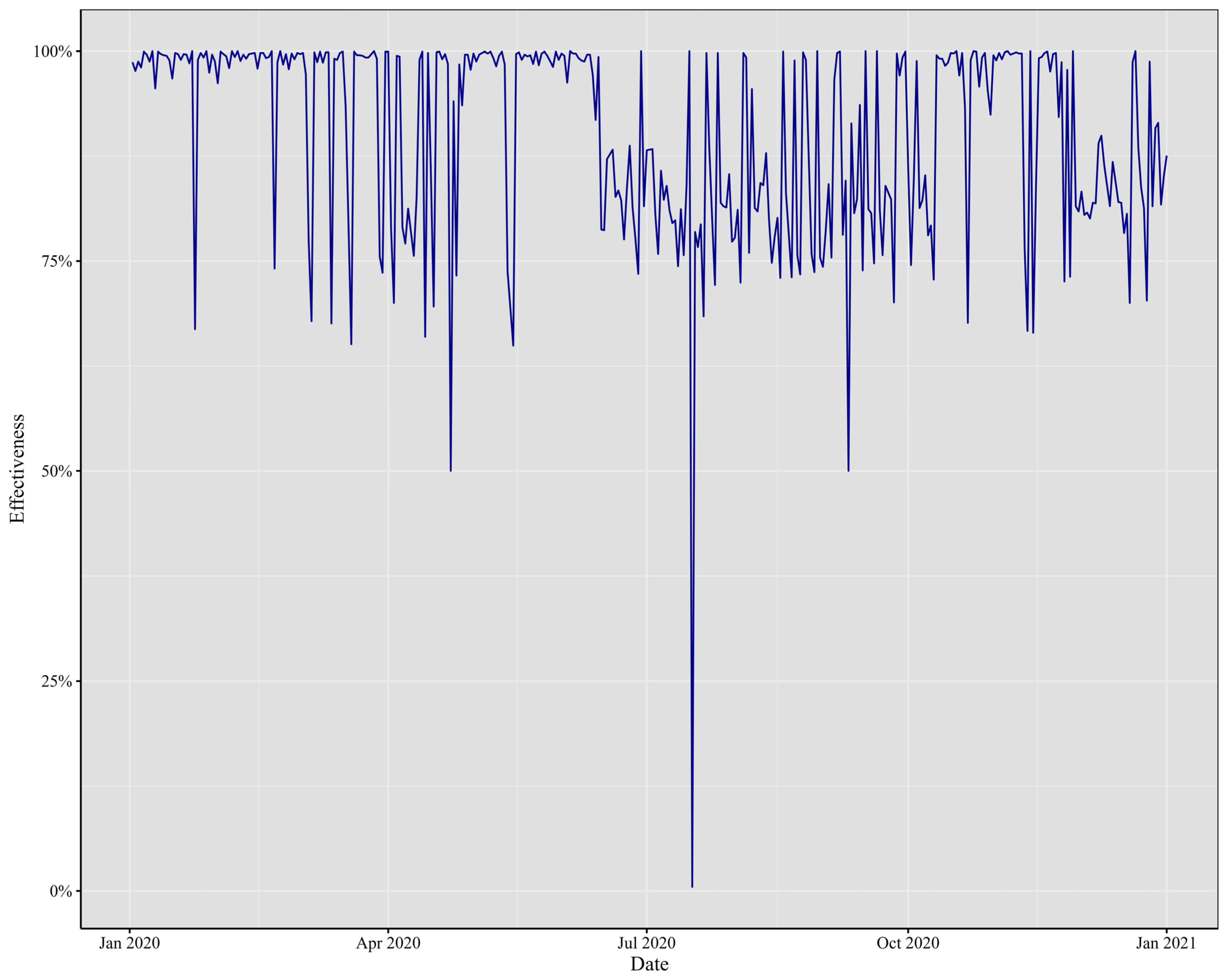
Table 8 illustrates the data for the year 2020. Similar to 2019, we observe a day with a minimum effectiveness close to zero, signifying an extreme event. Nonetheless, the effectiveness on the remaining days mirrors that of 2019, with a mean effectiveness exceeding 90%. This consistency underscores the robust risk management dynamics prevalent throughout the year, despite occasional extreme occurrences.
Table 9 presents the mean effectiveness of VaR for the year 2020, which stands remarkably high at 0.9827. This exceptional level underscores the overall robustness of the risk management framework during this period. However, it is noteworthy that there is one day with significantly lower effectiveness (0.0945), observed near the beginning of July. This outlier indicates an exceptional event where the effectiveness of VaR deviated from the norm, as illustrated in the graph.
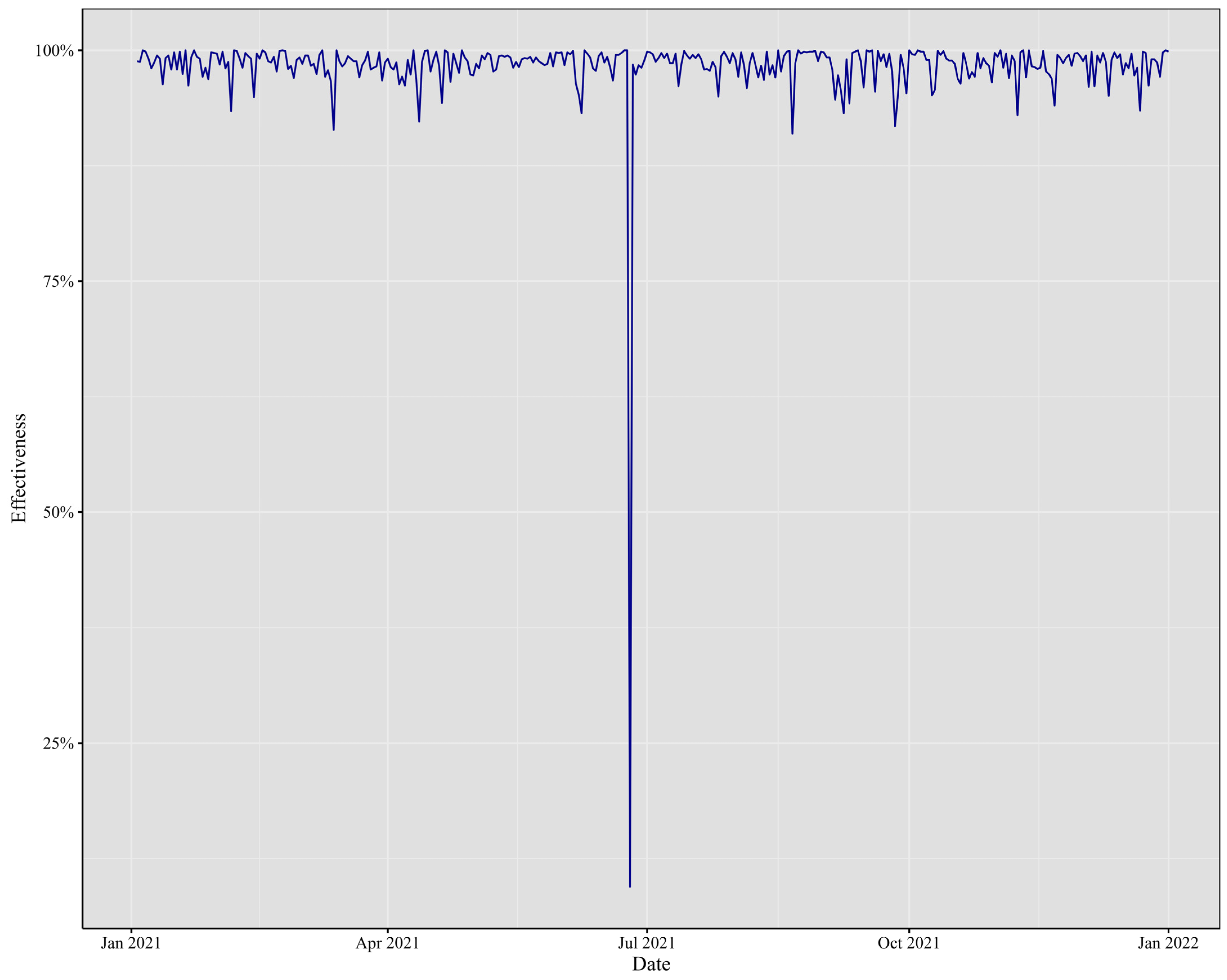
Table 10 highlights the observations for the year 2021. In contrast to previous years, we observed more variability in the estimation of VaR. Despite this variability, it is notable that the minimum effectiveness remained remarkably high at 0.9361. This finding suggests increased stability in our equally weighted portfolio concerning the estimation of VaR for the year 2021.
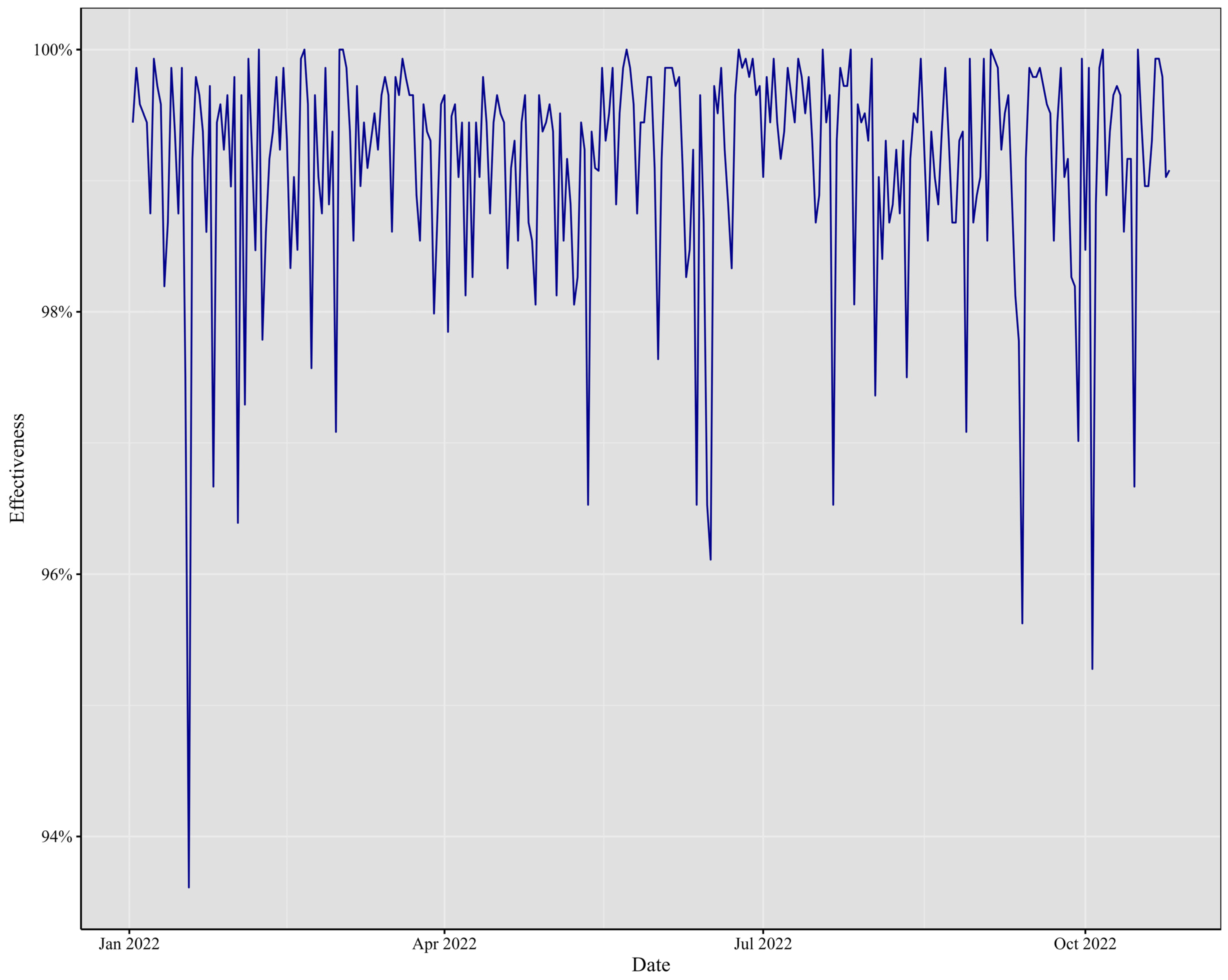
In summary, the VaR values across the years 2017, 2018, and 2019 demonstrated relatively lower effectiveness when compared to the subsequent years of 2021 and 2022. Notably, in the latter two years, the effectiveness of VaR exceeded the 95% threshold, showcasing robust risk assessment capabilities, with only one isolated instance of deviation noted in 2021. Conversely, the observed behavior in the preceding years exhibited a consistent pattern of performance.
Across the cryptocurrency landscape from 2017 to 2022, a sequence of impactful events unfolded. Noteworthy rallies, regulatory developments, and technological upgrades marked each year. Interestingly, 2019 exhibited a smaller mean effectiveness, hinting at heightened variability in the minute Value-at-Risk (VaR) values. Despite this, the majority of the mean values surpassed 90%, underscoring the enduring impact of these events. In 2021 and 2022, a distinct trend emerges. The theoretical VaR at the 99% confidence level closely aligns with the empirical test results, hinting at an evolving behavior in both the daily and intraday cryptocurrency data. This observation signifies the dynamic nature of the cryptocurrency market, where events not only influence daily trends but also shape intraday movements.
With an increasing number of financial institutions incorporating high-frequency trading into their investment strategies, models like the one presented here exhibit sufficient power and flexibility to adapt to the volatile nature of these assets.
5. Conclusions
This paper has introduced an intraday risk management procedure, employing one-minute interval data, for the two major cryptocurrencies. By computing VaR on a day-by-day basis, a one-minute 99% confidence level benchmark was established. This benchmark served as a reference point for evaluating the returns on the following day, with success defined as the empirical value remaining within the VaR.
The results demonstrate the effectiveness of the Multivariate Normal Inverse Gaussian (NIG) distribution in capturing the volatile behavior of assets like cryptocurrencies. Intraday data exhibit even more pronounced stylized facts than daily frequency data, making the ability to model them a competitive advantage in risk management. Moreover, from a computational standpoint, implementing these models is relatively cost-effective compared to the Generalized Hyperbolic Distribution.
This study also highlights potential areas for future research. Specifically, it raises questions about the extreme behavior observed on certain dates when the algorithm failed to converge. Exploring heavy-tail distributions and extreme value theory may provide solutions to modeling such episodes and identifying intraday bubble events. The detection of critical dates with extreme behavior is a significant result that warrants further investigation.
Lastly, the successful adjustment of the model for 2021 and 2022 suggests that this approach is promising for diversification techniques. Incorporating diverse assets may be the solution for enhancing the diversification of cryptocurrency portfolios. However, challenges related to data manipulation and standardization could restrict the model’s application. Nevertheless, the evidence from this research supports the consideration of this technique by both practitioners and academics.
In addition to the findings presented in this study, there are opportunities for further research that can enhance our understanding of cryptocurrency risk management. One such avenue involves exploring how different portfolio compositions affect Value-at-Risk (VaR) in cryptocurrency investment.
While our paper utilized an equally weighted portfolio, we acknowledge the importance of examining alternative portfolio strategies to better understand their implications for risk assessment. We decided to opt for equal weights due to the challenges associated with achieving diversification in cryptocurrency markets. However, future research could investigate how employing different weighting schemes affects VaR behavior.
With the advancement of technology, particularly in the realm of machine learning, researchers can explore more sophisticated statistical models for VaR estimation and prediction. Recently, solutions using machine learning models have emerged, involving training algorithms to forecast variables. Given the abundance of data available in cryptocurrency markets, researchers can estimate VaR for a portion of the sample and predict for the rest of the timeline.
By conducting analysis using various portfolio allocation methods, including, but not limited to, equally weighted portfolios, and incorporating machine learning techniques for VaR estimation and prediction, researchers can gain insights into how different compositions and modeling approaches influence risk management outcomes. This approach would allow for a more comprehensive evaluation of portfolio diversification strategies and their effectiveness in mitigating risk in cryptocurrency investment.
Through such research endeavors, the researchers aim to contribute to the ongoing discourse on cryptocurrency risk management practices and provide valuable insights for investors and policymakers navigating this rapidly evolving landscape.


 ,
, 


