
The Regime-Switching Structural Default Risk Model
1
Department of Accounting & Finance, Faculty of Economics & Management, University of Cyprus, P.O. Box 420537, CY-1678 Nicosia, Cyprus
2
Accounting and Finance Division, Alliance MBS, University of Manchester, Manchester M13 9PL, UK
*
Author to whom correspondence should be addressed.
Risks 2024, 12(3), 48; https://doi.org/10.3390/risks12030048
Submission received: 12 January 2024
/
Revised: 16 February 2024
/
Accepted: 26 February 2024
/
Published: 4 March 2024
(This article belongs to the Special Issue Risks Journal: A Decade of Advancing Knowledge and Shaping the Future)
Abstract
:We develop the regime-switching default risk (RSDR) model as a generalization of Merton’s default risk (MDR) model. The RSDR model supports an expanded range of asset probability density functions. First, we show using simulation that the RSDR model incorporates sudden changes in asset values faster than the MDR model. Second, we empirically implement the RSDR, MDR and an extension of the MDR model with changes in drift parameters, using maximum likelihood estimation. Focusing on the period before and after corporate rating downgrades used primarily for investment advice, we find that the RSDR model uses changes in equity mean returns and volatility to produce higher estimated default probabilities, faster, than both benchmark models.
1. Introduction
Increased equity volatility and negative abnormal stock returns have been shown to precede downgrades in corporate bond ratings (Holthausen and Leftwich 1986; Hand et al. 1992; Goh and Ederington 1993, 1999; Vassalou and Xing 2005). Structural models of default risk use equity price dynamics to infer the distribution of the unobserved value of assets and consequently an estimate of the default probability. Changes in equity mean returns and volatility can be incorporated into asset distribution dynamics if option pricing models can accommodate such features as jumps, bimodality, excess kurtosis and skewness because they will in general transform into heavier tails and hence more representative estimates of default probabilities. Since the combination of increased volatility and negative abnormal returns precedes downgrades in bond ratings (Milidonis and Wang 2007) but also in sovereign debt ratings (Michaelides et al. 2015, 2019), we expect that the estimated distribution of assets will also be affected.
In this paper, we develop an extension of Merton’s (1974) default risk (MDR) model that can accommodate such flexibility in the estimated asset distribution in a regime-switching environment. The application of regime-switching models to the prediction of default risk is appealing for several reasons: regime-switching models allow the construction of a firm-specific (log) asset return distribution with non-normality features; they produce heavier tails in asset return distributions than competing models, and hence their estimated default probabilities are more accurate; they accommodate both sudden changes and extended periods of abnormal trends in the mean and volatility of asset returns by classifying them in separate regimes; they identify the exact time and duration of new regimes.
We contrast both the cross-sectional and time-series properties of the regime-switching default risk (RSDR) model with those of the MDR model, for both simulated and real data. Using simulated data, we show that the RSDR model is more responsive to changes in default risk than the MDR. This responsiveness is more evident in cases of increasing default risk because the MDR model assumes a more rigid distribution for asset returns than the RSDR model.
Our next step is to conduct an empirical exercise of the RSDR model vs. the MDR model to test their responsiveness to market-implied changes in default risk. In addition, we compare the properties of the RSDR model with a variation of the MDR model with jumps (MDRJ), which resembles the models of Zhou (2001b) and Cremers et al. (2008).1 Because of the asymmetry in market reactions to downgrades and upgrades (e.g., Holthausen and Leftwich 1986; Hand et al. 1992; Ederington and Goh 1998), we focus our empirical analysis on a sample of rating downgrades. We use rating downgrades by Egan Jones Ratings (EJR), which uses publicly available information to produce its ratings and has also been found to publish timelier ratings than its major competitors such as Standard and Poor’s (S&P) and Moody’s (Johnson 2004; Beaver et al. 2006). Beaver et al. (2006) highlight that over the period 1997–2002, EJR ratings were not certified by the Securities and Exchange Commission (i.e., EJR announcements did not carry a regulatory weight), and they were used only for investment advice. Therefore, we use downgrades by EJR as a proxy for the arrival of market-implied information related to increasing default risk.
We estimate daily probabilities of default on a rolling-window basis using the MDR, MDRJ and RSDR models for the one-year period before and after the sample of EJR’s downgrades. Consistent with the literature, we find that over this period, equity (hence asset) log-returns experience changes in both their mean and volatility. In contrast to the MDR model, the RSDR model can reflect such non-normality in equity (asset) log-returns in default probabilities. We find that over the fifty days preceding downgrades, the RSDR model produces higher awareness of the imminent increase in default risk. We measure this as the difference in the default probabilities from the two models, which increases before, peaks at and decreases after the downgrade. When we compare the RSDR and MDRJ models, we find that the RSDR model is still more responsive than the MDRJ model for the period leading to a downgrade.
The rest of the paper is organized as follows: In Section 2, we review the literature on structural default risk and regime-switching models. In Section 3, we introduce the RSDR model and describe its estimation using the transformed maximum likelihood approach. In Section 4, we present applications of the RSDR and MDR models on simulated and real data. In Section 5, we discuss the flexibility of the RSDR model, estimate a variation that resembles the MDR model with jumps (MDRJ) and compare it with the RSDR model. Section 6 concludes.
2. Structural Default Risk Models and Structural Breaks
The seminal work of Black and Scholes (1973) and Merton (1974) initiated a large strand of literature on structural models of default.2 Since then, numerous papers relaxed many of the original assumptions used in the MDR model: stochastic vs. constant interest rate (Shimko et al. 1993; Acharya and Carpenter 2002), seniority of debt (Black and Cox 1976), default correlation (Zhou 2001a) and the default boundary which is either set exogenously (Longstaff and Schwartz 1995) or chosen endogenously by managers to maximize shareholder value (Leland 1994; Leland and Toft 1996; Huang and Huang 2012). We use the MDR model with a constant interest rate and an exogenous default boundary, as the first benchmark for our analysis.
On the distribution of the estimated value of assets, Zhou (2001b) introduces jumps in the underlying diffusion process of the MDR model. Cremers et al. (2008) also use a jump–diffusion model. Even though such a model can capture sudden jumps in asset values and can reduce the underestimation of default probabilities (Leland 1994), a jump is only one way to incorporate new information in the markets. Another way is the gradual, incremental leaking of information, which will likely affect the mean and volatility of log-asset returns. Hull and White (1987, 1988) find that option Vega can be used as a good approximation of stochastic volatility models for European options. However, Vega works well only for small changes in volatility after an event, not for large changes such as stock market crashes or regime changes (Avellaneda et al. 1995). In a jump–diffusion model, structural changes in volatility might be interpreted as a series of small jumps, therefore overestimating the frequency and underestimating the average magnitude of jumps.
Comparison of Regime-Switching Models with Competing Models
The concept of Markov regime-switching models for use in econometric applications was first described by Quandt (1958), and Goldfeld and Quandt (1973). Regime-switching models are characterized by the assumption that the transition probability between regimes on the observation is dependent only on the state that the system was in on the previous, , observation. Goldfeld and Quandt derive a maximum likelihood estimate of the transition probabilities, linear model coefficients and innovation variances. Hamilton (1989) further improves regime-switching models by developing a full-sample smoother framework, which uses all measurement data (rather than just historical data) to compute the conditional probability estimates. An overview of the likelihood maximization techniques and specific guidance for the transition probabilities is given by Hamilton and Susmel (1994).
We argue that the regime-switching models are more appropriate than previous models (i.e., jump–diffusion models; “long-memory” autoregressive-type models) in capturing asset return dynamics in the following ways: First, the unobserved Markov chain can identify not only isolated jumps in log-asset returns (i.e., similar to jump–diffusion models), but also jumps in return volatility, or a combination of both. Second, returns with structurally different characteristics are isolated into separate regimes of varying mean, volatility and/or duration. Third, the memoryless property of the Markov chain reduces the possibility of the long-memory feature of autoregressive-type models, which “contaminates” future forecasts of estimated probabilities of default with old and potentially less useful information. Fourth, the overall return distribution becomes a weighted average of the time spent in each regime without spillover effects from one regime to another.
Our argument in favor of regime-switching models is supported by several empirical studies in economics and finance (Litterman et al. 1991; Gray 1996; Ang and Bekaert 2002a, 2002b; Poon and Granger 2003; Kalimipalli and Susmel 2004).
3. The Regime-Switching Default Risk (RSDR) Model and Its Estimation
3.1. Lognormal Regime-Switching Asset Price Model
We let be the value of assets of the firm on day and the log-asset return In contrast to the MDR model which assumes that asset log-returns ( are distributed normally with a constant drift () and variance (), we assume that asset log-returns switch between state-dependent normal distributions according to a hidden Markov chain.
We assume that the asset process is governed by two states (regimes); hence, the switching behavior of assets is captured by the following transition probabilities: , where is state on day , and and take values in the range . We assume that the transition probabilities are constant through time, unobservable and constrained:
Conditional on being in state on day , asset log-returns follow a normal distribution with constant drift and volatility:
Hence, for the two-regime model, the distribution of assets can be characterized by six parameters: .
We assume that the market value of equity of a firm on day , , equals the value of the European call option that shareholders have on the assets of the firm. To develop a self-contained and observable structural model for default risk based on a regime-switching model for asset returns, we need to link the value of unobserved assets of the firm to the observed value of equity. Therefore, we use the option price equation under a regime-switching asset process, which has been developed in the asset pricing literature (Naik 1993; Hardy 2001; Boyle and Draviam 2007).
3.2. Estimation
There are several methods for estimating structural default risk models with real data (Li and Wong 2008). The “volatility-restriction” method (Ronn and Verma 1986) estimates the parameters of the asset-return distribution by using an approximation of log-asset volatility and the average return from the estimated value of log-assets. The estimates of the value, drift and volatility of assets are used to calculate the probability that assets will be less than the value of debt at the one-year horizon (Jones et al. 1984; Ronn and Verma 1986, 1989; Ogden 1987; Lyden and Saraniti 2001; Huang and Huang 2012; Vassalou and Xing 2004).
A more recent method that is superior to the “volatility-restriction” method is the maximum likelihood estimation (MLE) approach introduced by Duan (1994, 2000) and used widely in the literature (Duan and Yu 1994; Duan and Simonato 2002; Ericsson and Reneby 2004, 2005; Lehar 2005; Li and Wong 2008; Duan and Yeh 2010, among others). The MLE approach estimates the parameters of the log-asset return distribution directly from equity observations.
We use the MLE approach to estimate the RSDR model and the benchmark MDR model. The MLE approach requires five steps. First, we choose a structural default risk model (e.g., RSDR or MDR). Second, we derive the equity option pricing equation. Third, we derive the equity likelihood function as a function of the (unobserved) asset values, assuming a one-to-one transformation between equity and asset values. The equity likelihood function is then a function of the parameters of the asset distribution that we estimate. Fourth, we maximize the likelihood function subject to the constraint that the option pricing equation holds for each of the time-series () observations in the sample. Fifth, we estimate the value of assets by solving the European option pricing equation (constraint) using the estimated parameters of the asset distribution and the observed value of equity. We set up the mathematical framework for estimating the less complicated MDR model (Appendix A) and then follow the same process to estimate the RSDR model as explained below.
To implement the RSDR model (second step above), we follow the rationale of Hardy (2001) for the option-pricing equation under regime switching. To estimate the six asset parameters, , of the RSDR model, we need to derive an expression for the likelihood of , conditioned on :
We can obtain this expression if the probability of being in either regime is known for each observation . Hamilton (1989) develops a method to estimate the parameters of such a model by assuming that the probability of being in a regime at some future time is dependent only on the current regime. To estimate these probabilities, we use a variation of Hamilton’s (1989) recursive filter (Section 3.5 and Appendix B), which updates the joint conditional probability to give . This filter is also used to estimate the transition probability matrix. Then, we use the downhill simplex method (Nelder and Mead 1965; explained in detail by Vetterling et al. 2002) to maximize the likelihood function and obtain .
Given , we then estimate the probability that the asset value will be less than the value of debt at the one-year horizon, using the regime-switching probability density function. Following Vassalou and Xing (2004), we recognize that since this estimated probability might not reflect real default probabilities in the long term, we name this estimated probability the regime-switching default likelihood indicator (RSDLI). Similarly, we use MDLI for the default likelihood indicator from the MDR model.
3.3. Sojourn Probability Function
Both the regime-switching European option pricing model and propagation equations for the asset probability density function needed to produce the RSDLI require that we compute a “sojourn probability function”.3 Estimating the sojourn probability function is important because it serves as an index (ranging from 0 and 1 on a continuous scale) that classifies the underlying asset between the two regimes.
We follow Hardy (2001) in denoting the total number of days that the process spends in regime 1 as , where can take values from to . denotes the probability that the total number of days the process spends in regime is equal to . Next, we use to represent the total number of days spent in regime 1, but in the time period . The probability function of , , is a key component of the RSDR model (Section 3.4); hence, we describe its estimation in detail in the next paragraphs.
We use to define the probability of the number of days spent in regime 1 at time being , conditional on where the process is on the previous day. To illustrate this, consider the process when The probability that, starting on day , no days are spent in regime 1, given that the process is in regime 1 in the previous time period (i.e., ), is denoted by Hence, this is the same as the transition probability from regime 1 at time () to regime 2 at time ):
Similarly, we define the rest of the transition probabilities, which remain constant throughout all time periods in our model:
Having defined what happens in the last time step of our estimation (i.e., when ), we can now work in reverse order (from to ) to compute the probability function of , , in the following manner:
The rationale is that as soon as the process completes the transition at time , it will enter either regime 1 or regime 2, with probability or , respectively. This would imply that, if the process is in regime 1 at time , then only () days have to be spent in regime 1 in the period [ Similarly, if the process is in regime 2 at time , then days have to be spent in regime 1 in the period [. This approach allows us to estimate and , that is, the conditional probabilities of on the two regimes.
Assuming constant transition probabilities, then the stationary (unconditional) probabilities for regimes 1 and 2 are as follows:
Therefore, the unconditional probability function can be estimated as follows (Hardy 2001):
3.4. Asset Values
Next, we compute asset values from the observed equity values and the European option pricing equation. For the MDR model, there is a unique transformation from assets onto equity values through the equation of the European call option. Regime-switching models allow the mean and volatility parameters of the asset evolution process to change instantaneously; therefore, the market is incomplete, and the Q measure is not uniquely determined. We assume that the RSDR model captures idiosyncratic and not economy-wide jumps. Specifically, we adopt the framework consistent with option pricing models under regime switching developed in the asset pricing literature (Bollen 1998; Hardy 2001; Boyle and Draviam 2007; Siu et al. 2008) to create a unique link between the risk-neutral and risk-adjusted measure; that is, the Markovian transition probabilities do not change with the change of measure. Therefore, we substitute the regime-specific log-means with , where is the risk-free rate and is the variance of log-assets in regime .4 Hence, we can use the regime-switching option pricing equation to “back out” the value of assets as they are now uniquely mapped onto equity values.
Asset values are both a function of the unknown volatility parameters and a function of the sojourn probability function, which is in turn a function of the unknown regime transition probabilities. Duan (1994) shows that the maximum likelihood estimates of these parameters converge asymptotically and can be used in the pricing equation. The value of the regime-switching call option (equity), , on the value of assets of the firm, , with a default boundary (liabilities), , is
where
and and is the standard cumulative normal probability function.
We use the regime-switching option pricing equation to estimate the value of assets from observed equity observations. A necessary step in this estimation is the equation for the option delta. The option delta is in turn dependent on because the option value under regime switching is approximately equal to the expected value of the individual formulae, , if the length of time spent in each regime is known in advance:
In this setting, is the European call option pricing equation with its volatility and its option delta,, dependent on :
Differentiating Equation (11) yields the regime-switching option delta:
3.5. Hamilton Filter Modification
The next step in deriving the log-likelihood value is to modify Hamilton’s (1989) filter (Appendix B). Given the estimated value of assets from equity observations, , and the option delta, (Equation (16)), we then modify the likelihood function, (Equation (A18)), in the recursive filter with Equation (17). For the RSDR model, we follow the same steps as in the case of the likelihood function for equity measurements in the case of MDR (Appendix A, Equation (A8)) to derive the likelihood of each equity measurement conditional on each regime on observation for the RSDR model:
We can now work through Equations (A7)–(A10) in Appendix A to maximize the log-likelihood with respect to subject to the constraint that the regime-switching option pricing equation holds for all observations in the sample5:
3.6. Forecasting of Return Probability Density Function ()
Because we compute the sojourn probability function, , as part of the model estimation process, the mean and standard deviation of log-asset returns are dependent on and follow
respectively. We use these equations to forecast asset returns periods ahead by using the unconditional probability density function for the asset return process at time , defined at a random point :
where is the density function for a standard normal distribution and is the value of assets at time , where is the last asset observation in the sample. We then compute the regime-switching default likelihood indicator, RSDLI, as the probability that will be less than at the one-year horizon.
4. RSDR’s Significance and Applications
4.1. Significance of Model
The economic significance of the RSDR model is reflected in the cross-section of estimated default probabilities. Kealhofer (2003) finds that the MDR model can produce misleading default likelihood indicators. For example, when the distance to default (DD) equals 4 (the expected value of assets is four standard deviations away from the default boundary at the one-year horizon, assuming a normal distribution for the log-asset returns), the implied default probability is virtually zero, which in turn implies a rating of “AAA”. However, there is a problem with transforming a DD of 4 into a “AAA” rating, since mapping the same DD with Moody’s proprietary empirical default distribution produces a default probability of 0.5% (Kealhofer 2003). This probability is the equivalent default probability of a non-investment-grade bond.
There is also economic value in the time-series characteristics of the RSDR model. Structural changes in equity, and consequently in assets, are smoothed out in the MDR model. Smoothing asset values means that periods of high (low) volatility in log-returns are underestimated (overestimated) by the assumption of constant volatility. The RSDR model helps remedy the underestimation of default probabilities by the MDR model. The more accommodating regime-switching distribution of the RSDR model produces a distribution tailored to the evolution of each firm’s asset values. In the next two sections, we conduct a simulation study (Section 4.2) and an empirical exercise (Section 4.3) to compare the properties of the RSDR model to those of the MDR model.
4.2. Simulation Results
We simulate equity trajectories where both models are expected to perform equally well (i.e., the underlying equity process is a geometric Brownian motion; Figure 1). Then, we simulate equity trajectories that correlate with potential increases and decreases in default probabilities (Figure 2 and Figure 3, respectively). We test the MDR and RSDR models on these simulated paths as explained below.
To estimate the default likelihood indicator using both models at the one-year (252 trading day) horizon, we estimate parameters using data from the previous year. For example, to estimate the probability that the company will default at days, we must first estimate each model’s parameters using data over the period to . Inputs to both the MDR and RSDR models are the market value of equity, the firm’s default boundary and the market risk-free rate. We set the market value of equity (MVE) of the firm on day at USD 50, the default boundary at USD 200 and the risk-free rate and dividends at zero.
In the first case we examine (Figure 1), we test the differences in the two models when there are no major changes in the underlying equity process. In this scenario, we expect that both models will produce similar default probabilities. Since the RSDR model includes two regimes by construction, we expect that the stationary probabilities between the two regimes will be either almost equal (around 50%) or very close to their upper and lower bounds (i.e., and will be equal to 0 and 1, respectively, or vice versa). In the case of similar stationary probabilities, we expect the mean and volatility parameters of the RSDR model to produce an upper and lower range for the parameters of the MDR model.6 We choose to simulate the MVE on a daily basis according to a lognormal distribution with a daily mean of and volatility of .7 For convenience, the default boundary (USD 200) and risk-free rate (0%) remain constant over the entire period.
In Figure 1 (Panels A and B), we show the estimated default likelihood indicators, mean parameters, and volatility parameters of the MDR and RSDR models for two scenarios of the simulated lognormal equity process. The vertical axis of the top left chart shows the evolution of the MVE. In the top right chart, we show the MDLI compared to the RSDLI from day 252 to 312. In the bottom left chart, we show the estimated volatilities of MDR (MDR_σA) and RSDR (RSDR_σ1 and RSDR_σ2), as well as the stationary probability that the system is in state 2 over the 252 sample days, RSDR_π2. For example, when the estimated RSDR_π2 equals 90%, this means that the asset return process lies in regime 2 for 90% of the 312 days and in regime 1 for 10%. In the bottom right chart, we show the estimated means of MDR (MDR_μA) and RSDR (RSDR_μ1 and RSDR_μ2). At any point in time, our models are estimated using 252 daily equity, debt and interest rate observations. Every time we add a new observation to our sample (i.e., the models are estimated on a daily basis using the 252 most recent observations), we remove the oldest observation from the sample and re-estimate both models. To conserve space, we do not display the first 200 days on each graph. This rolling-window sample period works more in favor of the less flexible model (MDR) because old and potentially less informative observations are excluded. The MDR model is less flexible than the RSDR model in weighing each observation, given the normality assumption of asset log-returns; hence, it benefits more from replacing the oldest with the newest observation.
Figure 1.
Panel (A): simulated data representing steady markets. Panel (B): simulated data representing steady markets. Panels (A,B) show two cases where “steady markets” are simulated. The descriptions that follow apply for both Panels (A,B). The top left chart shows the market value equity (MVE) in USD. The top right chart shows estimated default likelihood indicators from the Merton default risk (MDR) and the regime-switching default risk (RSDR) models ranging from 0 to 1. A value of 1 corresponds to 100% (e.g., RSDLI = 100%), which would imply default with certainty. The bottom left chart shows the estimated (annualized) volatility parameters for MDR (MDR_σA) and RSDR (RSDR_σ1, RSDR_σ2). For example, RSDR_σ2 in panel (B) starts from about 17% on day 252 and decreases to about 10% by day 312. The bottom right chart shows estimated drift parameters for the MDR (MDR_μA) and RSDR (RSDR_μ1, RSDR_μ2) in annualized percentage form. For example, RSDR_μ1 in panel (B) starts from about a value greater than 120% (annualized return) on day 252 and decreases to about 20% by day 312. The stationary probability for regime 2 (RSDR_π2) of the RSDR model is also given in the bottom panels. MVE starts at USD 50 and evolves lognormally with a daily mean of 0.10/252 and standard deviation of for 312 days. The default boundary is USD 200. The risk-free rate is zero.


Figure 2.
Panel (A): simulated data representing bear markets. Panel (B): simulated data representing bear markets. Panels (A,B) show two cases where “bear markets” are simulated, and the charts in each panel display the same quantities as those described in Figure 1. The difference exists in the evolution of MVE after day 252. MVE starts at USD 50 and evolves lognormally with a daily mean of 0.10/252 and standard deviation of until day 252 (same as in Figure 1). In Panel (A), after day 252, MVE evolves lognormally with a mean of −0.20/252 and standard deviation of . In Panel (B), after day 252, MVE evolves lognormally with a mean of −0.50/252 and standard deviation of .


Figure 3.
Panel (A): simulated data representing bull markets. Panel (B): simulated data representing bull markets. Panels (A,B) show two cases where “bull markets” are simulated, and the charts in each panel display the same quantities as those described in Figure 1. The difference exists in the evolution of MVE after day 252. MVE starts at USD 50 and evolves lognormally with a daily mean of 0.10/252 and standard deviation of until day 252 (same as in Figure 1). In Panel (A), after day 252, MVE evolves lognormally with a mean of 0.20/252 and standard deviation of . In Panel (B), after day 252, MVE evolves lognormally with a mean of 0.50/252 and standard deviation of .


We observe that DLIs by both models are very similar when no major changes are present in the input variables (Panels A and B; top left chart). This is consistent with the fact that for financially healthy firms, the equity and asset return processes are highly correlated (ceteris paribus). For most days in both cases, the RSDR model follows regime 2, whose parameters are very close to the parameters of the MDR model, since the stationary probability () is close to one. Therefore, in periods with no significant changes in the underlying equity (or assets), the RSDR model is reduced to the MDR model since one of the two states becomes dominant.
Next, we simulate cases of upward and downward scenarios for default risk (Figure 2 and Figure 3, respectively). We leave the value of debt and risk-free rate unchanged and introduce changes in the underlying equity trend after the first 252 days. The rationale is that new information about the firm arrives after day 252 and influences the equity trajectory over the next 60 days. Therefore, for the first 252 days, similar to Figure 1, MVE evolves on a daily basis according to a lognormal distribution with daily mean of and volatility . After day 252 and for the remaining 60 days, MVE evolves according to a different lognormal distribution to mimic potential structural breaks that usually take place around the time of downgrades and upgrades in the mean and volatility of log-equity returns. For the two downward scenarios (Figure 2; Panels A and B), MVE evolves lognormally with mean and volatility for Panel A and mean and volatility for Panel B. For the two upward scenarios (Figure 3; Panels A and B), MVE evolves lognormally with mean and volatility for Panel A and mean and volatility for Panel B.8
In Figure 2, we observe in both Panels A and B that RSDLI increases rapidly with the decreasing trend in MVE. In Panel A, it reverses direction over the last 10 days when MVE starts to rebound. Although we observe a similar pattern for MDLI, MDLI is much lower than RSDLI. The dominant state in the regime-switching model for the period after day 252 seems to be the higher-volatility lower-mean state. This trend is evident from the stationary probability of being in each regime on any given day (RSDR_π1). This state seems to have an average volatility of about two to three times the MDR volatility (ΜDR_σA) in Panels A and B. Furthermore, the mean of the high-volatility regime (RSDR_μ1) is much lower and has a more negative trend than the overall MDR mean (MDR_μA).
In Figure 3, we present upward trend scenarios (two scenarios; Panels A and B) where the expectations of the trends in default probabilities are different. In this case, the dominant regime has higher volatility and also a higher mean. Given the monotonic relationship between MVE and asset value through the European option pricing equation, we expect the MVE and asset value to follow a similar path; hence, the parameters of the dominant regime are similar to those followed by the MVE trend. In both panels, we find that the gap between RSDLI and MDLI either decreases or turns negative (MDLI > RDLI) during periods of an upward trend in MVE. This decrease is because of the change in the parameter set of the MDR model coupled with the rigidity of the lognormal distribution. For example, we expect that, all else equal, an increase in log-asset volatility will increase default probabilities, but again, all else equal, an increase in log-asset mean will have the opposite effect. If there are increases in both the mean and volatility of log-assets, then it is not clear what the net change in default probabilities will be, because the two increases in parameters will be competing against each other in terms of changes in DLIs. Hence, it is more likely that on any given day, the gap between RSDLI and MDLI will not only be smaller when compared to downward trends but will also likely turn negative as more positive observations enter the sample. This trend is justified by the incorporation of more positive observations in the estimated asset distribution by the MDR model, which will shift the overall distribution away from default and sometimes result in higher DLIs than the RSDR model.
We expect that when the default risk profile of a publicly traded firm improves (i.e., decreasing DLI), the RSDR will produce more sensitive and more precise DLI estimates than the MDR model. This flexibility of the RSDR model is responsible for the increased sensitivity and accuracy because it produces a unique asset distribution of returns instead of the lognormal framework of the MDR model. However, if the default risk profile deteriorates (i.e., increasing DLI), then we expect the RSDR model to be an even better default risk monitoring tool than the upward case. In addition to the properties mentioned above, the deterioration in default risk will likely involve changes in the RSDR parameter set that change DLIs in the same direction (downward). In both cases, the MDR will be restricted by the tail behavior of the lognormal distribution, which seems more costly in terms of accuracy in the case of approaching the default boundary.
4.3. Empirical Results
4.3.1. Why Downgrades by Egan Jones Ratings?
Several studies document a relation between changes in bond ratings and changes in equity returns of rated companies. Such changes in equity returns are usually more pronounced for downgrades than upgrades. Holthausen and Leftwich (1986) find an asymmetric reaction of equity returns to bond rating downgrades and upgrades, strong negative abnormal returns associated with bond downgrades, and minimal evidence of the opposite effect for bond upgrades. Hand et al. (1992) verify and enhance this result. The authors also control for expected rating downgrades and yet show a stronger abnormal stock return effect for downgrades than upgrades.
In examining the relation between downgrades and stock analysts’ reports, Ederington and Goh (1998) show that upgrades are not associated with any significant abnormal stock return and reaffirm the significant negative abnormal return for downgrades. Blume et al. (1998) find that changes in ratings are usually preceded by changes in equity volatility. Güttler and Wahrenburg (2007) find that the ratings of S&P and Moody’s are closely related when companies are close to default. They track the evolution of rating actions in a lead/lag relation and conclude that the two rating agencies behave similarly when firms are close to default.
The magnitude and volatility of abnormal equity returns increase when rating agencies publish timely ratings. Beaver et al. (2006) find that EJR is one to four months faster than Moody’s in releasing a downgrade and up to six months faster in releasing an upgrade. The lead effect of EJR is associated with higher abnormal returns for several event windows around rating announcements. For example, the cumulative abnormal returns for the (−11, −1), (−1, +1) and (0, 0) windows around the downgrade announcement by EJR are −9.4%, −6.1% and −4.4%, respectively. Moreover, Beaver et al. (2006) report abnormal returns of −22% and −27% for the 6-month and 12-month periods before the announcement of downgrades. Milidonis and Wang (2007) use the set of the earliest downgrades between Moody’s and EJR to show that there is an increase in volatility of log-equity returns of about two and one-half to three times, around the time of downgrades. They find that the average estimate (across firms’ stock returns, around the time of downgrades) of the daily volatility parameter for the low-volatility regime is 1.97%, compared to 5.47% for the high-volatility regime.9
Downgrades by EJR provide an ideal environment for testing the properties of our model for three reasons. The first reason, which also provides the motivation for this paper, is the empirical evidence of sudden changes in the mean and volatility of log-equity returns, which could provide signals of upcoming downgrades if properly captured by a default risk model. Second, they are shown to be faster than their competitors. Third, they only use publicly available information, and they are used only for investment advice over the sample period we used, since they were not certified by the Securities and Exchange Commission until 2002 (Beaver et al. 2006); hence, they did not carry any regulatory weight that would also impact their characteristics (Berwart et al. 2019).
4.3.2. Data
We use the sample of senior unsecured bond rating downgrades published by EJR for the period of 1997–2002.10 EJR uses a scale of 22 rating categories to classify the relative creditworthiness of corporate debt: AAA, AA+, AA, AA−, A+, A, A−, BBB+, BBB, BBB−, BB+, BB, BB−, B+, B, B−, CCC+, CCC, CCC−, CC, C, D. The sample of 1133 downgrades distributed by rating category is shown in Table 1. EJR publishes downgrades more often than upgrades, and most rating actions happen around the investment grade (categories BBB− and BB+).
We construct the daily market value of equity for each observation by multiplying the daily price by the number of shares outstanding (item PRC × SHROUT from the daily CRSP file). We define the default boundary as the sum of all short-term debt and half of long-term debt (data49 + 0.5 × data51) from CCM: CRSP Compustat merged database. We match our original data (Table 1; column “Entire Database”) with the CRSP and CCM databases to obtain the distribution of changes in ratings shown in the column “Data Around Event” in Table 1. Specifically, for CRSP, we require that firms have daily stock prices for the period of 504 before the event until 252 after the event. For Compustat, we require that the firm reports the financial variables for constructing the default boundary and market value of equity (used in later tables).
We construct indices for each rating category by combining the input data for all firms falling in each rating category.11 The indices are constructed as follows: For the period of two years before and one year after the date of each downgrade, we define the MVE for each rating category as the sum of equity of all firms in that category. We follow the same process to construct the default boundary for each rating category. We use the value of the one-month T-bill rates as the market risk-free rate, weighed by the respective MVE for each company. The time series runs from 504 days before to 252 days after the day of the downgrade. We require that each rating category has at least ten observations to prevent an entire index from being driven by a few companies. Therefore, categories AA+, CCC+ and D are excluded. Estimates of the MDLI and RSDLI are produced for the period of 252 days before and after the event date.
Table 2 shows the descriptive statistics of inputs to the model. In Panel A, we report the time-series average and standard deviation of the market value of equity, default boundary and risk-free rate by rating category. In Panel B, we report descriptive statistics of log-equity returns by rating category over the same time series (two years before and one year after the event).
In Figure 4, we take a closer look at the 50 days before and after downgrades. The plots of the cross-sectional (across all rating categories) mean and standard deviation of daily equity returns verify the literature: increased equity volatility and negative abnormal stock returns precede downgrades in corporate bond ratings. From Figure 4, we observe that both the mean and volatility of equity returns experience occasional spikes before and also more frequent spikes after the downgrade. Specifically, equity returns follow a downward and mostly negative trend before the downgrade, with a time-series average of −0.58% for the 50 days before, −6.17% at and 0.16% for the fifty days after the downgrade (Figure 4, Panel A). Volatility before, at and after the downgrade averages 1.57%, 5.55%, and 1.82%, respectively (Figure 4, Panel B).
4.3.3. Results
In Figure 5, we show the cross-sectional average of RSDLIs and MDLIs. As expected, we observe an increase in DLIs from both models for the fifty days before the event, a peak at the event and then a slow decrease in the fifty days after the event. RSDLI is higher than MDLI in the period before and at the event; however, MDLI catches up with RSDLI in the days after the event. The decrease in the difference between the two DLIs after the event can be explained by the increase in equity return volatility after the event (Figure 4B), which allows the MDR model to obtain heavier tails since the MDR model now has more “extreme” observations in its 252-rolling-day estimation window.
To make differences in DLIs more obvious, in Figure 6, we plot average cross-sectional differences in estimated DLIs (RSDLI-MDLI) from both models for the period of 50 days before and after the downgrade. We find that the difference between DLIs (RSDLI-MDLI) increases before, peaks at and drops after the event. Specifically, for the 50 days before the event, there is a time-series average difference of 35 basis points in DLIs reaching a maximum of 74 basis points, 7 days before the event.
In Figure 7, we plot the average size of MDR’s and RSDR’s parameters (( and (), respectively), as well as the average stationary probability () of regime 2 (). In Panel A, the annualized drift parameters of the two models () and the stationary probability of regime 2 () are shown on the primary (central) axis, and secondary (right) axis, respectively. We observe that the asset process spends more time in regime 1 than regime 2 (average is about 0.25 for the period shown), with the exception of the notable spike in on the day of the event. Even though seems stable in the days prior to the event, the relative size of the mean and volatility parameters shows a different story.
The persistent RSDR drift parameter, , remains more or less constant and almost parallel to (Panel B). However, the is not only more negative than both and , but it is on a decreasing trend for the entire period leading to and including the downgrade. The effect that the decreasing trends in and have on DLIs is magnified by similar trends in the annualized volatility parameters (Panel B; primary (central) axis). is quite stable in the period before the event but quickly increases at the event and then gradually converges to the pre-event values. Changes in seem to drive the increase in DLIs at the event. Both and experience changes in their values, especially around the event, where they increase significantly.12 After the event, all volatility parameters decrease to their pre-event levels, which is consistent with the DLIs in Figure 5.
5. Flexibility and Variations of the RSDR Model
An advantage of the RSDR model is that it can be modified to have only changes in the drift (i.e., ) or only changes in the volatility (i.e., ) of the two regimes. In the first case, the model resembles a jump–diffusion extension of the MDR model since the transition probability matrix and the difference in the drift parameters allow it to produce a heavier left tail, thus producing a more realistic estimate of default likelihood. In the second case, the model maintains the same drift in both regimes and switches volatility, thus resembling a stochastic volatility model.13 Estimation can be performed as explained in Section 3 by restricting the general case of the RSDR model to have either the same volatility or drift, for the first or second case, respectively.
We compare DLIs from the RSDR model and the RSDR model that resembles an extension of the MDR model with jumps (MDRJ) using the data in Section 4. For each rating category, we compute the RSDLI and DLI from the MDRJ model (MJ_DLI). The MJ_DLI has five parameters: and . For comparison purposes, we plot RSDLI, MJ_DLI and MDLI in Figure 8. We observe that for the period preceding the downgrade, RSDLI is higher than the MJ_DLI; this relationship quickly reverses one day before the event and stays like that for several days before the two DLIs converge. In all cases, MDLI ranks last; however, all DLIs converge the further away they are from the event.
To demonstrate the cross-sectional difference between RSDLI and MJ_DLI, we RSDLI-MJ_DLI in Figure 9. We observe an increasing positive trend in the quantity (RSDLI-MJ_DLI) starting 60 trading days before the event. The average difference for the 50-day period before the event is about 32 basis points, peaking at 66 basis points 7 days before the downgrade. At the event, we observe a sudden change in direction in the DLI difference. This sudden increase in MJ_DLI is largely due to the ten-fold decrease in equity returns on the event day, from −58 basis points to −617 (average across all rating categories), as shown in Figure 4A. Specifically, on the event day, there is a difference of −144 basis points, which slowly fades away in the following 50 days (average difference is −45 basis points).
Conclusions from Figure 8 and Figure 9 can be further explained by the average size of MDRJ’s and RSDR’s parameters ( and , respectively) in Figure 10. In panel A we show the stationary probabilities of the lower mean regime . We find that the MDRJ stays mostly in the higher mean regime with the exception of the event day. Interestingly, RSDR’s drift parameters serve as outer bounds for MDRJ’s respective parameters. Also, comparing Panel B in Figure 7 with Panel B in Figure 10, we observe that the MDRJ model has a lower volatility than the MDR model. These two relations show that MDR model increases the volatility parameter to incorporate empirical non-normalities in log-returns, while the MDRJ model incorporates those non-normalities, more in the drift than in the volatility parameter(s). In comparison, the RSDR model spends less time in the less persistent regime than MDRJ, and it produces drift and volatility parameters that encompass those of the MDR and MDRJ models.
A comparison of RSDLI, RSMDLI and MJ_DLI in the period around the event also provides useful conclusions about the properties of the three models. First, we observe that the RSDR model incorporates changes in default risk faster than the MDR model, as the difference between RSDLI and MDLI widens as we move closer to a downgrade and reaches the maximum value on the day of the downgrade, which is associated with the largest market reaction. Second, we observe that the RSDR model works well in periods where both the mean and volatility of equity (hence asset) returns change (i.e., the period before a downgrade) and incorporates changes in default risk faster than the MDRJ model (Figure 8 and Figure 9). However, in cases where equity returns experience an extreme (negative) spike, the RSDR model still responds faster than the MDR but slower than the MDRJ model. This responsiveness is evident in the change in DLIs on the day of the downgrade by the three models.
6. Future Research
Future research related to the RSDR model could be to conduct a comparative study with other models in the literature incorporating more than two regimes, or jumps, or combinations of these. Moreover, it would be useful to examine if the RSDR model can generate profits for investors focusing on market downturns, given the documented advantage of the model in responding in a timely manner to periods of negative news for the market, rather than positive news.
7. Conclusions
In this paper, we introduce the regime-switching default risk model, RSDR, to exploit the information value in equity returns in the period preceding changes in corporate debt ratings. Many studies show that especially in the period preceding downgrades, equity returns show (negative) jumps in mean equity returns and also structural breaks in the volatility of equity returns. The monotonic relation between equity and assets implies that such breaks in equity returns should also affect the distribution of asset returns. Hence, the lognormal distribution used by the MDR model might not accurately estimate the value of estimated default probability.
Regime-switching models are ubiquitous in modern econometrics, having been applied to the analysis of diverse time-series data. They are typically used to either capture nonlinear aspects of the time series or identify times and dates at which regime changes have occurred. The RSDR model allows assets’ returns to attain a more flexible probability distribution than that allowed by the lognormal distribution. In particular, the two-state Markov chain process in the RSDR model allows the asset return process to switch between two lognormal distributions of different mean and volatility. Hence, the shape of the distribution is more flexible in incorporating skewness, excess kurtosis and bimodality in asset returns. This flexibility is particularly important in assessing and monitoring default risk, as default probabilities are by definition tail risk measures.
We estimate the RSDR model using Duan’s (1994, 2000) framework to match the observed value of equity with the unobserved value of assets, using option pricing models under regime switching. Using simulated data, we show the ability of the RSDR model to support both a group of asset price distributions and its capability to respond to sudden changes in the mean and volatility of equity returns. For downward trends in equity trajectories, we find that the RSDR model produces a faster increase in default probabilities than the MDR model. This advantage of the RSDR model is due to the decrease in the mean and increase in the volatility parameters, changes that are usually associated with downward equity trajectories, both of which cause an increase in the probability of default (ceteris paribus). For upward trends in equity trajectories, the differences in probabilities of default by the two models are smaller. In upward trends, both the mean and volatility of log-asset returns increase, in both models. Such increases introduce competing changes in default probabilities; an increase in the mean would decrease default probabilities, but an increase in volatility would increase default probabilities. Therefore, the RSDR model has a comparative advantage over the MDR model in downward equity trajectories.
We test the properties of the RSDR model on the set of downgrades by Egan Jones Ratings (EJR) over the time period that it was not certified by the Securities and Exchange Commission, and its ratings were used only for investment advice. EJR uses publicly available information to monitor the default risk of publicly traded firms and has been found to publish changes in ratings faster than competing rating agencies. The documented timeliness and accuracy of their ratings, which are based on publicly available information, provide a good testing ground for the RSDR over the MDR model. We find significant increases in the estimated default likelihood indicators of the RSDR over the MDR model for a period starting about 50 days before a downgrade. Additionally, we compare our model with a variation of the MDR model that includes jumps in asset returns (MDRJ). We find that in periods of declining credit quality, which are typically associated with changes in the mean and volatility of equity returns, the RSDR model produces higher default probabilities than the MDRJ model. Our results suggest that the RSDR model could provide useful leads for upcoming increases in corporate default risk.
Author Contributions
Conceptualization, A.M.; Methodology, A.M. and K.C.; Software, K.C.; Validation, A.M. and K.C.; Formal analysis, K.C.; Resources, A.M.; Writing—original draft, A.M. and K.C.; Writing—review & editing, A.M. and K.C.; Supervision, A.M. All authors have read and agreed to the published version of the manuscript.
Funding
This research received no external funding.
Data Availability Statement
The data presented in this study are available on request from the corresponding author.
Conflicts of Interest
The authors declare no conflict of interest.
Appendix A. Maximum Likelihood Estimation of the MDR Model
The framework of Duan’s (1994, 2000) method is based on the transformation of the probability density of the continuous random variable at . We define , where is monotonic and differentiable. Then, the probability density of the random variable is given by:
According to the MDR model, the value of the firm’s assets, evolves continuously through time according to geometric Brownian motion with constant drift, , and volatility :
where denotes a Wiener process. If (A1) holds, then by Ito’s lemma, follows the process
where changes in are normally distributed, under the physical measure, between and (Li and Wong 2008):
The observed value of equity at time , , is a strictly increasing function of the unobserved value of assets, , according to the European call option pricing equation, :
The derivative of the option price for the asset value is the option delta:
According to Duan (1994, 2000), Ericsson and Reneby (2005) and Li and Wong (2008), the log-likelihood function of the observed equity value is
where is the density function of . Since is the unique solution to the European call option pricing equation, the transformed density function of equity becomes
which results in the following log-likelihood function:
In the optimization of , the European option pricing equation must hold for all observations :
Appendix B. Hamilton’s (1989) Filter
We apply Hamilton’s (1989) filter in a regime-switching model of two states. First, we define initial values for the parameters . We initialize the regime-dependent mean parameters to zero. The first regime-dependent standard deviation parameter is initialized at half the population standard deviation, and the other to twice the population standard deviation. This practice usually results in regime 2 describing the high-volatility state of the system. Transition probabilities are initialized to 0.5, and in subsequent runs, several values in the zero to one range are used. We assume that the system is in a steady state, i.e., that
and
where represents the information available up to the k-th observation. We compute the steady-state probabilities from the transition probabilities by using the following argument: Consider the unconditional probability that the system is in regime at some time . Then,
Similarly,
In its steady state, the system will have the same probability of being in each state after the transition. Denoting and , and noting that and also that , then (Kim and Nelson 1999)
and
Having established initial values, we can predict the probabilities of being in either state at the next observation by using the transition probabilities, and thus
We assume that log-asset returns conditional on being in a given regime are normally distributed:
Therefore, the joint conditional density function, , is described as follows:
We can then compute the marginal density by summing over the regimes:
and since
the probability of being in each state given the observation is given by
We repeat this procedure from Equation (A17) for each of the observations . Given all the information from the measurements, we can compute the log-likelihood function for by summing:
Appendix C. Parameter Covariance Matrix
We estimate the parameter covariance matrix, , using the following relation (Kim and Nelson 1999):
which requires an estimation of the Hessian matrix:
We compute the diagonal elements of the Hessian matrix by
For the off-diagonal elements, we use
where is the unit vector in the direction, and the small value is dependent on the parameter type and set by the user (sensitivity analysis around these values was also conducted): (a) for mean parameters, ; (b) for standard deviation parameters, (c) for probability parameters,
| 1 | This model is not a jump–diffusion model, but it is a variation of the RSDR model which allows changes in the drift to switch between regimes but not the volatility. We do not claim that this model incorporates the class of jump–diffusion models, but that sudden changes in asset returns can be isolated in a new regime that captures the non-normal changes that are captured by the more frequent regime. |
| 2 | Another strand of literature in modeling default risk comprises the reduced-form models (Artzner and Delbaen 1990, 1992, 1995; Jarrow and Turnbull 1995; Jarrow et al. 1997; Lando 1998; Madan and Unal 1998; Duffie and Singleton 1999). |
| 3 | Hardy (2001) uses a regime-switching model between two lognormal distributions to capture the dynamics of monthly equity returns. She recommends using a “sojourn probability function” to account for the number of months spent in each regime. She then uses the sojourn probability function to derive the distribution of the underlying stock return process. In our case, we use the sojourn probability function to estimate the implied asset values from the observed equity values. |
| 4 | |
| 5 | In Appendix C, we provide details of the calculation of the covariance matrix of . |
| 6 | We expect that the volatility parameters of the RSDR model will almost always behave this way. Estimating the drift parameters of each regime results in noisy estimates sometimes. |
| 7 | Other distributions could be used to simulate equity trajectories, but we choose a distribution that is highly correlated with asset values (i.e., in the case of financially healthy firms, low leverage) and will not introduce major changes in log-returns. |
| 8 | |
| 9 | We find results consistent with these estimates in Section 4.3.3. |
| 10 | We are grateful to Catherine Shakespeare for providing this dataset. |
| 11 | The optimization and forecasting procedures for both processes take a significant amount of time on a conventional computer; therefore, we construct indices to produce aggregate measures of default risk in a time-efficient manner. This method is working against us since the aggregation of individual firms’ data allows for diversification, and the default probability for the “aggregate” firm is expected to be lower and less noisy than the respective default probability for an individual firm. Hence, any differences in the probabilities of default from the two models are expected to be lower in the aggregated case. |
| 12 | In both Panels B and C, we observe that the RSDR drift and volatility parameters serve as outer bounds for the respective parameters of the MDR model. |
| 13 | We have also compared the RSDR model with a variation of the RSDR model that allows volatility parameters to vary in the two regimes but constrains drift parameters to be the same. The results for the constrained drift model are not very different from those of the MDR model. |
References
- Acharya, Viral V., and Jennifer N. Carpenter. 2002. Corporate Bond Valuation and Hedging with Stochastic Interest Rates and Endogenous Bankruptcy. Review of Financial Studies 15: 1355–83. [Google Scholar] [CrossRef]
- Ang, Andrew, and Geert Bekaert. 2002a. Regime Switches in Interest Rates. Journal of Business & Economic Statistics 20: 163–82. [Google Scholar]
- Ang, Andrew, and Geert Bekaert. 2002b. Short rate nonlinearities and regime switches. Journal of Economic Dynamics and Control 26: 1243–74. [Google Scholar] [CrossRef]
- Artzner, Philippe, and Freddy Delbaen. 1990. “Finem Lauda” or the risks in swaps. Insurance: Mathematics and Economics 9: 295–303. [Google Scholar] [CrossRef]
- Artzner, Philippe, and Freddy Delbaen. 1992. Credit Risk and Prepayment Option. ASTIN Bulletin 22: 81–96. [Google Scholar] [CrossRef]
- Artzner, Philippe, and Freddy Delbaen. 1995. Default Risk Insurance And Incomplete Markets. Mathematical Finance 5: 187–95. [Google Scholar] [CrossRef]
- Avellaneda, Marco, Arnon Levy, and Antonio Parás. 1995. Pricing and hedging derivative securities in markets with uncertain volatilities. Applied Mathematical Finance 2: 73–88. [Google Scholar] [CrossRef]
- Beaver, William H., Catherine Shakespeare, and Mark T. Soliman. 2006. Differential properties in the ratings of certified versus non-certified bond-rating agencies. Journal of Accounting and Economics 42: 303–34. [Google Scholar] [CrossRef]
- Berwart, Erik, Massimo Guidolin, and Andreas Milidonis. 2019. An empirical analysis of changes in the relative timeliness of issuer-paid vs. investor-paid ratings. Journal of Corporate Finance 59: 88–118. [Google Scholar] [CrossRef]
- Black, Fischer, and John C. Cox. 1976. Valuing Corporate Securities: Some Effects of Bond Indenture Provisions. Journal of Finance 31: 351–67. [Google Scholar] [CrossRef]
- Black, Fischer, and Myron Scholes. 1973. The Pricing of Options and Corporate Liabilities. Journal of Political Economy 81: 637–54. [Google Scholar] [CrossRef]
- Blume, Marshall E., Felix Lim, and A. Craig MacKinlay. 1998. The Declining Credit Quality of U.S. Corporate Debt: Myth or Reality? Journal of Finance 53: 1389–413. [Google Scholar] [CrossRef]
- Bollen, Nicolas P. B. 1998. Valuing Options in Regime-Switching Models. Journal of Derivatives 6: 38–49. [Google Scholar] [CrossRef]
- Boyle, Phelim, and Thangaraj Draviam. 2007. Pricing exotic options under regime switching. Insurance: Mathematics & Economics 40: 267–82. [Google Scholar]
- Cremers, K. J. Martijn, Joost Driessen, and Pascal Maenhout. 2008. Explaining the Level of Credit Spreads: Option-Implied Jump Risk Premia in a Firm Value Model. Review of Financial Studies 21: 2209–42. [Google Scholar] [CrossRef]
- Duan, Jin-Chuan. 1994. Maximum Likelihood Estimation Using Price Data of the Derivative Contract. Mathematical Finance 4: 155–67. [Google Scholar] [CrossRef]
- Duan, Jin-Chuan. 2000. Correction: Maximum Likelihood Estimation Using Price Data of the Derivative Contract (Mathematical Finance 1994, 4/2, 155–167). Mathematical Finance 10: 461–62. [Google Scholar] [CrossRef]
- Duan, Jin-Chuan, and Chung-Ying Yeh. 2010. Jump and volatility risk premiums implied by VIX. Journal of Economic Dynamics & Control 34: 2232–44. [Google Scholar]
- Duan, Jin-Chuan, and Jean-Guy Simonato. 2002. Maximum likelihood estimation of deposit insurance value with interest rate risk. Journal of Empirical Finance 9: 109–32. [Google Scholar] [CrossRef]
- Duan, Jin-Chuan, and Min-Teh Yu. 1994. Forbearance and Pricing Deposit Insurance in a Multiperiod Framework. The Journal of Risk and Insurance 61: 575–91. [Google Scholar] [CrossRef]
- Duffie, Darrell, and Kenneth J. Singleton. 1999. Modeling term structures of defaultable bonds. Review of Financial Studies 12: 687–720. [Google Scholar] [CrossRef]
- Ederington, Louis H., and Jeremy C. Goh. 1998. Bond Rating Agencies and Stock Analysts: Who Knows What When? Journal of Financial and Quantitative Analysis 33: 569–85. [Google Scholar] [CrossRef]
- Ericsson, Jan, and Joel Reneby. 2004. An Empirical Study of Structural Credit Risk Models Using Stock and Bond Prices. The Journal of Fixed Income 13: 38–49. [Google Scholar] [CrossRef]
- Ericsson, Jan, and Joel Reneby. 2005. Estimating Structural Bond Pricing Models. Journal of Business 78: 707–35. [Google Scholar] [CrossRef]
- Goh, Jeremy C., and Louis H. Ederington. 1993. Is a Bond Rating Downgrade Bad News, Good News, or No News for Stockholders? Journal of Finance 48: 2001–8. [Google Scholar] [CrossRef]
- Goh, Jeremy C., and Louis H. Ederington. 1999. Cross-Sectional Variation in the Stock Market Reaction to Bond Rating Changes. Quarterly Review of Economics & Finance 39: 101–12. [Google Scholar]
- Goldfeld, Stephen M., and Richard E. Quandt. 1973. A Markov model for switching regressions. Journal of Econometrics 1: 3–15. [Google Scholar] [CrossRef]
- Gray, Stephen F. 1996. Modeling the conditional distribution of interest rates as a regime-switching process. Journal of Financial Economics 42: 27–62. [Google Scholar] [CrossRef]
- Güttler, André, and Mark Wahrenburg. 2007. The adjustment of credit ratings in advance of defaults. Journal of Banking & Finance 31: 751–67. [Google Scholar]
- Hamilton, James D. 1989. A New Approach to the Economic Analysis of Nonstationary Time Series and the Business Cycle. Econometrica 57: 357–84. [Google Scholar] [CrossRef]
- Hamilton, James D., and Raul Susmel. 1994. Autoregressive conditional heteroskedasticity and changes in regime. Journal of Econometrics 64: 307–33. [Google Scholar] [CrossRef]
- Hand, John R. M., Robert W. Holthausen, and Richard W. Leftwich. 1992. The Effect of Bond Rating Agency Announcements on Bond and Stock Prices. Journal of Finance 47: 733–52. [Google Scholar] [CrossRef]
- Hardy, Mary R. 2001. A Regime-Switching Model of Long-Term Stock Returns. North American Actuarial Journal 5: 41–53. [Google Scholar] [CrossRef]
- Holthausen, Robert W., and Richard W. Leftwich. 1986. The Effect of Bond Ratings Changes on Common Stock Prices. Journal of Financial Economics 17: 57–89. [Google Scholar] [CrossRef]
- Huang, Jing-Zhi, and Ming Huang. 2012. How much of the corporate-treasury yield spread is due to credit risk? The Review of Asset Pricing Studies 2: 153–202. [Google Scholar] [CrossRef]
- Hull, John, and Alan White. 1987. The Pricing of Options on Assets with Stochastic Volatilities. Journal of Finance 42: 281–300. [Google Scholar] [CrossRef]
- Hull, John, and Alan White. 1988. An Analysis of the Bias in Option Pricing Caused by a Stochastic Volatility. Advances in Futures and Options Research 3: 27–61. [Google Scholar]
- Jarrow, Robert A., and Stuart M. Turnbull. 1995. Pricing Derivatives on Financial Securities Subject to Credit Risk. Journal of Finance 50: 53–85. [Google Scholar] [CrossRef]
- Jarrow, Robert A., David Lando, and Stuart M. Turnbull. 1997. A Markov model for the term structure of credit risk spreads. Review of Financial Studies 10: 481–523. [Google Scholar] [CrossRef]
- Johnson, Richard. 2004. Rating Agency Actions Around the Investment-Grade Boundary. Journal of Fixed Income 13: 25–37. [Google Scholar] [CrossRef]
- Jones, E. Philip, Scott P. Mason, and Eric Rosenfeld. 1984. Contingent Claims Analysis of Corporate Capital Structures: An Empirical Investigation. Journal of Finance 39: 611–25. [Google Scholar] [CrossRef]
- Kalimipalli, Madhu, and Raul Susmel. 2004. Regime-switching stochastic volatility and short-term interest rates. Journal of Empirical Finance 11: 309–29. [Google Scholar] [CrossRef]
- Kealhofer, Stephen. 2003. Credit risk i: Default prediction. Financial Analysts Journal 59: 30–44. [Google Scholar] [CrossRef]
- Kim, Chang-Jin, and Charles R. Nelson. 1999. State-Space Models with Regime Switching: Classical and Gibbs-Sampling Approaches with Applications. MIT Press Books. Cambridge: The MIT Press, vol. 1, p. 0262112388. [Google Scholar]
- Lando, David. 1998. On Cox Processes and Credit Risky Securities. Review of Derivatives Research 2: 99–120. [Google Scholar] [CrossRef]
- Lehar, Alfred. 2005. Measuring systemic risk: A risk management approach. Journal of Banking & Finance 29: 2577–603. [Google Scholar]
- Leland, Hayne E. 1994. Corporate Debt Value, Bond Covenants, and Optimal Capital Structure. (cover story). Journal of Finance 49: 1213–52. [Google Scholar] [CrossRef]
- Leland, Hayne E., and Klaus Bjerre Toft. 1996. Optimal Capital Structure, Endogenous Bankruptcy, and the Term Structure of Credit Spreads. Journal of Finance 51: 987–1019. [Google Scholar] [CrossRef]
- Li, Ka Leung, and Hoi Ying Wong. 2008. Structural models of corporate bond pricing with maximum likelihood estimation. Journal of Empirical Finance 15: 751–77. [Google Scholar] [CrossRef]
- Litterman, Robert B., José Scheinkman, and Laurence Weiss. 1991. Volatility and the Yield Curve. Journal of Fixed Income 1: 49–53. [Google Scholar] [CrossRef]
- Longstaff, Francis A., and Eduardo S. Schwartz. 1995. A Simple Approach to Valuing Risky Fixed and Floating Rate Debt. The Journal of Finance 50: 789–819. [Google Scholar] [CrossRef]
- Lyden, Scott, and David Saraniti. 2001. An Empirical Examination of the Classical Theory of Corporate Security Valuation. Available online: https://www.researchgate.net/publication/228289841_An_Examination_of_the_Classical_Theory_of_Corporate_Security_Valuation (accessed on 15 December 2023).
- Madan, Dilip B., and Haluk Unal. 1998. Pricing the Risks of Default. Review of Derivatives Research 2: 121–60. [Google Scholar] [CrossRef]
- Merton, Robert C. 1974. On the Pricing of Corporate Debt: The Risk Structure of Interest Rates. Journal of Finance 29: 449–70. [Google Scholar]
- Michaelides, Alexander, Andreas Milidonis, and George P. Nishiotis. 2019. Private information in currency markets. Journal of Financial Economics 131: 643–65. [Google Scholar] [CrossRef]
- Michaelides, Alexander, Andreas Milidonis, George P. Nishiotis, and Panayiotis Papakyriakou. 2015. The Adverse Effects of Systematic Leakage Ahead of Official Sovereign Debt Rating Announcements. Journal of Financial Economics 116: 526–47. [Google Scholar] [CrossRef]
- Milidonis, Andreas, and Shaun Wang. 2007. Estimation of Distress Costs Associated with Downgrades Using Regime-Switching Models. North American Actuarial Journal 11: 42–60. [Google Scholar] [CrossRef]
- Naik, Vasanttilak. 1993. Option Valuation and Hedging Strategies with Jumps in the Volatility of Asset Returns. Journal of Finance 48: 1969–84. [Google Scholar] [CrossRef]
- Nelder, John A., and Roger Mead. 1965. A Simplex Method for Function Minimization. The Computer Journal 7: 308–13. [Google Scholar] [CrossRef]
- Ogden, Joseph P. 1987. Determinants of the Ratings and yields on Corporate Bonds: Tests of the Contingent Claims Model. Journal of Financial Research 10: 329–39. [Google Scholar] [CrossRef]
- Poon, Ser-Huang, and Clive W. J. Granger. 2003. Forecasting Volatility in Financial Markets: A Review. Journal of Economic Literature 41: 478–539. [Google Scholar] [CrossRef]
- Quandt, Richard E. 1958. The Estimation of the Parameters of a Linear Regression System Obeying Two Separate Regimes. Journal of the American Statistical Association 53: 873–80. [Google Scholar] [CrossRef]
- Ronn, Ehud I., and Avinash K. Verma. 1986. Pricing Risk-Adjusted Deposit Insurance: An Option-Based Model. Journal of Finance 41: 871–95. [Google Scholar]
- Ronn, Ehud I., and Avinash K. Verma. 1989. Risk-based Capital Adequacy Standards for a Sample of 43 Major Banks. Journal of Banking & Finance 13: 21–29. [Google Scholar]
- Shimko, David C., Naohiko Tejima, and Donald R. Van Deventer. 1993. The pricing of risky debt when interest rates are stochastic. The Journal of Fixed Income 3: 58–65. [Google Scholar]
- Siu, Tak Kuen, Christina Erlwein, and Rogemar S. Mamon. 2008. The Pricing of Credit Default Swaps under a Markov-Modulated Merton’s Structural Model. North American Actuarial Journal 12: 19–46. [Google Scholar] [CrossRef]
- Vassalou, Maria, and Yuhang Xing. 2004. Default Risk in Equity Returns. Journal of Finance 59: 831–68. [Google Scholar] [CrossRef]
- Vassalou, Maria, and Yuhang Xing. 2005. Abnormal Equity Returns following Downgrades Working Paper. Available online: https://www.cicfconf.org/past/cicf2005/paper/20050128043348.PDF (accessed on 15 December 2023).
- Vetterling, William T., Saul A. Teukolsky, William H. Press, and Brian P. Flannery. 2002. Numerical Recipes in C++: The Art of Scientific Computing, 2nd ed. New York: Cambridge University Press. [Google Scholar]
- Zhou, Chunsheng. 2001a. An analysis of default correlations and multiple defaults. Review of Financial Studies 14: 555–76. [Google Scholar] [CrossRef]
- Zhou, Chunsheng. 2001b. The Term Structure of Credit Spreads with Jump Risk. Journal of Banking & Finance 25: 2015–40. [Google Scholar]
Figure 4.
Market value of equity (MVE) across downgrade categories. The average (daily) return and average (daily) standard deviation of the cross-sectional (across rating indices) return of the market value of equity are shown in Panels (A,B), respectively. Daily MVE values for the fifty days before and after downgrades are used.


Figure 5.
Default likelihood by RSDR and MDR models (RSDLI and MDLI, respectively). This figure shows the cross-sectional average (across rating categories) of the default likelihood indicator from the regime-switching default risk model (RSDLI) and the Merton default risk model (MDLI), for the fifty days before and after a downgrade. For example, an RSDLI of 25% implies that default is expected to take place with a 25% probability at the one-year horizon.

Figure 6.
Differences in RSDLI and MDLI. This figure shows the cross-sectional average of RSDLI − MDLI in basis points for the fifty days before and after a downgrade.
Figure 6.
Differences in RSDLI and MDLI. This figure shows the cross-sectional average of RSDLI − MDLI in basis points for the fifty days before and after a downgrade.

Figure 7.
Estimated parameters from MDR and RSDR models. Panel (A) shows the (annualized) drift parameters of the MDR and RSDR models. For example, the drift parameter of the MDR model (MDR_μA) starts from about −20% (annualized) on day −50 and ends at about −30% on day +50. We also report the stationary probability of regime 2 (π2) of the RSDR model, which ranges from 0 to 100%. Panel (B) shows the (annualized) volatility parameters of the MDR and RSDR models. For example, the drift volatility MDR model (MDR_σA) ranges from 12 to 13% over the period starting 50 days before until 50 days after the event. We also report the stationary probability of regime 2 (π2) of the RSDR model, which ranges from 0 to 100%.


Figure 8.
Default likelihood from RSDR, MDRJ and MDR models (RSDLI, MJ_DLI and MDLI, respectively). This figure shows the cross-sectional average (across rating categories) of the default likelihood indicator from the regime-switching default risk model (RSDLI), the Merton default risk model (MDLI) and the Merton default risk model with jumps (MJ_DLI) for the fifty days before and after a downgrade. These quantities take values from 0 to 100%, and they indicate the likelihood of a default at the one-year horizon.

Figure 9.
Differences in RSDLI and MJ_DLI. This figure shows the cross-sectional average of RSDLI − MDLI for the fifty days before and after a downgrade.
Figure 9.
Differences in RSDLI and MJ_DLI. This figure shows the cross-sectional average of RSDLI − MDLI for the fifty days before and after a downgrade.

Figure 10.
Estimated parameters from RSDR and MDRJ models. Panel (A) shows the (annualized) drift parameters of the MDRJ (Merton default risk with jumps) and RSDR models. For example, the drift parameter of the RSDR model RSDR_μ1 starts from about −20% (annualized) on day −50 and ends at about −30% on day +50. We also report the stationary probabilities of regime 2 of both models in the lower chart, which ranges from 0 to 100%. Panel (B) shows the (annualized) volatility parameters of the MDRJ and RSDR models. For example, the volatility parameter of the RSDR model RSDR_σ1 starts from about 10% (annualized) on day −50 and ends at about 10% on day +50. We also report the stationary probabilities of regime 2 for both models in the lower chart, which ranges from 0 to 100%.


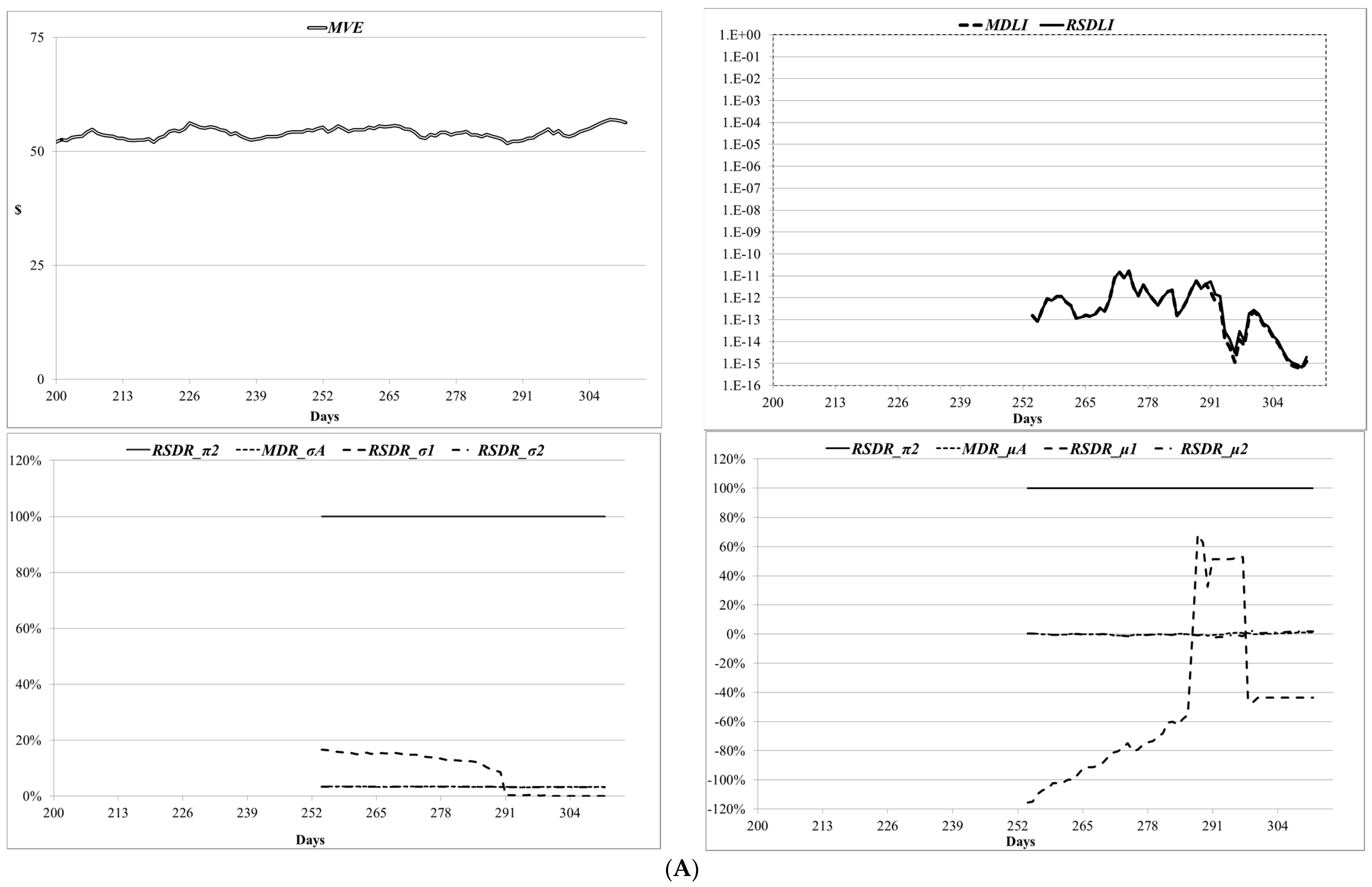
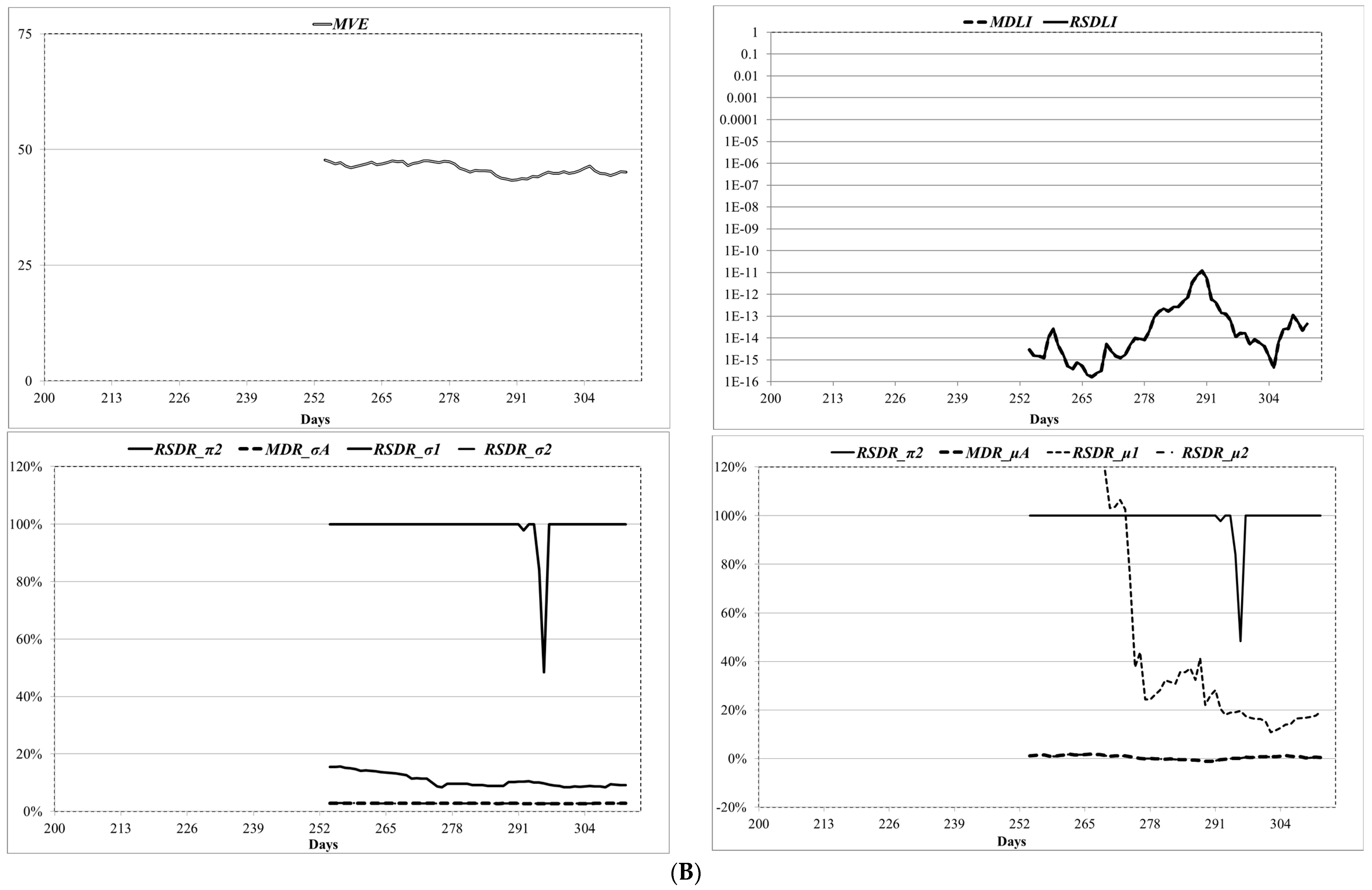
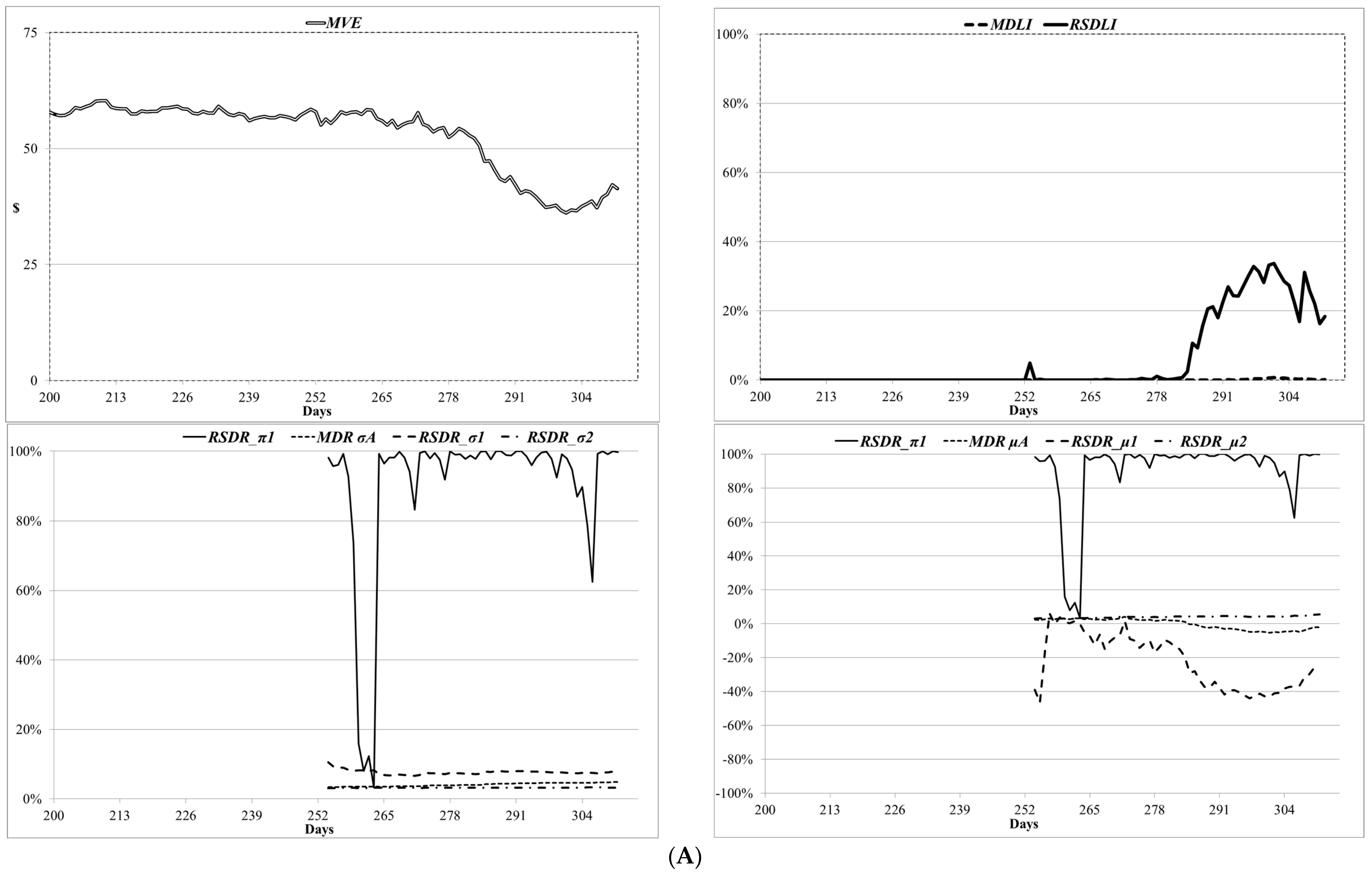
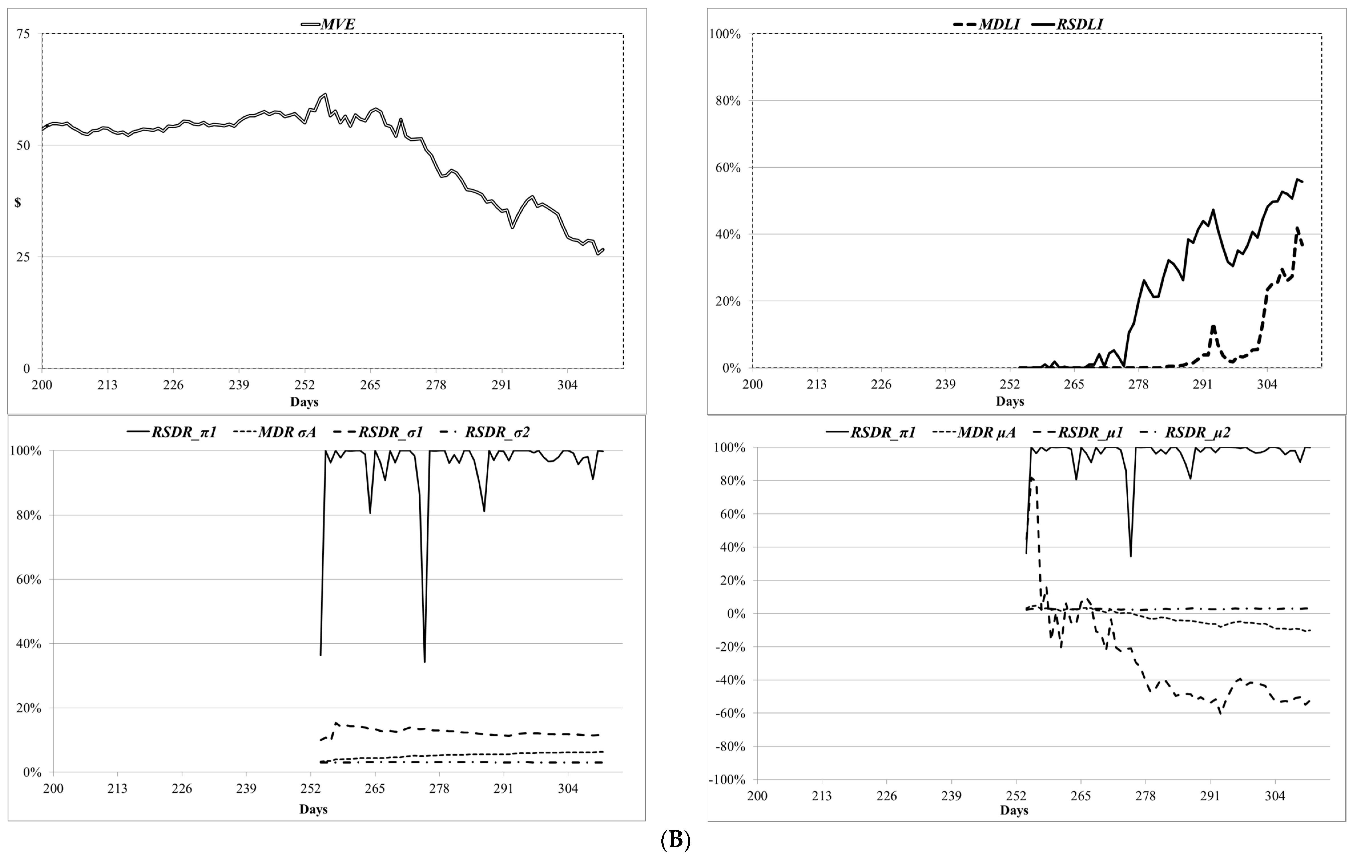
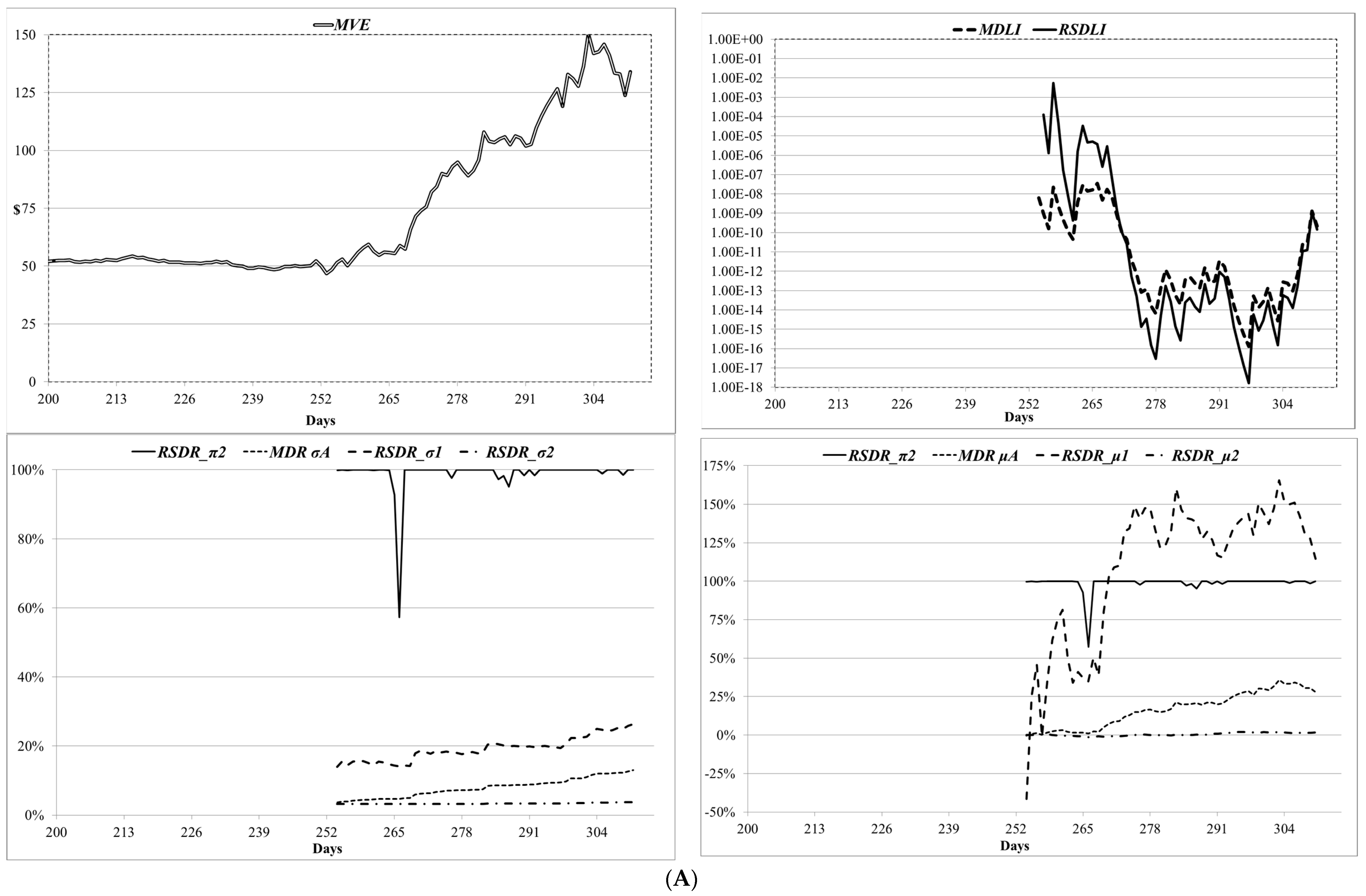
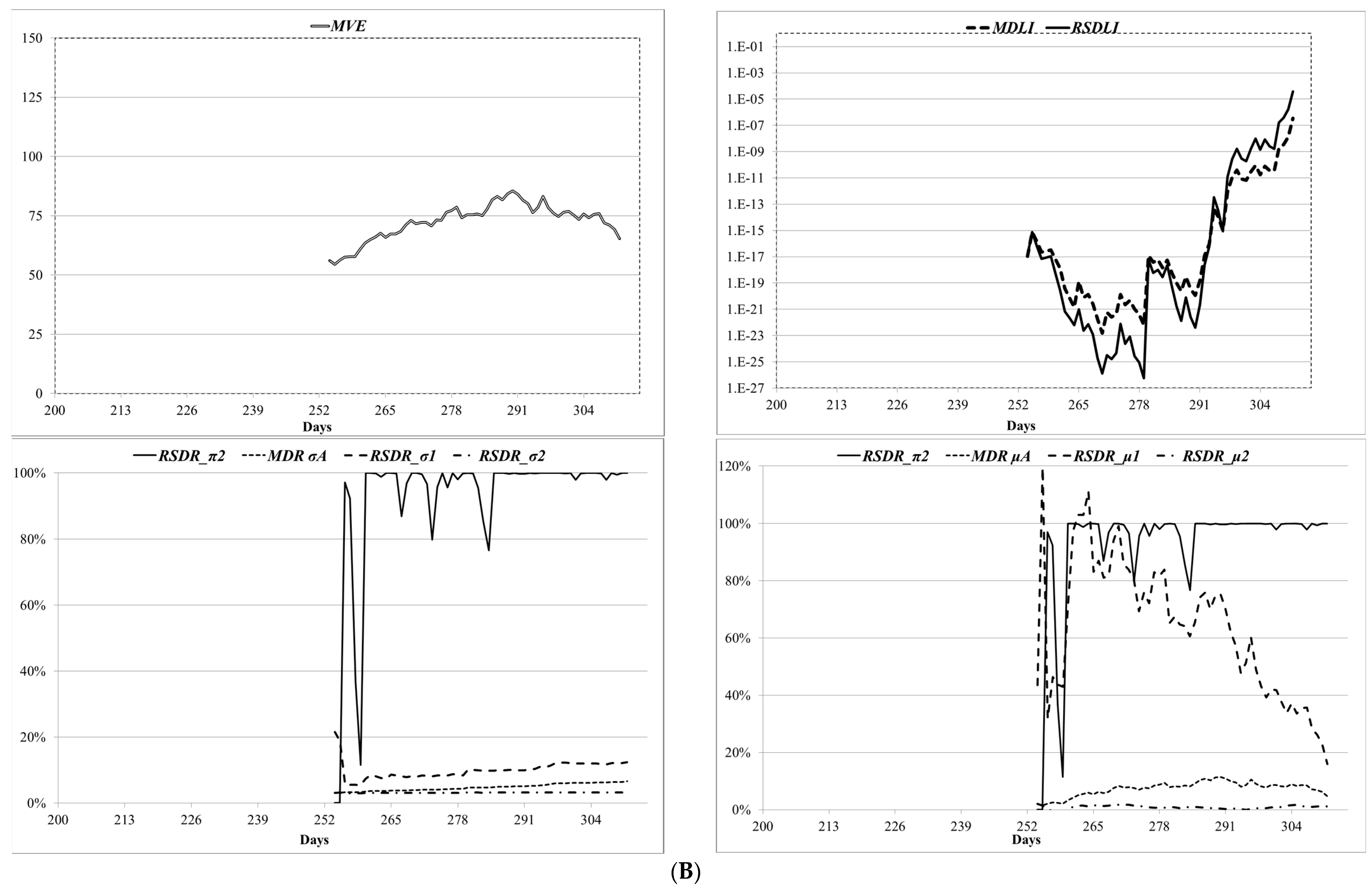
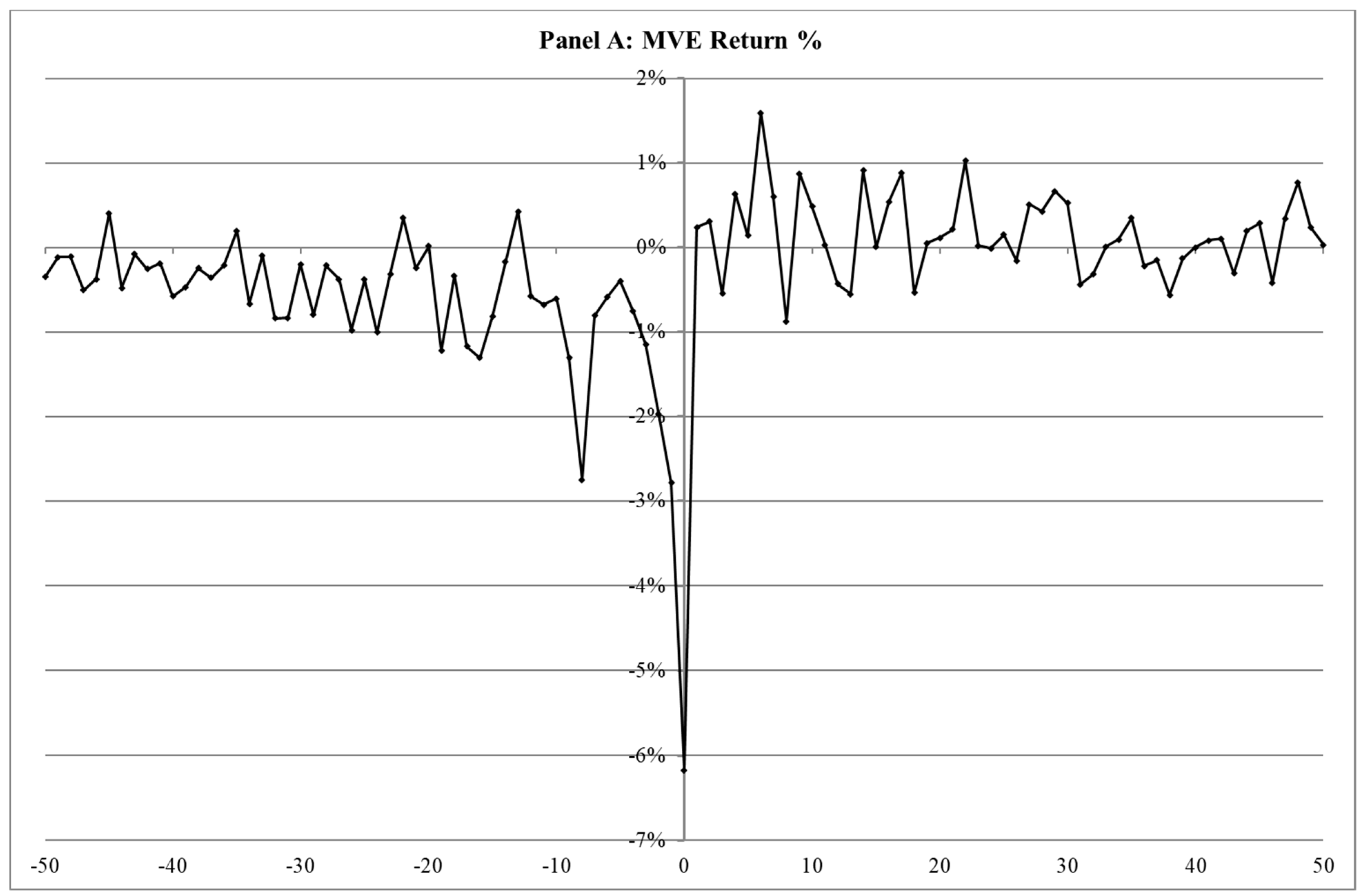
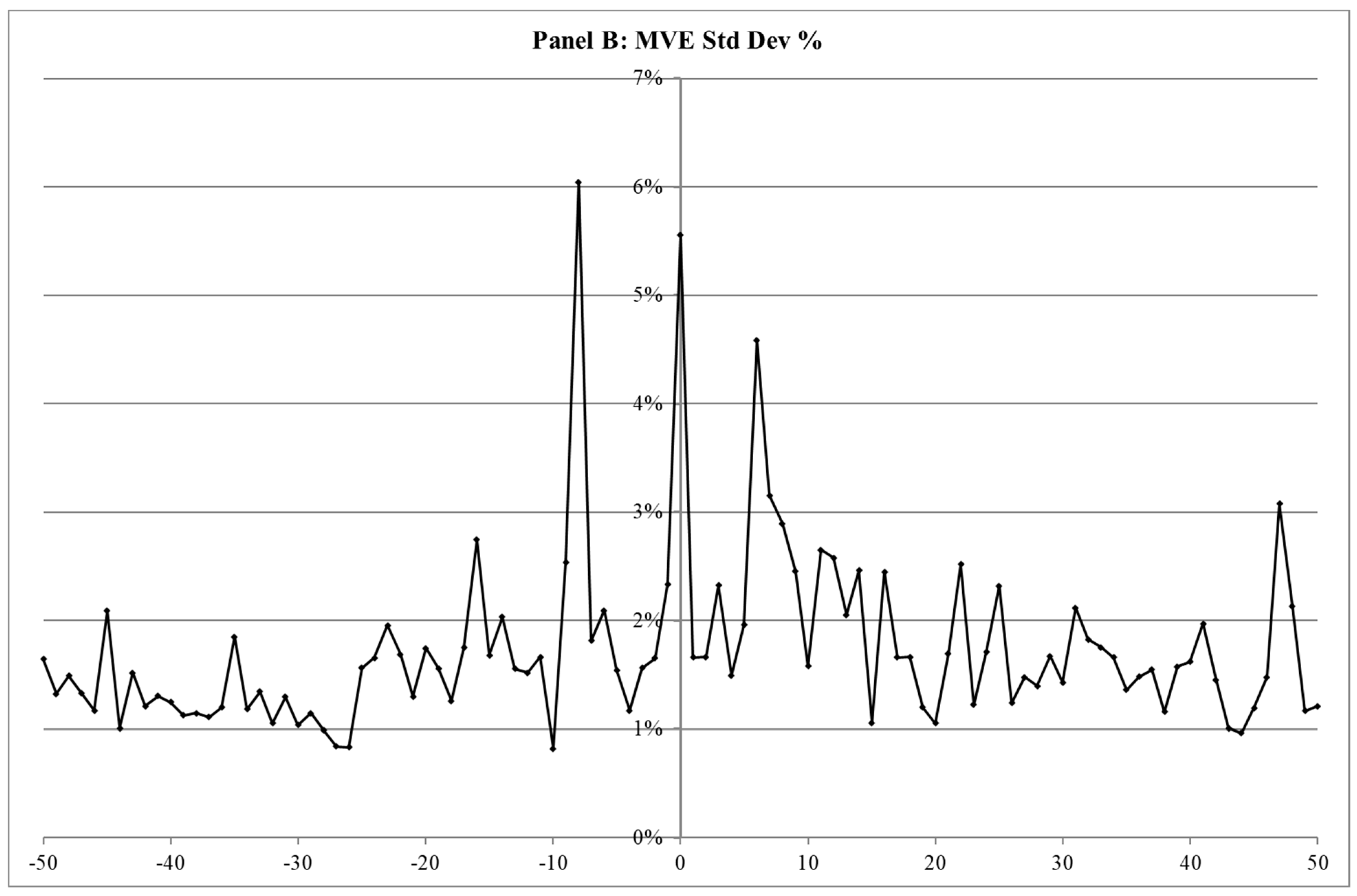
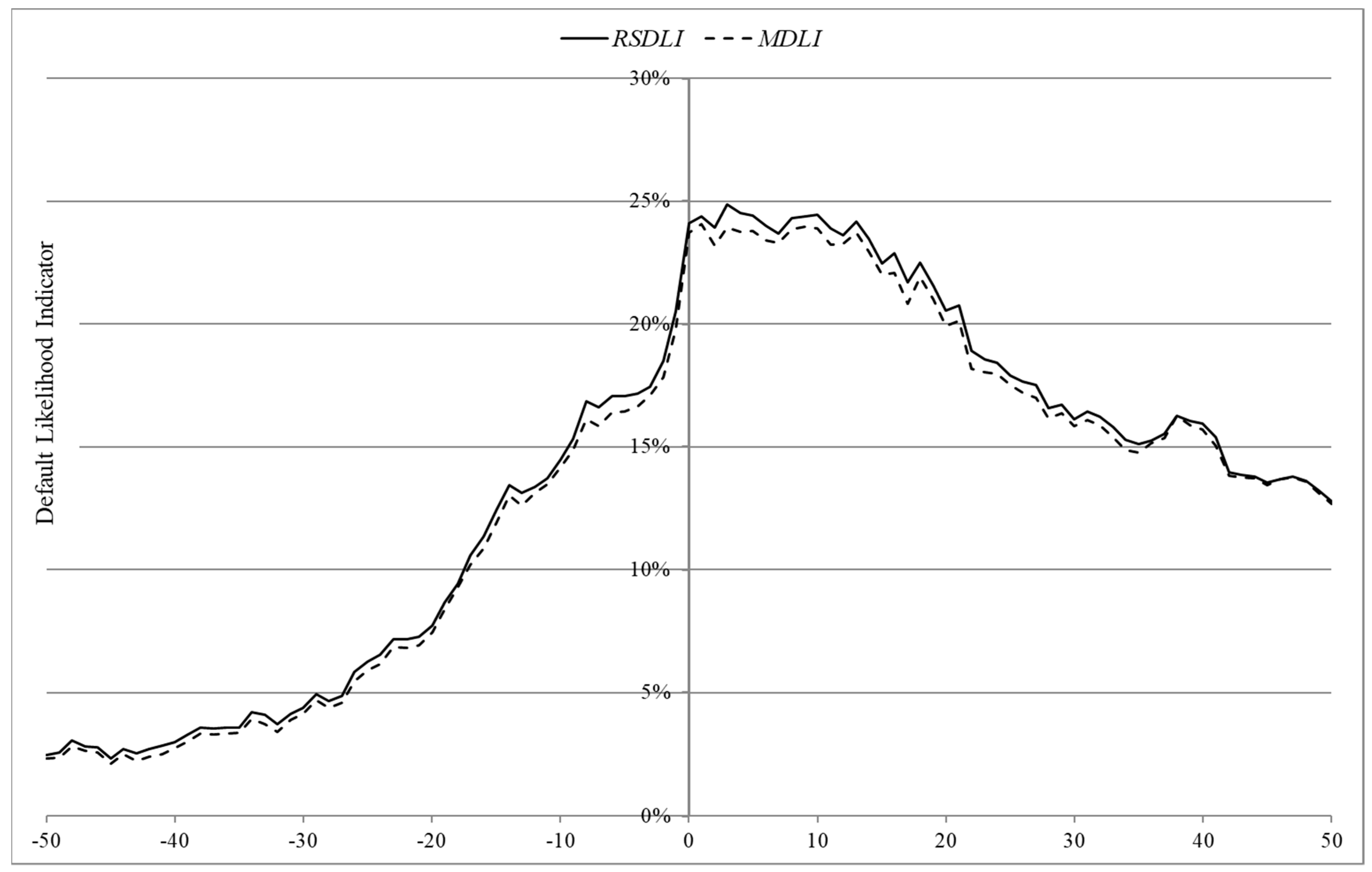
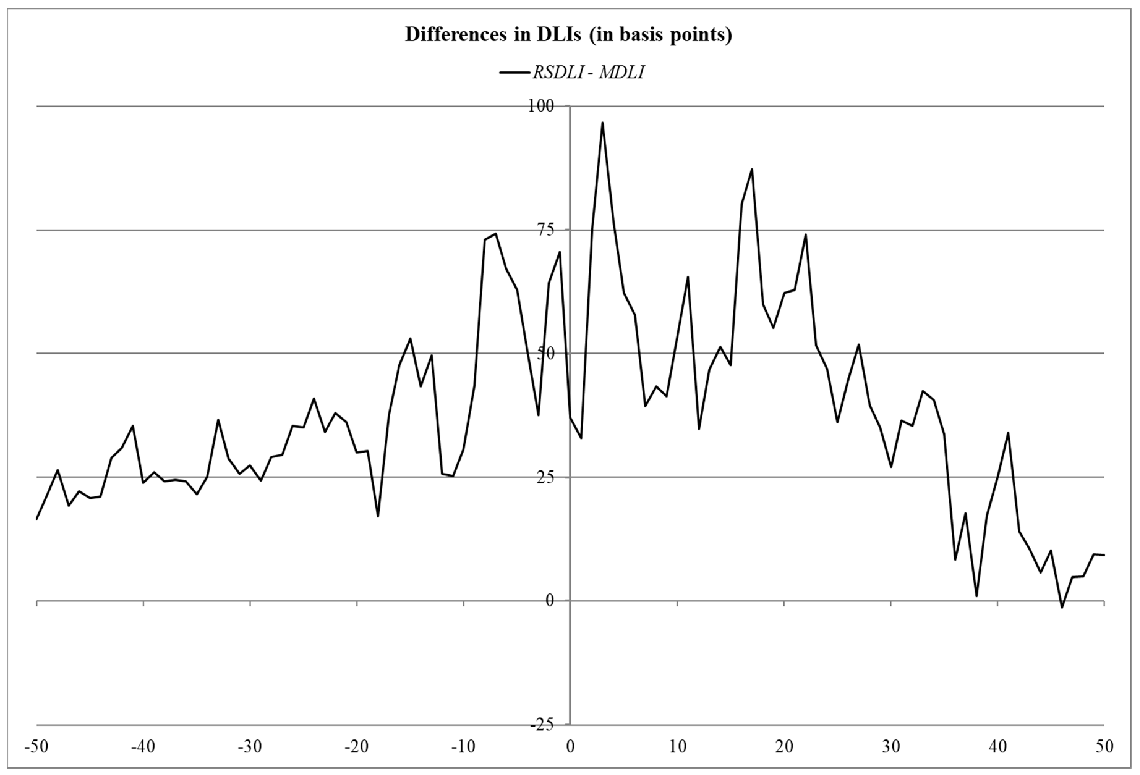
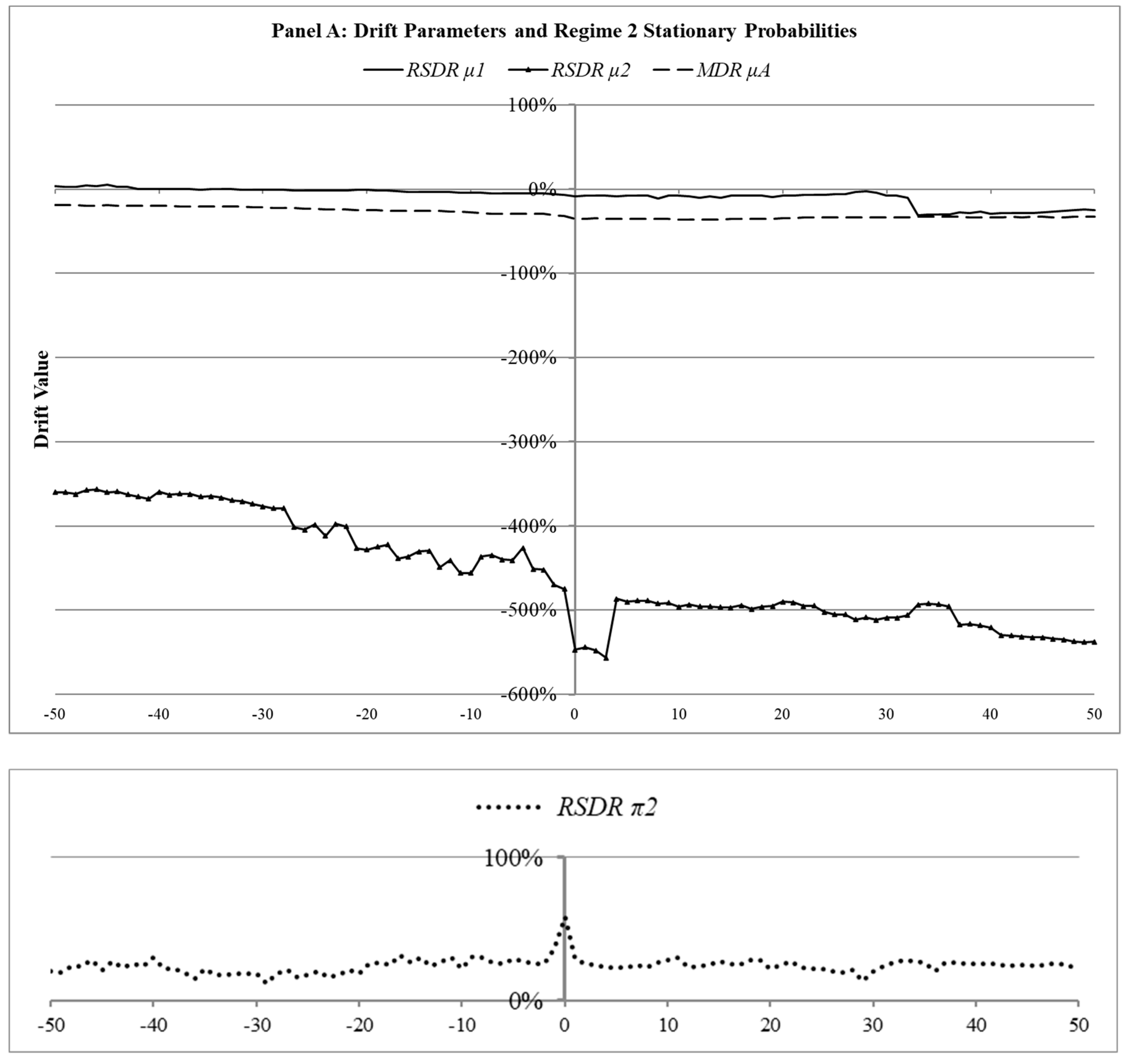
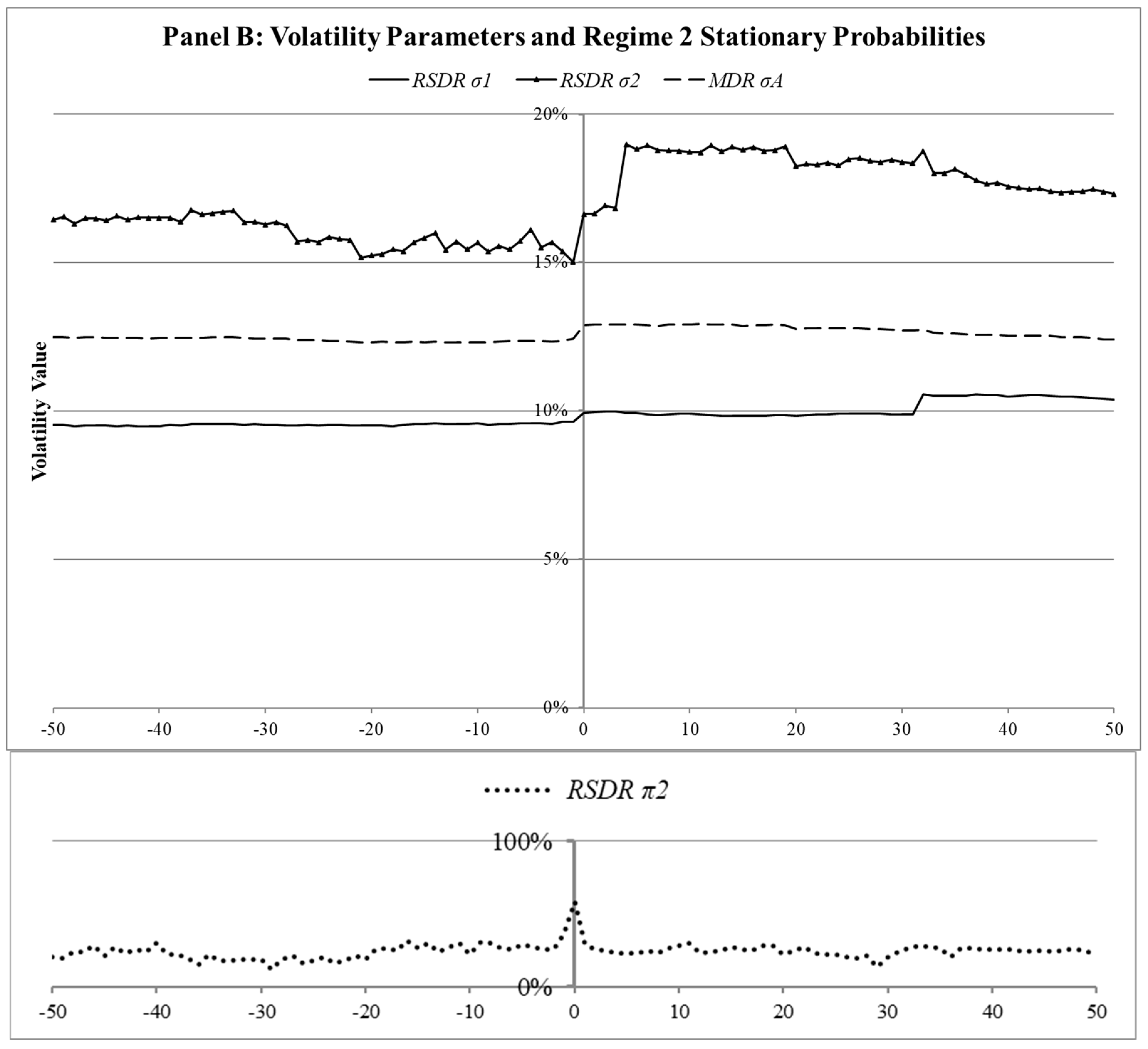
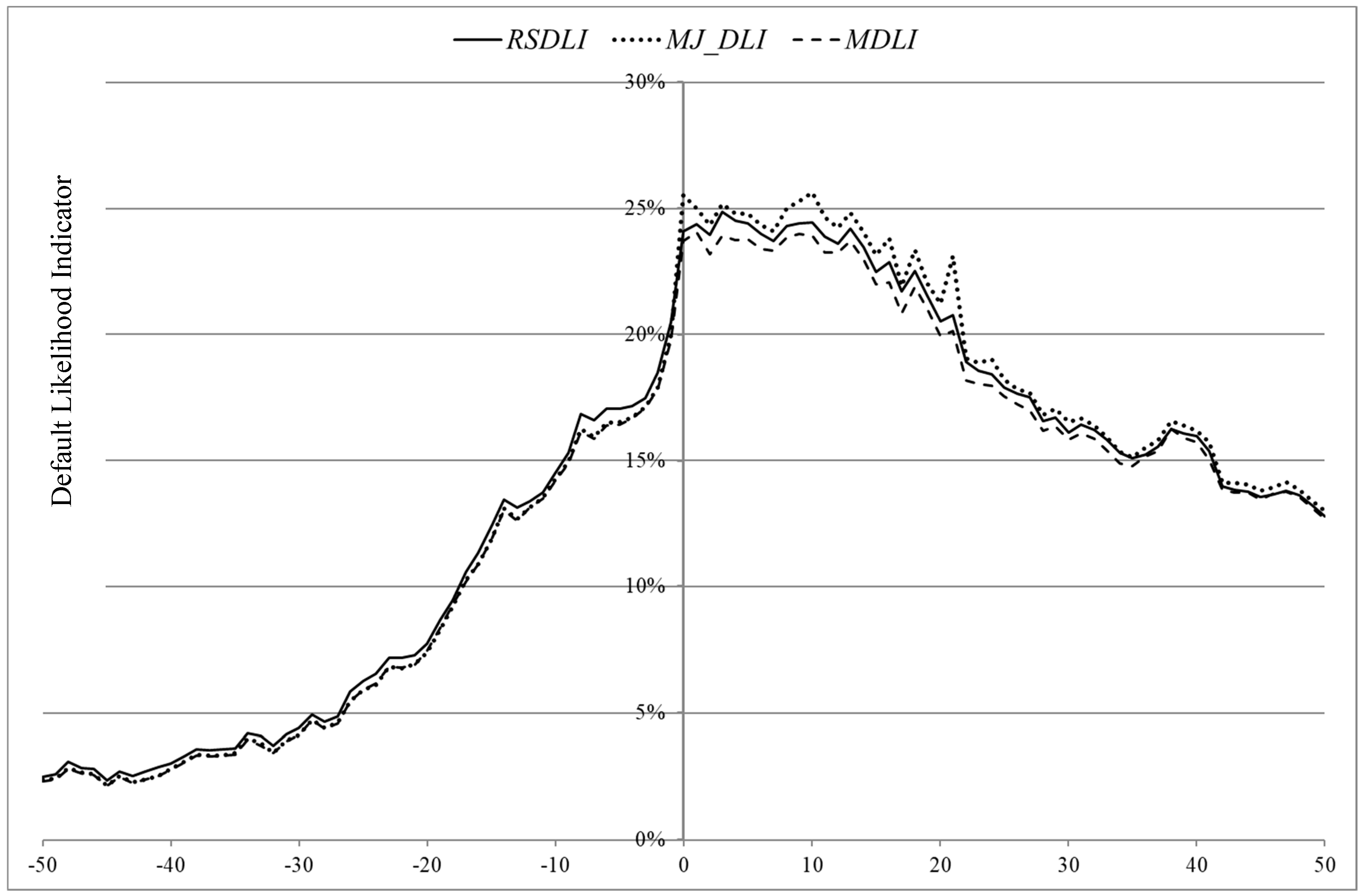
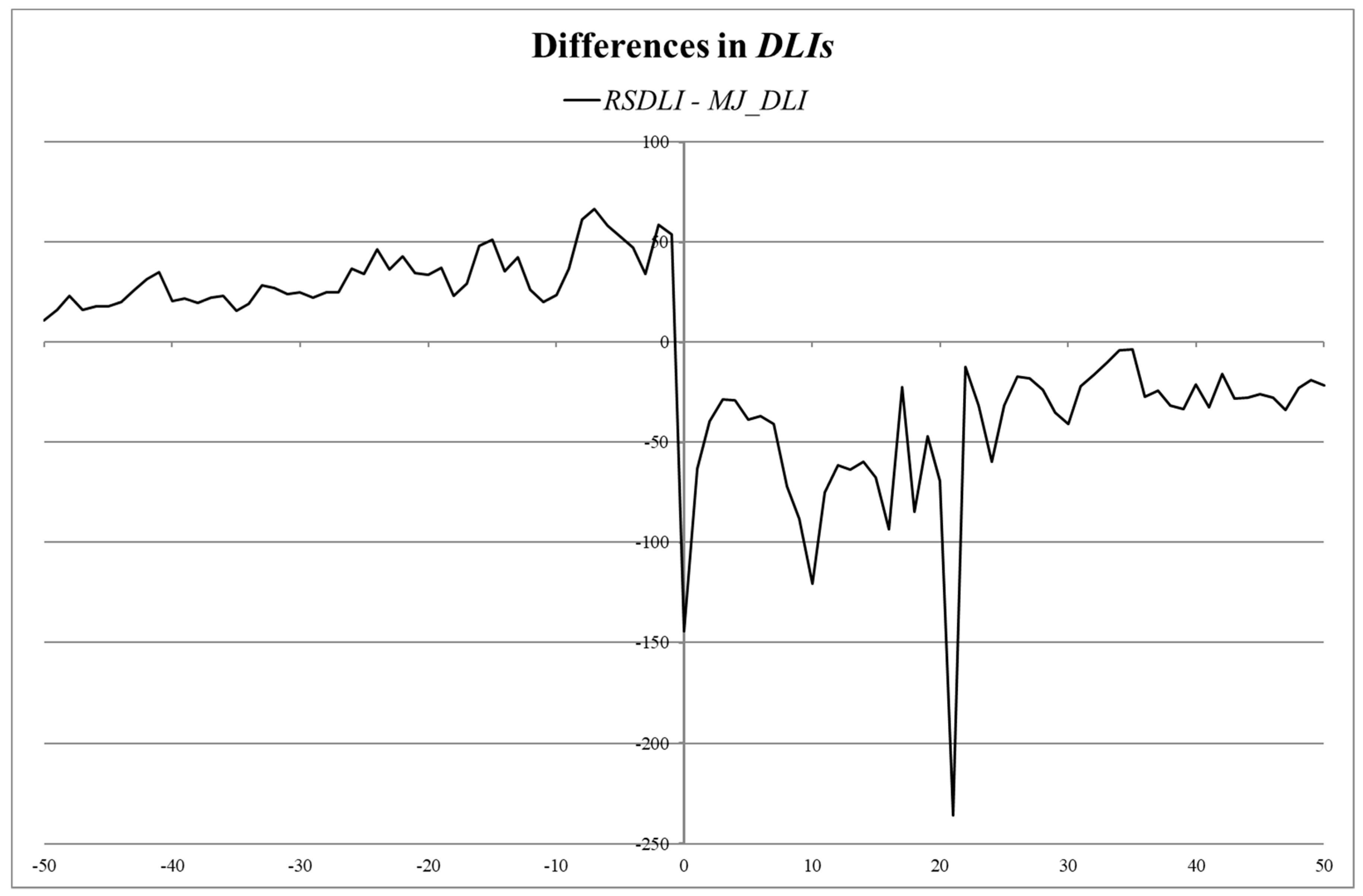
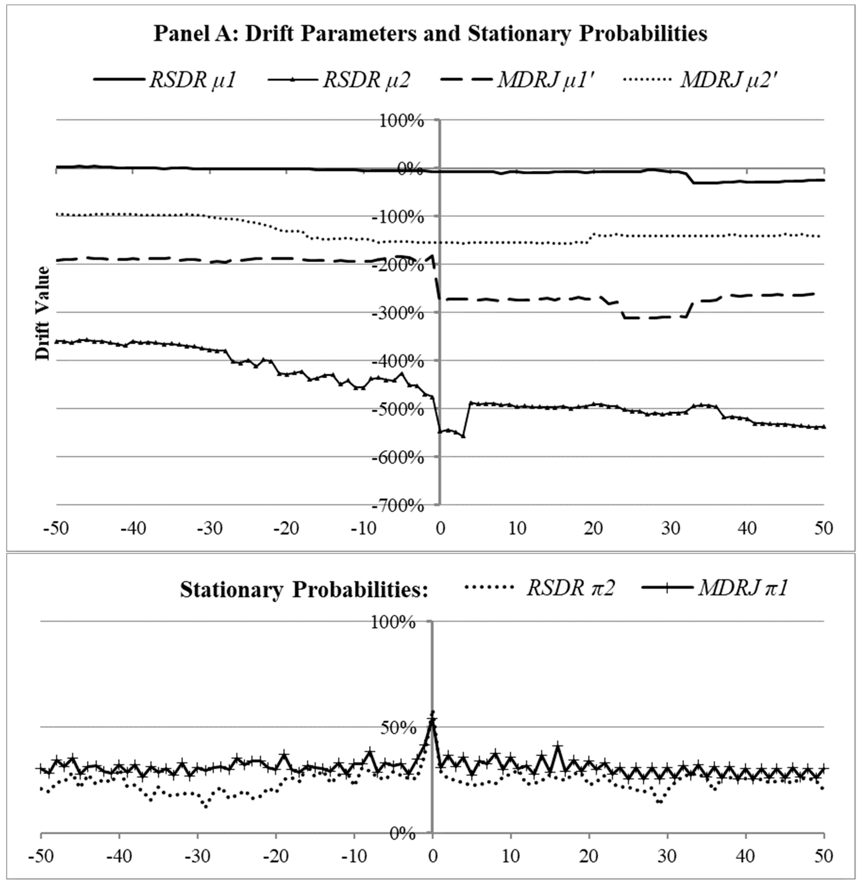
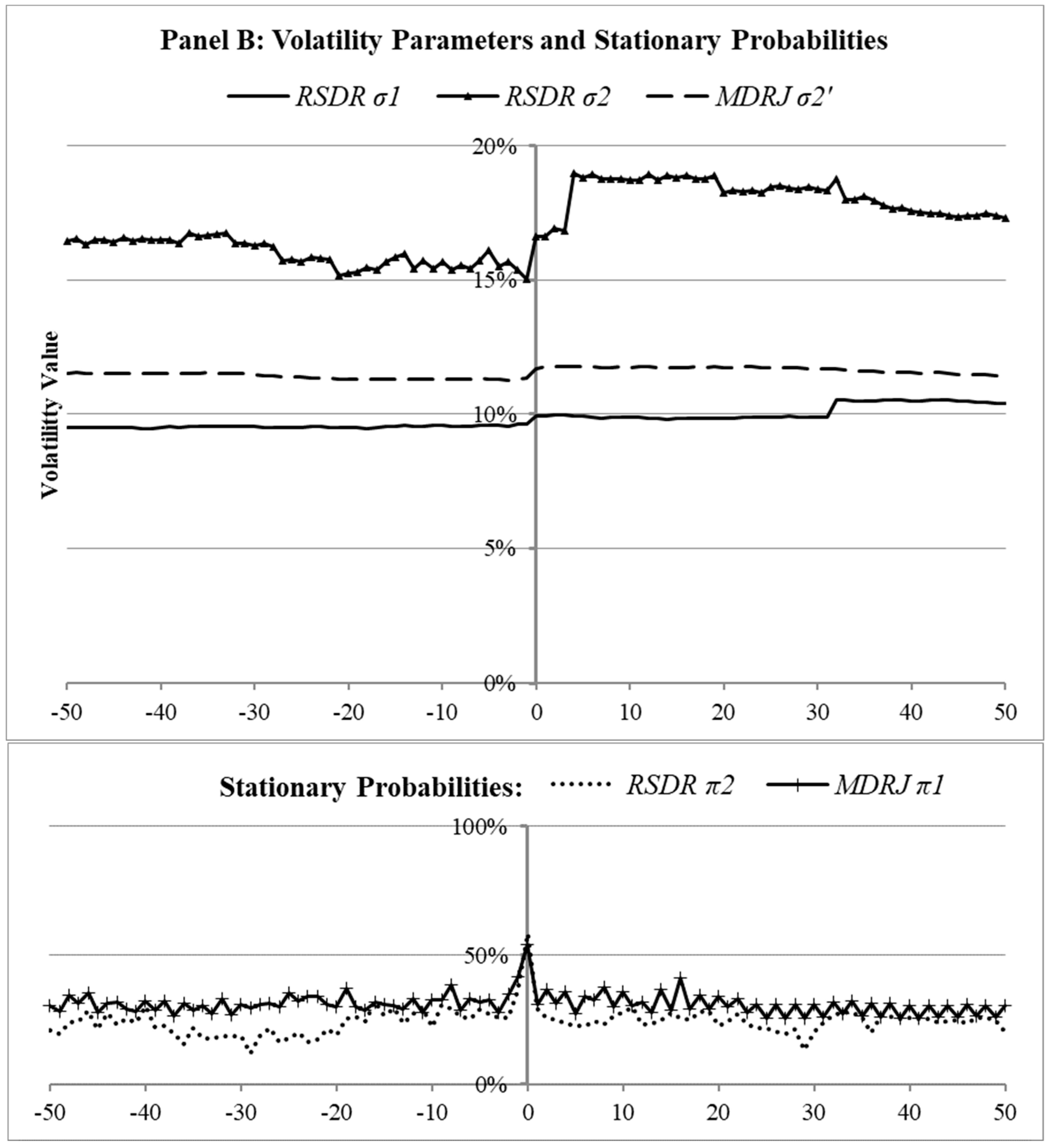
Table 1.
Changes in ratings by Egan Jones Ratings (1997–2002).
| EJR | Investment | Entire Database | Data Around Event | ||
|---|---|---|---|---|---|
| Rating | Grade? | Downgrade | Upgrade | Downgrade | Upgrade |
| AAA | yes | ||||
| AA+ | yes | 2 | 1 | ||
| AA | yes | 2 | 3 | 1 | |
| AA− | yes | 9 | 11 | 8 | 8 |
| A+ | yes | 28 | 26 | 23 | 23 |
| A | yes | 41 | 26 | 35 | 22 |
| A− | yes | 91 | 37 | 80 | 28 |
| BBB+ | yes | 92 | 63 | 78 | 46 |
| BBB | yes | 129 | 77 | 110 | 54 |
| BBB− | yes | 144 | 56 | 109 | 42 |
| BB+ | no | 115 | 52 | 94 | 38 |
| BB | no | 85 | 60 | 71 | 44 |
| BB− | no | 83 | 47 | 71 | 37 |
| B+ | no | 79 | 26 | 59 | 15 |
| B | no | 66 | 15 | 51 | 11 |
| B− | no | 54 | 3 | 37 | 3 |
| CCC+ | no | 4 | 3 | ||
| CCC | no | 36 | 3 | 21 | 3 |
| CCC− | no | ||||
| CC | no | 30 | 2 | 22 | 2 |
| C | no | 25 | 14 | ||
| D | no | 18 | 6 | ||
| Grand Total | 1133 | 507 | 893 | 377 | |
Egan Jones Ratings (EJR) uses 22 rating categories for corporate bond ratings (column “EJR Rating”). The lowest “Investment Grade” category is BBB−. Column “Entire Database” shows the distribution of upgrades and downgrades by rating category. Column “Data Around Event” shows the numbers of changes in ratings that can be matched with sufficient data in CRSP and Compustat to be used in the estimation of their default likelihood indicator. Specifically for CRSP, we require that firms have daily stock prices for the period of 504 before the event until 252 after the event. For Compustat, we require that the firm reports the financial variables for constructing the default boundary and market value of equity (used in later tables).
Table 2.
Descriptive statistics of input variables for the default risk models.
| Panel A: Market Value of Equity, Default Boundary and Risk-Free Rate by Rating Category | |||||||||||
| Category | Market Value of Equity (MVE) | Default Boundary | Risk-Free Rate | ||||||||
| (USD 1 million) | (USD 1 million) | ||||||||||
| Mean | Std. Dev. | Mean | Std. Dev. | Mean | Std. Dev. | ||||||
| AA− | 458,155 | 38,506 | 142,806 | 8410 | 2.00% | 0.10% | |||||
| A+ | 1,373,105 | 52,918 | 1,468,080 | 32,972 | 1.60% | 0.10% | |||||
| A | 1,428,275 | 110,874 | 795,030 | 13,402 | 1.90% | 0.10% | |||||
| A− | 1,610,407 | 107,046 | 692,493 | 15,849 | 2.00% | 0.10% | |||||
| BBB+ | 1,447,256 | 190,867 | 568,890 | 4531 | 1.80% | 0.10% | |||||
| BBB | 1,453,386 | 64,630 | 674,765 | 6014 | 1.70% | 0.10% | |||||
| BBB− | 1,281,199 | 188,001 | 429,357 | 5882 | 1.70% | 0.10% | |||||
| BB+ | 882,968 | 174,207 | 241,612 | 3411 | 1.60% | 0.20% | |||||
| BB | 555,183 | 181,663 | 114,661 | 1732 | 1.70% | 0.10% | |||||
| BB− | 366,656 | 116,614 | 100,282 | 506 | 1.50% | 0.20% | |||||
| B+ | 75,744 | 12,608 | 53,071 | 2315 | 1.70% | 0.10% | |||||
| B | 143,382 | 25,326 | 87,020 | 1808 | 2.00% | 0.10% | |||||
| B− | 57,374 | 15,759 | 70,393 | 1260 | 1.90% | 0.10% | |||||
| CCC | 25,151 | 7017 | 26,632 | 1159 | 2.00% | 0.10% | |||||
| CC | 36,224 | 3453 | 42,636 | 2924 | 2.30% | 0.10% | |||||
| C | 23,394 | 5299 | 34,462 | 5149 | 2.00% | 0.30% | |||||
| Panel B: Empirical Distribution of Market Value of Equity by Rating Category | |||||||||||
| Downgrade | Market Value of Equity (MVE) Return | ||||||||||
| Average | Std. Dev. | Skew. | Kurt. | pct 0% | pct 1% | pct 5% | pct 50% | pct 95% | pct 99% | pct 100% | |
| Category | Mean | Mean | Mean | Mean | Mean | Mean | Mean | Mean | Mean | Mean | Mean |
| AA− | 0.00% | 1.40% | 4.02 | 41.98 | −4.60% | −2.40% | −1.70% | −0.10% | 1.80% | 2.80% | 13.90% |
| A+ | 0.00% | 0.70% | 0.11 | 2.57 | −2.40% | −1.70% | −1.10% | 0.00% | 1.00% | 1.80% | 2.70% |
| A | 0.00% | 0.90% | 0.29 | 1.19 | −2.40% | −2.00% | −1.40% | 0.00% | 1.40% | 2.10% | 4.10% |
| A− | −0.10% | 0.80% | −0.27 | 0.90 | −3.10% | −2.40% | −1.30% | 0.00% | 1.30% | 1.80% | 2.60% |
| BBB+ | −0.20% | 1.00% | −0.96 | 5.09 | −6.00% | −2.90% | −1.60% | −0.10% | 1.40% | 2.10% | 2.40% |
| BBB | −0.10% | 0.70% | −0.48 | 4.64 | −3.90% | −1.70% | −1.10% | −0.10% | 1.10% | 1.60% | 2.30% |
| BBB− | −0.20% | 0.90% | −0.66 | 2.07 | −4.20% | −3.00% | −1.50% | −0.20% | 1.10% | 1.70% | 2.20% |
| BB+ | −0.30% | 1.10% | −0.80 | 4.41 | −5.90% | −3.40% | −1.80% | −0.20% | 1.40% | 1.90% | 2.80% |
| BB | −0.40% | 1.60% | −0.86 | 3.44 | −8.60% | −5.30% | −2.90% | −0.30% | 2.10% | 2.90% | 3.90% |
| BB− | −0.40% | 1.80% | −1.25 | 5.99 | −10.30% | −6.50% | −2.90% | −0.30% | 2.00% | 3.60% | 4.30% |
| B+ | −0.20% | 1.00% | −0.73 | 2.82 | −4.90% | −3.60% | −1.80% | −0.20% | 1.30% | 2.00% | 2.70% |
| B | −0.30% | 1.40% | −0.24 | 0.29 | −4.70% | −3.70% | −2.70% | −0.20% | 1.80% | 2.50% | 4.00% |
| B− | −0.40% | 1.40% | −0.59 | 8.16 | −8.70% | −4.00% | −2.30% | −0.30% | 1.70% | 3.00% | 6.00% |
| CCC | −0.40% | 1.80% | −1.36 | 11.05 | −12.20% | −4.40% | −3.20% | −0.40% | 2.40% | 3.40% | 4.90% |
| CC | −0.10% | 1.60% | −0.70 | 4.50 | −8.50% | −5.00% | −2.50% | 0.00% | 2.10% | 3.70% | 5.70% |
| C | −0.30% | 2.10% | −0.52 | 6.41 | −11.70% | −5.50% | −3.30% | −0.40% | 2.90% | 4.90% | 7.70% |
Panel A shows the descriptive statistics for each rating category with more than ten observations with usable input data (market value of equity (MVE) and default boundary). MVE for each rating category is the sum of individual firms’ MVEs (product of daily closing price and number of shares outstanding) that are downgraded to that category. Default boundary is the sum of short-term debt plus one-half of long-term debt (data49 + 0.5 × data51) from CCM: CRSP Compustat merged database. The risk-free rate is obtained from Kenneth French’s website (http://mba.tuck.dartmouth.edu/pages/faculty/ken.french/ (accessed on 15 December 2023)). In Panel B, the average, standard deviation (std. dev.), skewness (skew) and kurtosis (kurt) of the MVE return are given. The numbers given (“Mean”) represent the time-series average over all observations (from until ) of each variable across rating categories. “Pct x %” stands for the x-th percentile of the distribution of the market value of equity returns.
Disclaimer/Publisher’s Note: The statements, opinions and data contained in all publications are solely those of the individual author(s) and contributor(s) and not of MDPI and/or the editor(s). MDPI and/or the editor(s) disclaim responsibility for any injury to people or property resulting from any ideas, methods, instructions or products referred to in the content. |
© 2024 by the authors. Licensee MDPI, Basel, Switzerland. This article is an open access article distributed under the terms and conditions of the Creative Commons Attribution (CC BY) license (https://creativecommons.org/licenses/by/4.0/).
Share and Cite
MDPI and ACS Style
Milidonis, A.; Chisholm, K. The Regime-Switching Structural Default Risk Model. Risks 2024, 12, 48. https://doi.org/10.3390/risks12030048
AMA Style
Milidonis A, Chisholm K. The Regime-Switching Structural Default Risk Model. Risks. 2024; 12(3):48. https://doi.org/10.3390/risks12030048
Chicago/Turabian StyleMilidonis, Andreas, and Kevin Chisholm. 2024. "The Regime-Switching Structural Default Risk Model" Risks 12, no. 3: 48. https://doi.org/10.3390/risks12030048
Note that from the first issue of 2016, this journal uses article numbers instead of page numbers. See further details here.