1. Introduction
Insurance is the activity by which an individual or enterprise exchanges an uncertain (financial) loss with a certain (financial) loss. The former is the outcome of an event for which the insured individual or enterprise has received coverage via an insurance policy; the latter is the premium that the insured has to pay to receive this coverage. When such an event occurs, the insured may formally request coverage (monetary or in-kind) in line with the policy terms and conditions, which constitutes the insurance claim.
It is therefore clear that claims are key components of the insurance activity as they essentially comprise the realization of the insurance product/service. Due to the uncertainty of (future) claims occurrence, it is in the interest of the insurers to carefully frame their claims expectations and provisions. Consequently, they pursue claims forecasting. The accurate forecasting of insurance claims is important for several reasons.
First, claims constitute the basis of pricing. In insurance, contrary to other services, the validity of the pricing is confirmed, and the adequacy of the premium is proved only after the experience has been recorded. Traditional pricing is based on historical data; however, it is the occurrence of incidents in the future that determines whether the estimated burning cost was correct or not. Hence, if the claims experience has not been properly embedded in the pricing models, the (pure) premium may not be sufficient to cover the total claims (incurred or paid) and this could lead to a loss-making activity—if the premium charged is too low. In contrast, it could result in the loss of customers—in the case where the premium charged is too high.
Second, future claims occurrence is important for the compilation of the business plan as claims affect the future profitability of the company. In fact, the claims experience is probably the most significant determinant of the operational profitability of the insurance company. This is due to the fact that when compiling the business plan, an insurance company projects the future premia and the future claims over a period of years. Future premia are based primarily on sales forecasts, the evolution of inflation (ideally the one related to the insurance coverage under examination), as well as the projected claims experience. Expected future claims are based on the historical claims experience as well as on assumptions on the development of claims; this may be decomposed to the development of claims frequency and severity.
Finally, having a forward look in claims is a prerequisite of their risk and solvency assessment process and report, which depicts the risk appetite of the insurer and thus the capital required for the solvency of the insurer. As a matter of fact, it usually requires (one of) the biggest portions of capital (allocations). Indeed, insurers assume the risks that individuals and enterprises want to transfer, hedge, or mitigate. A claim is filed when a covered event (the assumed risk) has occurred. A higher risk appetite indicates the assumption of higher risk and thus higher claim anticipation. This leads to higher (economical) capital required for the absorption of this risk.
The conventional forecasting approaches attempt to either repeat the historical (growth) pattern of claims in the future–with potential seasonality and respective premia considered–or match the claims frequency and severity experience of the insurance company with a known probability distribution function. Smaller claims exhibit higher frequency, whereas large claims have a (much) smaller frequency. To improve the precision of the forecasting, large claims are pooled separately from the small claims and different probability distribution functions are used to best fit the claims frequency and severity of the two pools of claims.
Machine Learning approaches offer an alternative route to claims forecasting. The contribution of ML (artificial intelligence—AI) in insurance globally and in claims prediction specifically has been recognized by practitioners—who have spotted a wide range of ML applications in insurance—spreading over almost all its processes, such as claims processing, claims fraud detection, claims adjudication, claim volume forecasting, automated underwriting, submission intake, pricing and risk management, policy servicing, insurance distribution, product recommendation/personalized offers, assessor assistance, property (damage) analysis, automated inspections, customer lifetime value prediction/customer retention/lapse management, speech analytics, customer segmentation, workstream balancing for agents, and self-servicing for policy management (
Seely 2018;
Somani 2021). A report from the Organization for Economic Cooperation and Development (
OECD 2020) subscribes to this point of view as it identifies the increasing number of ML (AI) applications in insurance, which are enabled through the widespread collection of big data and their analysis. The report pinpoints marketing, distribution and sales, claims (verification and fraud), pricing, and risk classification as broader areas of ML utilization. It further addresses some attention points, such as policy and regulation with regards to the use of ML in insurance, with emphasis among others in privacy and data protection, market structure, risk classification, and explainability of ML. The implementation of ML (AI) methods in these sectors of the insurance operations, along with the relevant worries on ethical and societal challenges have been recorded by
Grize et al. (
2020),
Banks (
2020),
Ekin (
2020), and
Paruchuri (
2020). The reports of
Deloitte (
2017),
SCOR (
2018),
Keller et al. (
2018), and
Balasubramanian et al. (
2021) identify similar applications of ML as they pave the future of insurance.
In this paper, we employ a series of Machine Learning algorithms (Support Vector Machines–SVM, Decision Trees, Random Forests, and Boosting) to forecast the average (mean) insurance claims amount per insured car per quarter and identify a subset of variables that are the most relevant in determining the average claims amount. The claims data come from the motor portfolio of an insurance company (operating in Athens, Greece) for the period between 2008–2020.
This approach is novel as it investigates the impact of two new-to-the-literature sets of variables, namely variables relevant to weather conditions and car sales, on the evolution of motor insurance claims with the use of ML techniques to forecast motor insurance claims. More specifically, insurers attempt to forecast motor insurance claims based on their own experience, which depends on the particulars of the vehicle and the driver. However, there is a third component recorded as “road” (
Norman 1962;
Dimitriou and Poufinas 2016). “Road” describes (environmental) factors such as time of the day, day of the week, weather conditions, type of road design and surface, lighting and visibility, etc. It is essentially a set of factors that refer to all factors that can affect the incidence of road traffic accidents other than the factors that are relevant to the driver (road user) and the vehicle. “Road” encompasses all factors that are not captured by the driver and the vehicle. Driver, vehicle, and “road” are essentially sets of factors. Consequently, “road” captures (among others) the condition of the terrain, which is impacted by the weather conditions (among other parameters). Furthermore, “road” captures the road usage, which is affected by the number of vehicles using it. This is, in turn, impacted by the new and used car sales. As a result, we feel we unveil the attributes of one important motor accident component, namely, “road”, which is novel in motor insurance claim forecasting.
We trust this is useful in the hands of insurers as they now have an additional set of factors to perform motor claim forecasting. When performing motor claim forecasting, some insurers, among which the insurer that provided the dataset for this study, rely on the address that the insured vehicle is registered; hence, they do not consider the area where the accident took place. As a result, the “road” component is not captured. Our approach offers a way to forecast motor insurance claims with the inclusion of two sets of parameters that impact this component: weather conditions and car sales.
2. Literature Review
The bulk of the literature on the applications of machine learning in insurance is relatively recent (post 2019) and although they cover a wide range of topics relevant to the insurance activity, there is ample room for further research. The main literature strands focus on claims, reserving, pricing, capital requirements–solvency, coverage ratio, acquisition, and retention. We group them into two main categories; actuarial and risk management that incorporates the first four (claims, reserving, pricing, and capital requirements–solvency) and customer management, which incorporates the last three (coverage ratio, acquisition, and retention). As the second category is not relevant to our study, we do not present it in detail. The interested reader may look at
Mueller et al. (
2018) for the coverage ratio;
Boodhun and Jayabalan (
2018) and
Qazi et al. (
2020) for acquisition; and
Grize et al. (
2020) and
Guillen et al. (
2021) for retention.
The literature that is relevant to actuarial and risk management issues addresses the main functions of the insurance activity and is thus related to actuarial science and risk management. In fact, insurance is the assumption and management of risks that individuals or enterprises wish to transfer or mitigate. These functions entail the monitoring of the claims/risks evolution, the determination of the required reserves, the estimation of the appropriate tariff rates as well as the calculation of the capital that is required to ensure the solvency of the insurer. The analysis of these literature strands follows.
2.1. Claims/Risks
Fauzan and Murfi (
2018) focus on the forecasting of motor insurance accident claims via ML methods with an emphasis on missing data.
Rustam and Ariantari (
2018) use ML approaches to predict the occurrence of motor insurance claims based on their claim history (with data stemming from an Indonesian motor insurer).
Pesantez-Narvaez et al. (
2019) attempt to predict the existence of accident claims with the use of ML techniques on telematics data (coming from an insurance company) with an emphasis on driving patterns (total annual distance driven and percentage of distance driven in urban areas).
Qazvini (
2019) employs ML methods to predict the number of zero claims (i.e., claims that have not been reported) based on telematics data (on French motor third party liability).
Bermúdez et al. (
2020) apply ML approaches to model insurance claim counts with an emphasis on the overdispersion and the excess number of zero claims, which may be the outcome of unobserved heterogeneity.
Bärtl and Krummaker (
2020) attempt to predict the occurrence and the magnitude of export credit insurance claims with the use of ML techniques. The models employed produce satisfactory results for the former but not so satisfactory for the actual claim ratios—with accuracy, Cohen’s κ and R
2 were used to assess model performance.
Knighton et al. (
2020) focused on forecasting flood insurance claims with ML models that applied hydrologic and social demographic data to realize that the incorporation of such data can improve flood claim prediction.
Hanafy and Ming (
2021) apply ML approaches to predict the occurrence of motor insurance claims (over the portfolio of Porto Seguro, a large Brazilian motor insurer).
Selvakumar et al. (
2021) concentrated on the prediction of the third-party liability (motor insurance) claim amount for different types of vehicles with ML models (on a dataset derived from Indian public insurance companies).
Some recent articles utilize the data collected through telematics. More specifically,
Duval et al. (
2022) used ML models to come up with a method that indicates the amount of information—collected via telematics with regards to the policyholders’ driving behavior—that needs to be (optimally) retained by insurers to (successfully) perform motor insurance claim classification.
Reig Torra et al. (
2023) also capitalized on the data provided by telematics and used the Poisson model, along with some weather data, to forecast the expected motor insurance claim frequency over time. They found that weather conditions do affect the risk of an accident.
Masello et al. (
2023) used the information collected via telematics and employed ML methods to assess the predictive ability of driving contexts (such as road type, weather, and traffic) to driving risks/safety (such as near-misses, speeding, and distraction events), which, in turn, affected the exposure to/occurrence of accidents and thus motor insurance claims.
Pesantez-Narvaez et al. (
2021) compared the ability of ML models to detect rare events (on a third-party liability motor insurance dataset) to realize that RiskLogitboost regression exhibits a superior performance over other methods.
Shi and Shi (
2022) employed ML approaches on property insurance claims to develop rating classes and estimate rating relativities for a single insurance risk; perform predictive modeling for multivariate insurance risks and unveil the impact of tail-risk dependence; and price new products.
In a different direction—that of fraud detection—
Pérez et al. (
2005) applied ML approaches (on a motor insurance portfolio) in a different context, which still pertained to claims; they focused on the detection of fraudulent claims in motor insurance by properly classifying suspicious claims.
Kose et al. (
2015) employed ML approaches for the detection of fraudulent claims or abusive behavior in healthcare insurance via an interactive framework that incorporates all the interested parties and materials involved in the healthcare insurance (claim) process. On the same topic,
Roy and George (
2017) used ML methods to detect fraudulent claims in motor insurance.
Wang and Xu (
2018) employed ML models that incorporate the (accident) information embedded in the text of the claims to detect potential claim fraud in motor insurance.
Dhieb et al. (
2019,
2020) applied ML techniques to automatically identify motor insurance fraudulent claims and sort them into different fraud categories with minimal human intervention, along with alerts for suspicious claims.
A series of papers implemented ML approaches in health management/insurance.
Bauder et al. (
2016) introduced ML approaches to tackle a different topic of insurance claims, thereby allowing them to spot the physicians that post a potentially anomalous behavior (pointing out misuse, fraud, or ignorance of the billing procedures) in health (medical) insurance claims (with data taken from the USA Medicare system) and for which additional investigation may be necessary.
Hehner et al. (
2017) highlighted the merits of the introduction of ML (AI) in hospital claims management, which can be summarized as savings for both the insurers and the insured as ML algorithms result in increased efficiency and well-informed decision-making to the benefit of all interested parties.
Rawat et al. (
2021) applied ML methods to analyze claims and conclude on a set of factors that facilitate claim filing and acceptance.
Cummings and Hartman (
2022) propose a series of ML models that provide insurers the ability to forecast Long Term Care Insurance (LTCI) claim rates and thus better their capacity to operate as LTCI providers.
2.2. Reserving
Baudry and Robert (
2019) developed a ML method to estimate claims reserves with the use of all policy and policyholder covariates, along with the information pertaining to a claim from the moment it has been reported and compared their results with those generated via chain ladder.
Elpidorou et al. (
2019) employed ML techniques to introduce a novel Bornhuetter–Ferguson method as a variant of the traditional chain ladder method used for reserving in non-life (general) insurance through which the actuary can adjust the relative ultimate reserves with the use of externally estimated relative ultimate reserves. In the same direction,
Bischofberger (
2020) utilized ML methods to extend the chain ladder method via the estimated hazard rate for the estimation of non-life claims reserves.
The outperformance (in 4 out of 5 lines of business studied) of ML algorithms over traditional actuarial approaches in estimating loss reserves (future customer claims) is evidenced by the work of
Ding et al. (
2020). Similarly,
Gabrielli et al. (
2020) explore the merit of the introduction of ML approaches to traditional actuarial techniques in improving the non-life insurance claims reserving (prediction).
2.3. Pricing
Gan (
2013), in a comparatively early work, priced the guarantees (i.e., finds the market value and the Greeks) of a large portfolio of variable annuity policies (generated by the author) via ML techniques.
Assa et al. (
2019) used ML approaches to study the correct pricing of deposit insurance by improving the implied volatility calibration to avoid mispricing due to arbitrage.
Grize et al. (
2020) unveiled the role of ML algorithms in (online) motor liability insurance pricing and, at the same time, increased the issue of interpretability.
Henckaerts et al. (
2021) capitalized on ML methods to price non-life insurance products based on the frequency and severity of claims; their results are superior to the ones produced by the traditionally employed generalized linear models (GLMs).
Kuo and Lupton (
2020) explained that the wider adoption of ML techniques (over GLMs) in property and casualty insurance pricing depends very much on their reduced (perceived) transparency. They recommend increased interpretability to overcome this hurdle. These concerns are also addressed in
Grize et al. (
2020).
Blier-Wong et al. (
2020) performed a literature review on the application of ML methods on the property and casualty insurance actuarial tasks and in pricing and reserving. They drafted potential future applications and research in the field and noticed that there can be three main challenges: interpretability, prediction uncertainty, and potential discrimination.
Some practitioner best practices have already been reported in the literature. AXA, for example, has applied ML methods to forecast large-loss car accidents to achieve optimal motor insurance pricing (
Sato 2017;
Ekin 2020).
2.4. Capital Requirements–Solvency
Díaz et al. (
2005)—early enough compared to other studies—employed ML approaches to predict the insolvency of Spanish non-life insurance companies, which was applied on a set of financial ratios.
Krah et al. (
2020) focused on the derivation of the solvency capital requirement that life insurers need to honor under the Solvency II directive in the European Union with the use of ML methods, which are alternative to the approximation techniques that insurance companies use.
Finally,
Wüthrich and Merz (
2023), in their book, presented the (entire) array of traditional actuarial and modern machine learning techniques that can be applied to address insurance-related problems. They explained how they can be applied by actuaries or real datasets and how the derived results may be interpreted.
As can be seen by the aforementioned literature review, our research is closer to the most recent articles of
Reig Torra et al. (
2023) and
Masello et al. (
2023), whose work has most likely been done in parallel with ours, as these papers were published in 2023. Still, our work maintains its novelty since (i) we use ML approaches compared to the work of
Reig Torra et al. (
2023), who employ the Poisson model (even though they also include weather data in their model); and (ii) we use the weather conditions/data in order to forecast the (mean) motor claims, compared to the analysis of
Masello et al. (
2023) who asses their impact on driving risks/safety.
3. Data and Variables
As the goal of this paper is to forecast the mean motor insurance claim cost, our dataset employs the claims data of a motor insurance portfolio from Athens, Greece. The data spans a period from 2008 to 2020. The frequency of the variables in our dataset is constrained by the availability of the data from the insurance company. Thus, we used a sample with quarterly frequency.
Besides the claims data, our dataset consists of the number of new car sales, imported used car sales in the greater region of Athens, the weather conditions as described by the maximum and minimum temperatures, the number of days that the temperature was below zero (Celsius), and the number of rainy days for three geographical areas, where weather stations are located in the broader region of Athens (Elefsina, Tatoi, and Spata). The choice of the three locations was dictated by the availability of data; the weather is recorded in several more areas within the broader Athens region, though we discovered large periods with no recorded values and, consequently, we were unable to include data from these areas in our dataset.
We have also included in our dataset four lags of each independent variable, as well as the moving averages of order four (MA(4)) for the target variable, the number of new cars, and the number of imported used cars sold. The total number of observations is 48, while the total number of explanatory variables is 79 (16 meteorological variables with four lags, the target variable, the number of new cars, and the number of imported used cars sold with their 4 lags and their moving averages).
The weather conditions data came from the Hellenic National Meteorological Service—HNMS (2022); the new and imported used car sales came from the Association of Motor Vehicles Importers Representatives—AMVIR (2022); and the claims data came from the motor insurance portfolio of the insurance company in Athens, Greece (who prefers not to be disclosed). All data were retrieved by their providers after a formal request.
Consequently, the dependent–target variable of our models is the mean (motor) insurance claims amount per car per quarter. The independent variables are presented in
Table 1 below:
Figure 1 depicts the evolution of the mean insurance claims amount per insured car per quarter. One can observe a declining trend from 2010 to 2016 (with some seasonality on peaks and troughs, especially after 2012), which is most likely attributed to a significant reduction in car activity during this period. This was the result of the Greek sovereign debt crisis that started in 2010 and resulted in strict austerity measures that greatly negatively impacted household income, consumption, and the GDP. Fuel prices increased significantly after a new tax on fuel was introduced, and car sales reached a minimum for the decade. After 2017, the trend is slightly increasing until the end of 2019, which coincides with the recovery of the Greek economy from the debt crisis. In 2020 the trend is decreasing again, without the seasonal rebound at the end of the year, as noted in previous years. This is most probably due to the effect of the pandemic, although we need more recent data to determine whether this assumption is valid. On the same figure we also illustrate the situation of the Greek economy: Unshaded areas represent periods of real GDP growth, while shaded areas represent periods of negative real GDP growth (real output contractions). There is a positive correlation between the insurance claims and real GDP. The relevant Pearson correlation coefficient is
. This correlation statistic is significant even at the 0.01 significance level, with a
p-value of 0.000368.
We observe that the mean insurance claims exhibit some seasonality. More specifically, there is a peak (local maximum) noted on an annual basis during the 4th quarter of each year. In fact, there is a V-shaped formation starting from the peak of the 4th quarter of the previous year, dropping to reach a trough (local minimum) during the 3rd quarter and rising to reach a peak during the 4th quarter of the year. This is most likely attributed to the fact that the insured tend to declare their claims towards year-end and that the insurers tend to settle/pay—even the claims that were declared earlier in the year—towards year-end. The only exception is 2009, which is most likely due to the financial crisis that hit the country in 2009 and because of which the pattern may have been disrupted. The peak has shifted towards the 1st quarter of 2010. A second, lower peak is observed in the 2nd quarter in 2010, which subscribes to this point of view. After that, the pattern resumes until 2017, where the peak appears a bit earlier, towards the end of the 3rd quarter, which is a small deviation from the seasonality observed.
4. Methodology
Machine Learning was established in the 1950s to deliver the “Learning” component on the Artificial Intelligence (AI) systems. The basic concept of Machine Learning is the automated analytical model building; it is the idea that systems can learn from the data, identify patterns, and make decisions with minimal human intervention. They can also automatically improve their performance through experience. This is achieved by learning patterns and relationships in the data.
Historically, Machine Learning has relied on large datasets (
Gogas and Papadimitriou 2021). This is the reason Machine Learning in economics was mainly applied to financial data, the subfield of economics with an abundance of data mainly due to the availability of very high frequencies—daily, hourly, or even seconds or tick-to-tick. Towards the end of the 20th century, new algorithms were introduced, such as the Support Vector Machines and Random Forest coupled with Boosting and Bagging techniques, which achieved high accuracies with even small datasets. For this reason, we will base our forecasting study on these algorithms.
All variables in our dataset were normalized to a zero mean and unit variance (see
Ahsan et al. 2021). The dataset was then split into two subsamples: the larger part of 38 observations was used for the training/testing step and the smaller subsample, the out-of-sample subset consisting of 10 observations, was kept outside the training process and was only used to evaluate the model’s performance to unseen–unknown data. Before splitting the dataset, the observations were shuffled to remove the temporal dimension from our training subset.
The training of the models was performed in a cross-validation framework. Cross-validation is the standard set-up to avoid overfitting during the training of the model (overfitting happens when the model learns to treat the data patterns in the training dataset but fails to generalize to new data). In cross-validation, the dataset (training/testing part) is divided into
k equal folds (subsets) and the training/testing is performed
k times. In every iteration, a different fold is used for the testing of the model, while the remaining
k − 1 folds are used for training the model. The overall performance of each model is calculated as the mean performance over all the iterated
k subsets. In
Figure 2, we present a graphical representation of the cross-validation procedure with three folds. In our tests, we used a 4-fold configuration.
4.1. Support Vector Machines
Support Vector Machines (SVM) is a supervised machine learning algorithm that is used for both classification and regression tasks (Support Vector Regression–SVR). In classic regression (Ordinary Least Squares, for example), the main objective is to minimize the sum of the least squared errors. If, for example, we try to estimate the target
, using the data points
, the goal is to find the regression coefficients
that:
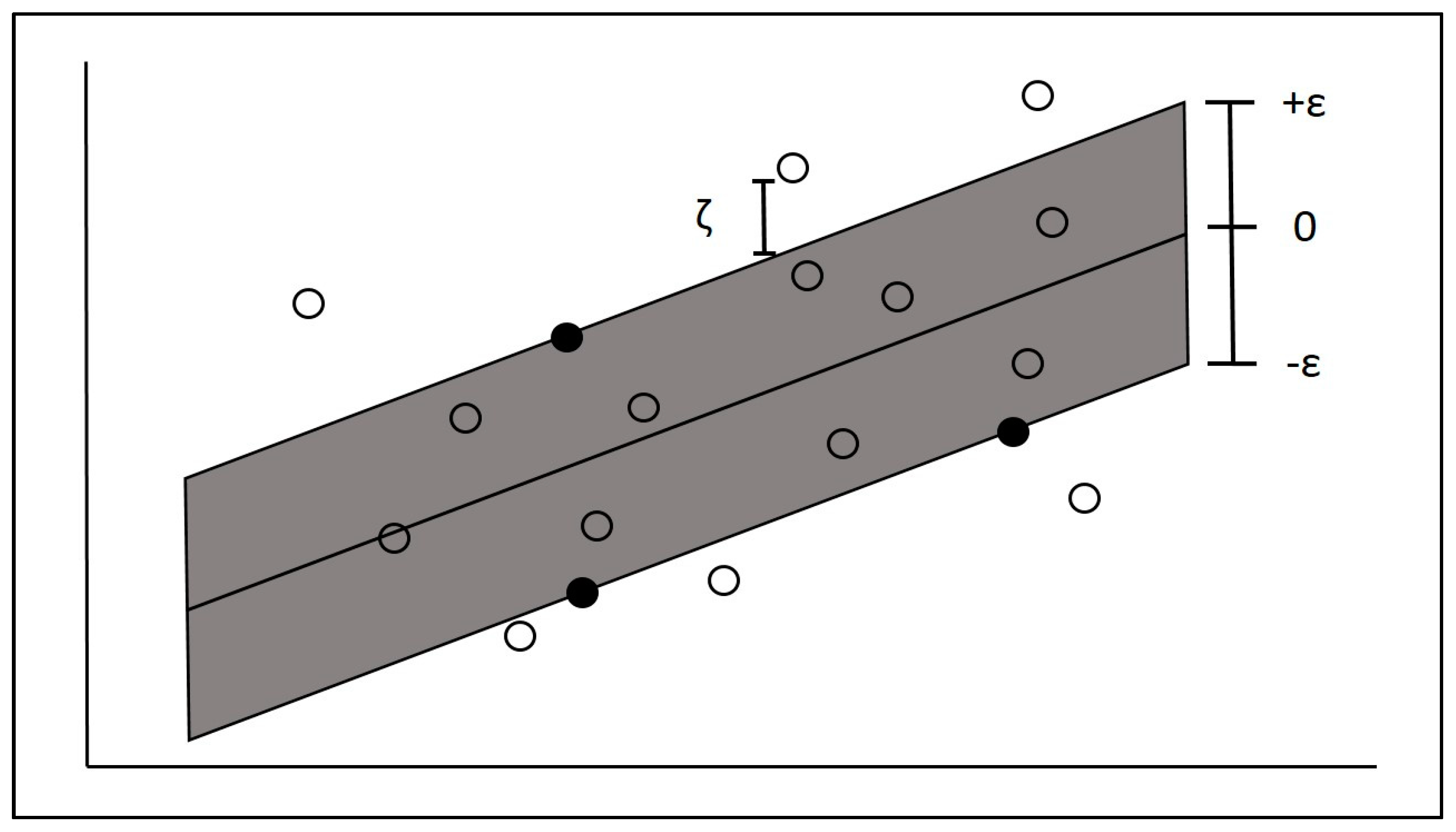
The basic concept of SVR is the creation of a tolerance band of width ε around the regression line. All the points in our dataset are expected to lie inside this tolerance band; in mathematics, this means that we tolerate all the predicted values to fall within a
of the true values. The objective of SVR is to minimize the coefficients through the l2-norm of the coefficient vector. The errors are handled in the constraints, where we restrain the absolute error to the maximum error ε. When training the model, the ε is tuned according to the desired model accuracy. The objective function and constraints are:
The presented model is an unrealistic model since it cannot tolerate any error outside the ε-tolerance band. To allow larger than ε errors, we add the slack parameter
in our model as follows:
The constraint
allows points to lie out of the band, though the addition of the slack parameter
in the objective function ensures that we want them to remain as close to the band as possible.
Figure 3 gives an illustration of the SVR paradigm with slack variables.
The points in the margin of the ε-tolerance zone are called Support Vectors and they define the position of the regression line.
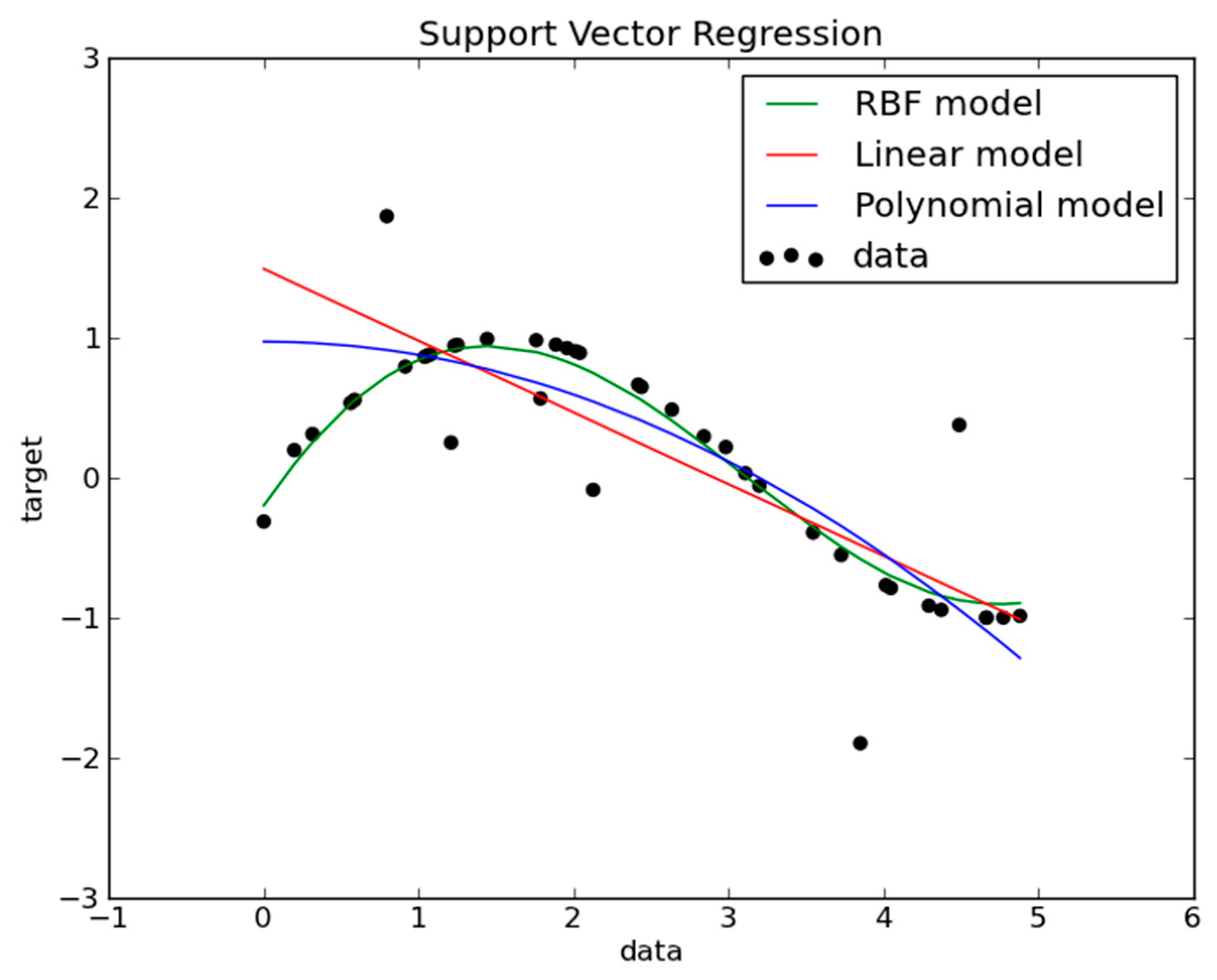
When the problem at hand cannot be treated using a linear classifier, then we use the kernel trick to change the dimensionality of the space where the optimization is performed during the training. The data points from the initial variable space of
n-dimensions (in our illustrated example it is two dimensions) are projected into a higher dimension space, called the feature space, where the regression hyperplane creates the acceptable error; see
Figure 4. When the kernel function is non-linear, the produced SVR model is also non-linear.
4.2. Decision Trees
Decision Trees are a supervised machine learning algorithm that is used for both classification and regression tasks. It works by recursively partitioning the data based on the most informative features. They are flowchart-like top-down structures of nodes and branches; see
Figure 5. In regression tasks, the decision tree predicts the value of the target variable by averaging the values of the training data points that fall into the same leaf node.
The top node is the root node representing the complete dataset. The decision nodes are if statements on one variable of the dataset. The two branches below each decision node split the dataset into two subsets: a subset where the decision node is true and a subset where the decision node is false. The nodes that do not split any further are called leaf (or terminal) nodes and depict the final outcomes of the decision-making process (in our case, a value for the regression procedure).
4.3. Random Forests
The Random Forests model explores the idea of many decision trees combined though a bootstrapping–aggregating algorithm, called bagging; see
Figure 6. In each tree, a different randomly selected replacement subsample equal to the size of the initial dataset is used and a randomly selected subset of the initial independent variables is used for training the tree. The model’s ability to perform in unknown data is estimated using the observations not selected in the training step (this data part is often called out-of-bag in ML terminology). Thus, in the Random Forests algorithmic procedure, a stochastic process is implemented in choosing both the observations used for training (rows of the data matrix) and the independent variables (columns of the data matrix). In regression tasks, the prediction is made by calculating the average value of the target variable from the data points within every leaf node. In our experiments, we used two strategies: Random Forests with unlimited splits (partitionings) of the dataset and Random Forests with limited splits (8 splits).
4.4. Boosting
Boosting is based on the idea of accumulating sequentially weak learners, each correcting its predecessors. The weak learners in our case are shallow decision trees, i.e., decision trees with few partitions of the dataset. Each added decision tree corrects the regression and improves the performance of the overall model. The combination of all the shallow decision trees constructs the boosted model (see
Figure 7). In our experiments, we used the XGBoost algorithm to perform the boosting procedure.
4.5. Forecast Evaluation
All models were evaluated using the Mean Absolute Percentage Error metric, defined as:
where
and
are the actual and the forecasted values of the target variable, respectively, and
is the sample size. The MAPE metric measures the mean absolute distance between the actual and the forecasted values in percentages.
5. Results and Discussion
We trained an arsenal of ML-based models, including Support Vector Machines, Random Forests, and XGBoost, and tested it in two setups: (a) one using all the independent variables of our dataset, and (b) one using only the top-15 most informative independent variables
1 (
Table 2). From these results we can see that all weather variables sum up to 32.96% relevance, while all car sales variables add to 30.55%. Thus, of the 15 most important variables, a total of 63.51% relevance is attributed to either the weather or car sales.
For each model, we calculated the MAPE for the training and testing subsets, and for the out-of-sample part. Nonetheless, due to the small size of our dataset (48 observations comprises a small dataset even for the selected methodologies), we choose to evaluate the performance of every model using the MAPE metric on the whole dataset. In
Table 3, we present the results from all the subsets and the full dataset.
Overall, the best model was the Random Forests model with limited depth, which was fed with the top-15 most relevant variables and reached a MAPE of 18.24%. The second-best model was the XGBoost with the top-15 most relevant variables, which reached a MAPE of 19.56%. In
Figure 8, we show the graphical representation of the actual and the forecasted values from the best model.
It is easy to verify that in most cases the forecasted values are visually close to the actual ones. Indeed, the peaks and troughs of both time series in
Figure 8 coincide. Despite the model’s failure to detect the peaks during the second quarter of 2011 and the third quarter of 2017, the mean absolute percentage error (MAPE) between 2011 and 2016 was calculated to be 7.6%.
The analysis performed indicates that the five variables with the most relevance, or, in other words, the best predictors of insurance claims, are: the number of new cars with a time lag of 3 quarters and 1 quarter, respectively, followed by the minimum temperature recorded at the Elefsina station 3 quarters ago, the number of new cars 2 quarters ago, and the moving average of new car registrations. The next five variables with respect to forecasting importance are: the minimum temperatures at the Tatoi station 1 quarter ago, the minimum temperatures at the Elefsina station 2 quarters ago as well as the mean temperatures at Elefsina 3 quarters ago, the rain at Spata station 4 quarters ago, and the mean temperature at Elefsina 1 quarter ago. The last set of five variables among the top 15 predictors are the mean insurance claims per car 4 quarters ago, the mean insurance claims per car 3 quarters ago, the minimum temperature in Elefsina 1 quarter ago, the moving average of the mean insurance claims, and the minimum temperature in Spata 3 quarters ago.
According to these results, the registration of new cars appears to be one of the most significant predictors of insurance claims. This may be attributed to the fact that as more new cars circulate, the number of accidents increases and thus the total claims cost increases, yielding a higher mean claims amount per insured vehicle in the motor portfolio under investigation. The time lag (of one to three quarters) is possibly justified, as drivers tend to be more careful when their car is brand new, and they stop paying that much attention as their car ages.
Furthermore, the lowest temperature can impact the overall claims expense because when such a temperature is recorded, the overall claims expense increases (potentially influenced by the number of accidents), leading to a consistently higher mean claims amount per insured vehicle in our motor portfolio. The time lag seems to be consistent with the new car time lag. The same is observed for the mean temperature and the rain, which is most likely due to a similar reason.
Finally, the mean insurance claims (per car with a time lag or moving average) affect the mean insurance claims per vehicle, but with a lower predictive capacity, indicating that the historical experience of the average claim amount is important for the determination of the current average claim amount. Indeed, one can expect that for a rather mature motor insurance portfolio, past claims can be (and are in practice) used to project future claims.
One potential explanation for the time lag is that claims are not immediately reported or paid. Consequently, they may be paid later in time. Moreover, when there are bodily injuries, the total claims amount increases and the time period over which the claim is paid is longer.
According to
Table 2, which shows the top-15 variables in terms of importance, the weather variables (Min Temp Elefsina t − 3, Min Temp Tatoi t − 1, Min Temp Elefsina t − 2, Mean Temp Elefsina t − 3, Rain Spata t − 4, Mean Temp Elefsina t − 1, Min Temp Elefsina t − 1, and Min Temp Spata t − 3) have a significance of 32.96%, while the car sales variables (New Cars t − 3, New Cars t − 1, New Cars t − 2, and Moving Average New Cars) contribute 30.55%. Therefore, out of all the variables available, the 12 variables mentioned above measure a combined relevance of 63.51%, which is attributed either to the weather or to car sales. Additionally, there is a positive correlation between the total amount of insurance claims and the Greek real GDP. The relevant Pearson correlation coefficient is
, which is highly significant. The high correlation between the total insurance claims and the real GDP may be due to the fact that the increasing economic activity leads to increased transportation needs both in distance and time travelled. Thus, firms are in need of being supplied by more raw materials; more goods are produced, traded, and distributed to the retail stores; consumers and employees spend more time driving to shopping centers and to work; traffic jams are more frequent; and, also, usually more people use their private vehicles instead of public mass transportation when their income increases.
Overall, given the limited dataset that was supplied to us for this study, the algorithms employed seem to produce quite satisfactory results in terms of the MAPE that approximately ranges between 18% to 25%. Moreover, the Random Forests limited depth algorithm exhibits the best performance, especially during the time period from 2011 to 2016; one can see that the distance between the peaks and troughs in that period is comparatively smaller. This indicates that the models employed can be quite reliable when used by insurers for forecasting their motor insurance claims evolution.
6. Conclusions and Further Research
In this paper, we offer an innovative approach for insurance claims forecasting. The innovations of our approach are threefold: (a) we introduce two novel arrays of variables, i.e., weather conditions and car sales; (b) we managed to get the permission to use a proprietary dataset from an actual insurance company; and (c) we employ an arsenal of Machine Learning (ML) algorithms (Support Vector Machines, Decision Trees, Random Forests, and Boosting). We forecast the mean insurance claims amount per insured car per quarter and also identify the variables that are the most relevant in this forecast. The results show that the three most relevant variables are the new car sales with a 3-year and 1-year lag and the minimum temperature of Elefsina (one of the weather stations in Athens) with a 3-year lag. Random Forests limited depth and XGboost, which were run on the top-15 variables in terms of relevance, are the best performers. Overall, weather variables sum up to 32.96% relevance, and car sales variables sum up to 30.55%.
Insurance companies may take advantage of these results when they attempt to forecast their future claims evolution by using weather conditions and new car sales as variables that affect claims. Furthermore, they can employ ML techniques when performing these forecasts, instead of the traditional actuarial approaches, as they seem to deliver quite reliable results.
Future research venues pertain to the forecasting of the claims frequency, as well as a deeper analysis of the findings of this paper, potentially using larger motor portfolios to train more accurate models, better test the validity of the results, and provide more thorough interpretations of the results.
As a next step, future research incorporates the simultaneous study of the new sets of variables reflecting weather conditions and car sales and the traditional set of variables capturing vehicle characteristics (such as type of vehicle—e.g., passenger car, truck, motorcycle, etc.; vehicle use—e.g., private car, commercial car, etc.; horsepower; weight; car make and model; manufacturing year; etc.) and driver characteristics (such as age, gender, driving experience, lifestyle, marital status, etc.).


