1. Introduction and Literature Review
1.1. Introduction
Option pricing is an important research field within financial markets and has attracted a considerable amount of attention from both academics and practitioners for a long time. The American option, a common financial derivative, requires accurate and quick pricing solutions, which are critical for the stability and development of the financial market. With the significant advancements in computational technologies, computerized computational methods have been widely used for optimal pricing. Among these, least squares Monte Carlo (LSMC), a relatively new and effective technology, has been utilized to solve the American option pricing problem. In this paper, we discuss the application of distributed computing technology to enhance the LSMC method in terms of American option pricing.
Currently, there are several researchers (
Weigel 2018) who have used the method of parallel computing to improve the LSMC method, but, for the first time, we use this paper to discuss distributed computing technology to improve the LSMC method. In parallel computing, the computer’s memory is shared, but, in distributed computing, the memory is separated so that it can be referenced as a single shared space that runs independently. The method of distributed computing has several advantages over parallel computing. Firstly, distributed computing can reduce the overall computational complexity of the algorithm by using the “divide and conquer” method for the total computational complexity. The sum from each computer node is less than the original total computational complexity executed on the single note without using distributed computing. This advantage was supported by the mathematical theory of distributed regression (
Dobriban and Sheng 2021). Secondly, compared with the traditional parallel least squares regression, distributed regression does not require complicated matrix transformation techniques. Thirdly, distributed computing can help protect the privacy and security of the given data. These data can be stored in the original locations of the distributed system, and moving the data around will not be required. Lastly, the LSMC method itself is suitable to be computed distributively because the paths can be simulated and regressed separately.
The goal of this paper is to show through research how distributed computing, especially distributed regression technology, can be used to improve the LSMC method regarding the efficiency and accuracy of American option pricing. Our paper provides a new solution to the financial market, and we expect it can provide innovation and progress in the field of American option pricing.
The rest of the paper is organized as follows. In
Section 2, we discuss the generic Monte Carlo simulation for American option pricing and its computational complexity. Comparatively,
Section 3 introduces the least squares Monte Carlo simulation in which we discuss its advantages and limitations for option pricing. In
Section 4, we discuss distributed regression to the LSMC method to further speed up its computational process.
Section 5 provides detailed computational complexity comparisons of other option pricing approaches in which we rank which ones are the most accurate and fast. Next,
Section 6 aims to further validate the distributed LSMC by performing an experiment using PySpark 3.3.1 and Python 3.9.7. Finally, we conclude the paper in
Section 7.
1.2. Literature Review
The Black–Scholes model was developed by
Black and Scholes (
1973) to calculate the price of European options using a differential equation with various variables, such as the current stock price, strike price, risk-free rate, volatility, and time to maturity or expiration. Although the Black–Scholes model can provide an analytical solution for European options, it is not applicable to American options due to their added complexity as they can be exercised before the expiration date. For American option pricing, numerical methods such as Monte Carlo simulation and the binomial tree model are typically used to estimate the option value.
The binomial tree model, originally introduced by by
Cox et al. (
1979), was developed as a visual illustration of the Black-Scholes model by the three financial educators. The binomial tree model relies upon the same variables as the Black–Scholes model to create an array of pathways to view specific stages of an option price. The option price will fluctuate up or down depending on the interest or discounted rate, length of time, and volatility that the option contract is subject to. With the increase in the time steps, the number of nodes in the binomial tree increases exponentially, which makes the computational complexity significantly higher (
Dai and Lyuu 2010). The computing needs for a large number of nodes could result in too much time in computing, especially when high-accuracy pricing is required.
Tilley (
1993) first proposed using the Monte Carlo method for American option pricing, but this solution has not seen widespread use due to issues such as its complexity. The breakthrough in this area came with
Longstaff and Schwartz (
2001), who introduced the least squares Monte Carlo (LSMC) method to ascertain the optimal relationship between the continuous value of the derivative security and the value of the relevant variable at each moment. They then determined whether the option should be executed in advance at a specific moment. Currently, the LSMC method has become the standard method for pricing American options. This method estimates the option price by generating various paths that allow for the observation of multiple price points and the determination of the optimal point at which to exercise the option. The paths are determined by a range of variables, such as stock price, option price, time to maturity, risk-free rate, frequency, dividends, and volatility. LSMC has many applications; for instance, it has become a popular proxy technique for reducing the computational complexity of Solvency Capital Requirement (SCR) under the Solvency II framework (
Bauer et al. 2010;
Krah et al. 2018). Proxy techniques are mathematical approximation methods used to estimate a quantity of interest when it is too difficult to measure directly. Under fairly general conditions,
Clément et al. (
2002) proved the almost sure convergence of the LSMC algorithm. They also determined the rate of convergence of approximation and proved that its normalized error is asymptotically Gaussian.
Haugh and Kogan (
2004) developed a dual method Monte Carlo for pricing American options. This method constructs upper and lower bounds on the true price of the option using any approximation to the option price. Numerical results suggest that this approach can be successfully applied to problems of practical interest.
In the field of pricing American options using machine learning,
Goudenège et al. (
2019) proposed an efficient method to compute the price of multi-asset American options based on machine learning, Monte Carlo simulations, and the variance reduction technique.
Chen and Wan (
2021) proposed a deep neural network framework for computing prices and deltas of American options in high dimensions.
Datta (
1985) proposed an effective parallel algorithm that uses matrix decomposition techniques such as QR decomposition or Cholesky decomposition.
Chen et al. (
2015) accelerated the least squares Monte Carlo method with parallel computing.
Zhang et al. (
2015) proposed a “divide and conquer” type of distributed regression algorithm.
Dobriban and Sheng (
2021) provide a mathematical theory of distributed regression. However, there is no research studying the application of distributed computing in LSMC, an area this paper intends to explore.
2. Generic Monte Carlo for American Option Pricing
Consider an American put option, assuming that
T is the expiration time, where
is the optimal exercise time, and
is the asset price at time
t. The price of the American put option at time 0 is given by
where
is the risk neutral measure.
To perform a Monte Carlo simulation, we assume that the stochastic process
, which is the asset price, follows geometric Brownian motion, so it satisfies the following stochastic differential equation (SDE):
where
r is the drift or risk-free interest rate of the asset,
is the volatility of the asset, and
z is a Brownian motion. According to Itô’s formula, (
2) derives
Using the discretization method, we divide the whole time interval
to
N sub-intervals:
, and then we can derive the following approximate recurrence formula from (
3):
where
follows the standard normal distribution. From (
4), we can further derive the following formula for
:
After simulating M paths, denoted as , we obtain an matrix representing the price paths.
The intrinsic value or the early exercise payoff for an American put option of path
j at time
i is
when the asset price is
. The option price of path
j at time
i is
Computing the continuation value
in Formula (
6) of the generic Monte Carlo requires a full revaluation of the option price at each time step with a new set of random paths. This essentially represents a “nested Monte Carlo” simulation, which is extremely time- and memory-consuming.
The computational complexity of the generic Monte Carlo simulation for formula (
6) is
, where
is a positive integer and
N is the number of sub-intervals.
3. LSMC
3.1. Introduction of LSMC
The LSMC method originates from non-parametric regression. The goal of non-parametric regression in statistics is to estimate the conditional expectations:
, where
and
are the response variable (stock price) and covariate (continuation value), respectively. In statistical problems, observations of
and
are accessible, and non-parametric regression methods can estimate the function
based on the samples. It is called non-parametric regression because the form of the function
requires minimal assumptions and can be a general non-linear function. Geometric Brownian motion can also be used to simulate future stock prices. The LSMC simulation is similar to a traditional model in that it involves the allocation of the remaining time of an option’s expiration. A random sample of the asset price path is generated, and the expected return of the option is compared with the expected return of the underlying asset. If the exercise value exceeds the expected holding value, it is the ideal strategy to sell the option immediately. Least squares regression is used for the approximation of the continuation values in which each continuation value is a function of the stock price. We can denote the continuation value as follows:
The generic (nested) Monte Carlo method of option pricing applies the payoff function and takes the discounted expectation of those paths’ payouts to obtain the option price. However, computing continuation values at future time points becomes less straightforward with this approach. The generic Monte Carlo method tends to be inefficient when dealing with large sets of constraints. One could complete this with nested simulations, but this would not be practical since the computational complexity , where C is the number of simulated scenarios at each time point), is so large that we need to introduce the LSMC algorithm to reduce the running time of the generic MC.
To improve the efficiency of the nested Monte Carlo simulation, the LSMC method was first proposed by
Longstaff and Schwartz (
2001). This method involves simulating the paths and then working backward in time to estimate the continuation values through least squares regression. The fitted regression curve can be used to average the errors, producing a more accurate solution through a faster process.
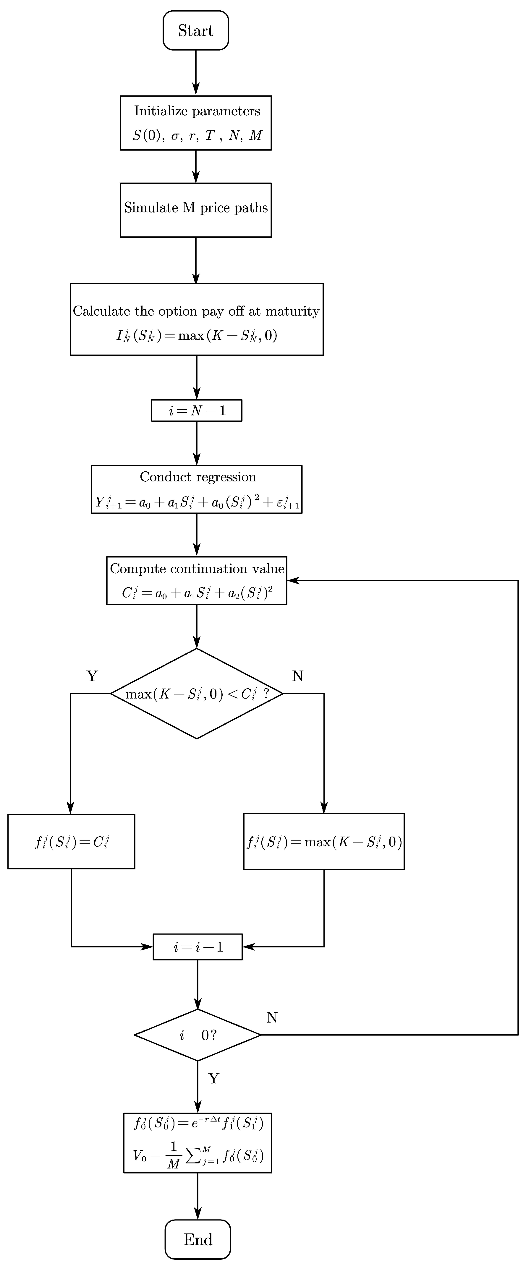
3.2. Algorithm Steps of LSMC
- Step 1
Initialization and simulation of asset price paths.
Initialize the parameters of the problem, such as the initial underlying asset price
, volatility
, risk-free interest rate
r, time to maturity
T, number of time steps
N, and the number of simulated patterns
M. Use geometric Brownian motion to simulate the
M price paths of the asset from time
to
with N time steps. Given the asset price at the time step
, the asset price at the
ith time step can be derived using the following equation:
where
is a standard normal random variable, and
j is the path index.
- Step 2
Valuatiton of the option at maturity.
Calculate the option payoff at maturity for each simulated path. For an American put option, that payoff is
where
K is the strike price.
- Step 3
Backward induction.
Starting from time step and going backward to , perform the following steps:
Regression: Conduct the least square regression for the continuation value at time
using the basis functions, which take the underlying asset price at time
i as input. The regression model is
where
is the discounted continuation value of the option at time
.
Decide on continuation value or early exercise: Compute the continuation value and compare it with the early exercise payoff. If the latter is larger, then set ; otherwise, set .
- Step 4
Estimation of the option price.
Once we reach time
, the estimated option price is the average of the discounted option value
over the
M paths (
Longstaff and Schwartz 2001):
Figure 1 shows the algorithm flow chart of LSMC.
3.3. Convergence and Computational Efficiency of LSMC
The effectiveness of the LSMC algorithm is evaluated from two aspects: convergence and computational efficiency. They mainly depend on the number of odd functions
K, the number of discrete time points
N, the number of sample paths
M, and the method used to generate the simulated random numbers. Regarding the convergence of the LSMC algorithm, Longstaff and Schwartz proved that, if the number of sample paths M tends to infinity, as long as the number of basis functions is large enough, the simulated option value will converge to the actual option value. In addition, a very important feature of the LSMC algorithm is its excellent computational efficiency. Compared with the generic Monte Carlo, the computational efficiency of the algorithm is more than 600 times more efficient (
Tian and Benkrid 2009).
3.4. Limitations of LSMC
While LSMC simulation holds the benefit of accuracy, it is subject to some criticism and has limitations. Its performance is possibly affected by the choice in regressors. The number of regressors in the LSMC model increases exponentially when there are multiple risk factors and higher degree terms included in the basis function. This can dramatically slow the computation. Also, the LSMC method is often unsatisfactory in situations involving non-linearity. In fact, the original LSMC method’s performance depends on the choice of the appropriate basis variables and their associated functions, which requires the correct selection of basis functions to ensure the accuracy of estimation as well as the most accurate number of simulation paths. However, a polynomial as the base function provides an accurate estimation of the option price regardless.
Financial institutes face exposure to multiple risk factors, such as market prices of financial securities, long-term interest rates, exchange rates, and prices inflation, etc. (
Lin et al. 2018). When the LSMC model is applied to financial practice, usually, dozens of risk factors are used as regressors to estimate the conditional expectation in this model. When multiple risk factors are included in the LSMC model, the number of regressors in the regression step increases exponentially, which would make the computation slow. On the other hand, the degree could be very high, and the relationship between the independent variable and the dependent variable may be complex and non-linear when using machine learning. When there is complex and non-linear interaction between the independent and dependent variables, using the higher-degree regressors can help to capture the complexity in these relationships. The number of regressors can be determined by the following formula, where
D is the degree of the regression equation and
R is the number of risk factors:
Table 1 provides an illustrative example of the relationship between the number of regressors with different degrees and the number of risk factors based on Formula (
12).
4. Distributed LSMC
4.1. Distributed Regression
To further speed up LSMC, we introduce distributed regression and MapReduce to LSMC. In 2015,
Zhang et al. (
2015) proposed a simple yet powerful distributed regression algorithm. This algorithm divides the entire dataset into multiple subsets, applies regression to each subset data, and then averages the results. We can distribute all the paths in LSMC across multiple computing nodes and average the results computed from all the nodes to obtain the final price of the option. Assume M is the number of paths, N is the number of time steps, K is the number of basis functions used in the regression, and m is the number of distributed computing cores. This process can be implemented using MapReduce, which is a divide and conquer method, and this process is efficient with computational complexity between
and
compared with ordinary regression LSMC with computational complexity
.
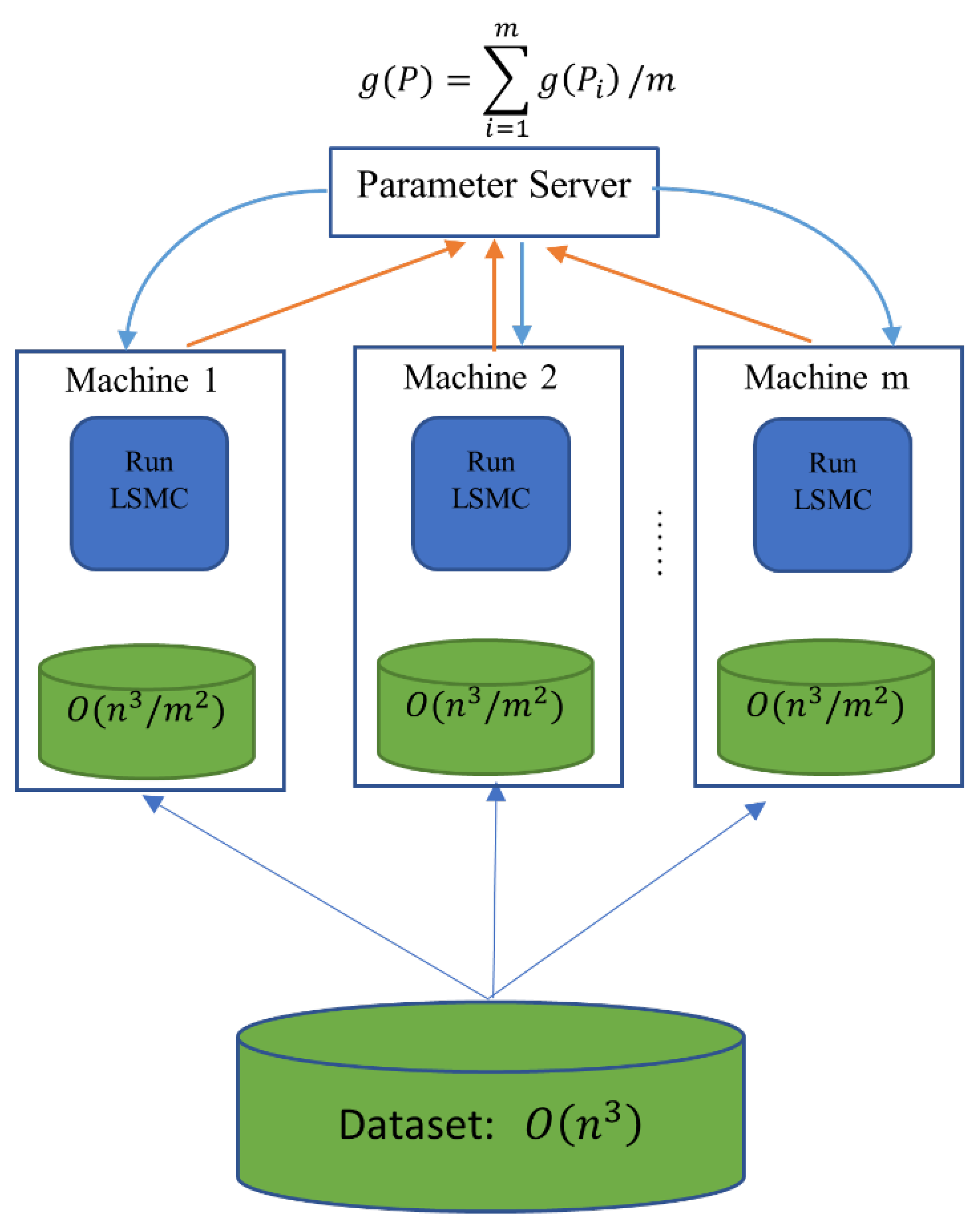
The idea of distributed LSMC is illustrated in
Figure 2. The entire dataset
P is partitioned into
m subsets (usually of equal size), and these subsets are labeled as
and then distributed to each machine. The parameter server collects the estimated option price
obtained by machine
i from the subset,
, and then the parameter server computes their average value
, which yields the final estimated option price.
The primary advantage of employing distributed computing in LSMC is its ability to significantly reduce the total computational complexity of the algorithm by distributing the workload across multiple nodes, which is called the divide and conquer method. This can lead to faster computation times and improved scalability, allowing for the efficient pricing of American options and even large portfolios of derivatives.
Additionally, distributed computing can provide fault tolerance and increased reliability by allowing for redundant computations and reducing the risk of system failures or crashes.
Finally, distributed computing can protect data privacy by using data fragmentation, secure communication protocol, and other technologies such as encryption. By breaking the data into smaller subsets and distributing them into multiple computers, each computer has its own security measures. By doing this, it is more difficult for hackers to access whole datasets because they must compromise multiple systems simultaneously.
4.2. Validation of Distributed LSMC
Inspired by distributed regression, we propose the distributed LSMC to reduce the runtime of LSMC.
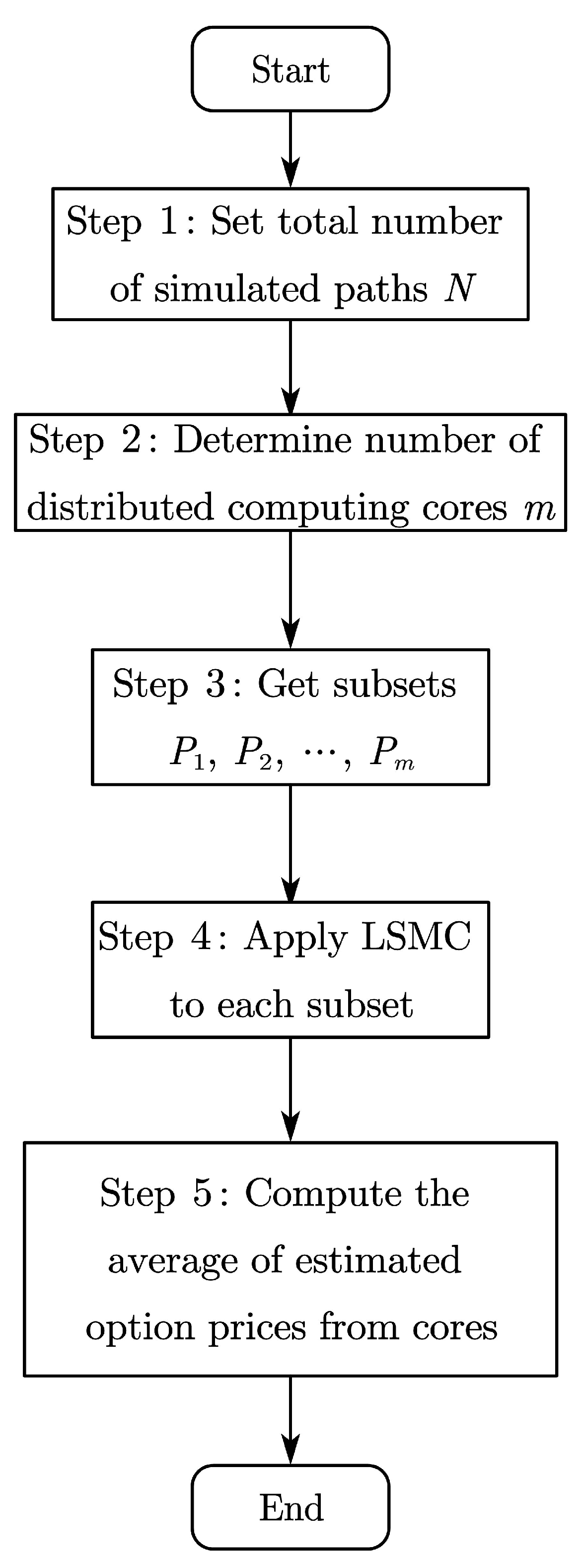
Figure 3 shows the flow chart of the distributed LSMC as described in Algorithm 1.
In the following paragraphs, we will discuss the validity of the proposed distributed LSMC algorithm. We will focus on explaining why this algorithm can obtain the same result as the traditional LSMC. Firstly, the LSMC method, like other Monte Carlo methods, is based on the Law of Large Numbers (
Graham et al. 2013). As the sample size increases, the sample average converges to the population expectation. Therefore, if we simulate the price paths and calculate the payoff of the option using LSMC independently on each computer node, we can expect the estimated value from each node will converge to the same result with enough simulated paths. Secondly, in our proposed distributed algorithm, each path on the distributed computer node is mutually independent and the asset returns follow the same probability distribution. Therefore, when we average these independently estimated option payoffs, we can obtain a stable and accurate estimation of the actual option price.
| Algorithm 1: Algorithm of Distribution LSMC |
- 1
Step 1: Set the total number of simulated paths N. - 2
Step 2: Determine the number of distributed computing cores m. - 3
Step 3: Equally divide the N simulated paths into m subsets, each containing paths. Label these subsets as . - 4
Step 4: On each computing core i, independently generate path subset and apply the LSMC algorithm to to obtain the estimated option price . In this step, the LSMC algorithm used on each core is the same as the conventional LSMC method. - 5
Step 5: Compute the average of all the estimated option prices from the computing cores as the final estimated option price: .
|
Theorem 1. The expected result from the distributed LSMC method is identical to the expected result from the traditional LSMC method, i.e., Proof. LHS:
is the expectation of the option payoff calculated by LSMC over all paths; according to
Longstaff and Schwartz (
2001), this equals the true option price
V.
RHS: Note that each is an independent subset of all paths; hence, the expected option price by LSMC for each subset is also V. Therefore,
Hence, □
This theorem proved that both methods produce the same expected results. Also, because both the traditional and distributed LSMC will converge to their expected estimation of the option price, they will converge to the same results. Therefore, Theorem 1 proved the equivalence of the results produced by both methods.
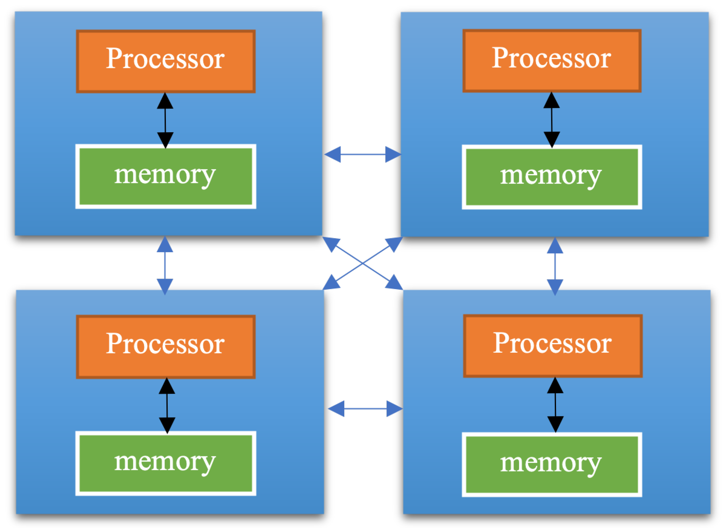
Several researchers have applied parallel regression in LSMC. Parallel computing for regression problems often involves more complicated matrix computation. Especially in the least square linear regression, an effective parallel algorithm is using matrix decomposition techniques such as QR decomposition or Cholesky decomposition (
Datta 1985). The distributed LSMC has advantages over the parallel LSMC in terms of computational complexity and scalability. By avoiding the complex matrix computation in the parallel LSMC, the distributed LSMC reduces the total computational complexity by partitioning the data into smaller subsets. In addition, this strategy naturally fits the architecture of cloud computing, which is built on distributed computing technologies. With enough cloud computing resources, we can greatly reduce the computing time required and provide advantages in application environments where efficiency and scalability are critical (
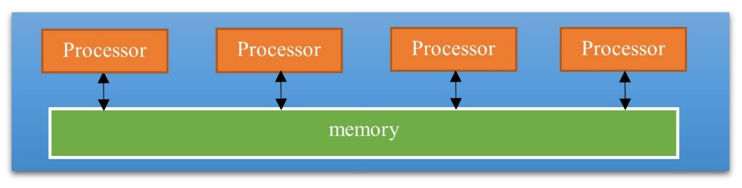
Leopold 2001). It is essential to distinguish between these two approaches (
Riesen et al. 1998). A parallel computing system consists of multiple processors that communicate with each other using a shared memory, as shown in
Figure 4, whereas a distributed computing system contains multiple processors connected by a communication network, as shown in
Figure 5. The parallel regression requires complex matrix transformations, while the distributed LSMC method we proposed here does not require that (
Datta 1985).
5. Computational Complexity Comparison
Computational complexity is a branch of theoretical computer science that focuses on the time and space complexity of algorithms. Big
O notation is often used to compare different algorithms and to choose the most efficient algorithm for a given problem (
Devi et al. 2011).
The following is the complexity analysis of some American options pricing approaches.
Assume M is the number of paths, N is the number of time steps, K is the number of basis functions used in the least squares regression, m is the number of distributed computing cores, and represents the number of scenarios corresponding to each scenario at the previous time step.
For the binomial tree approach, the computational complexity is . This is because the tree has time steps N, and, at time , there are nodes. Therefore, the total number of nodes in the binomial tree is , so the computational complexity is if dismissing other terms with smaller power.
For the generic Monte Carlo (also known as nested Monte Carlo), assume represents the number of considered possible scenarios corresponding to each scenario at the previous time step (except from those of the last level), and N represents time steps. We only focus on the number of scenarios in the last level, which is . Thus, the computational complexity is .
The ternary tree is a special case of the generic Monte Carlo method, where ; therefore, the computational complexity is .
In the LSMC method, the regression at each time level involves the building of a square and symmetric matrix via the system of normal equations. The least squares solution can be computed using efficient methods such as Cholesky factorization, which has a computational complexity of
. However, the construction of the matrix
A has complexity
(
Stothers 2010) based on the complexity of matrix multiplication. In typical data fitting problems,
, and, hence, the overall complexity of the normal equations method (
Herzberger 1949) is
. Considering that there are N time steps, the computational complexity of LSMC is
.
The distributed LSMC involves the simulation of the price paths, least squares regression for the continuation value, and comparison between the early exercise value and the continuation value, etc. In the regression step, the distributed LSMC can reduce the overall computational complexity to but does not change the complexity of other steps. Therefore, the computational complexity of the distributed LSMC will be lower than the traditional LSMC but higher than the pure distributed regression .
We can rank the computational complexities of these methods as
. We put these results in
Table 2.
6. Experiment: Result of Distributed Regression Method for LSMC
In this chapter, we aim to conduct a series of computing experiments for the distributed LSMC we have proposed. We will evaluate the computing speed and accuracy of the distributed LSMC vs the traditional LSMC. The main goal of this comparison research is to validate the theory we derived, that these two methods would produce equivalent and very close results.
When it comes to computing speed, we anticipate that the distributed LSMC method provides a significant performance improvement. This anticipation of the efficiency increase comes from the intrinsic advantage of distributed computing, which uses the computing resources of multiple machines to reduce the total computing time. On the other hand, the distributed LSMC can reduce the total computational complexity, which results in shorter computing time required. This chapter will discuss the experimental study results to support these statements.
Our experiment was carried out on Google CoLab equipped with the following hardware specifications:
There are two popular frameworks to implement distributed computing: Hadoop and Spark. The bottleneck of the Hadoop MapReduce is unnecessary data reading and writing, and this is the main improvement in Spark. Specifically, Spark continues the design idea of Hadoop: the calculation of data is also divided into two types: Map and Reduce. However, the difference is that a Spark task does not only include a Map and a Reduce but consists of a series of Maps and Reduces. In this way, the intermediate results of the calculation can be efficiently transferred to the next calculation step to improve the performance of the algorithm (
Fu et al. 2016). Although the improvement in Spark seems to be small, the experimental results show that its algorithm performance is 10–100 times higher than that of Hadoop (
Mostafaeipour et al. 2021).
Because of the advantages of Spark, we use PySpark 3.3.1 and Python 3.9.7 for distributed LSMC implementation.
The following is detailed information about the American option example we are going to price.
Initial underlying asset price: = USD 100.
Strike Price: K = USD 101, K = USD 200.
Time to expiration: “days”. This is the length of time during which the American option contract is valid.
Annualized interest rate: .
Annualized volatility of underlying asset return: .
Dividends: . Assume no dividend is paid during the life of the option contract.
The benchmark values for the above American options, with strike prices of K = USD 101 and USD 200, are USD 2.455145310460293 and USD 100, respectively. They will be used as the benchmark to compare our computing results.
Please refer to
Table 3 and
Table 4 for our speed experiment results. We used two computer cores on Google CoLab and tried different numbers of paths ranging from 1 million to 10 million. All the computations were performed in double precision to ensure a high degree of accuracy when comparing the small errors. From these results, we found that the distributed LSMC is consistently faster than the traditional LSMC. In addition, with the number of paths increasing, the percentage of time the LSMC method saves also increases. For instance, in
Table 3, when considering 1 million paths, the distributed LSMC is about 65% faster than the traditional LSMC. With 10 million paths, the improvement becomes more significant, where the distributed LSMC is nearly three times faster. This phenomenon could be due to the startup time by the PySpark when initiating distributed computing. As the number of computing tasks and the amount of data being processed increase, this fixed amount of starting time becomes a smaller fraction of the total computing time. Therefore, as the simulated paths increase, the relative speed advantage of the distributed LSMC becomes more obvious. These results confirmed the advantages of the distributed LSMC method in large-scale computing tasks.
The accuracy of our distributed LSMC compared with traditional LSMC is listed in
Table 5 and
Table 6. The second and third columns of these tables show the pricing results of two algorithms with different numbers of simulated paths. The last two columns are percentage errors of the pricing results by comparing two algorithms with the actual option price. This result shows that the distributed LSMC can achieve comparable pricing accuracy to the traditional LSMC. As the number of paths increases, both methods produce more accurate results. Thus, we conclude that our distributed LSMC can achieve faster computing speed than the traditional LSMC without sacrificing accuracy.
7. Conclusions
This paper has explored the application of distributed computing technology in enhancing the LSMC method for American option pricing. Option pricing is a critical area of research in the financial market, and the efficiency and accuracy of pricing solutions play a significant role in the stability and development of the market. While computational techniques, including parallel computing, have been widely utilized to optimize pricing algorithms, this paper stands out as the first to investigate the potential of distributed computing technology for LSMC enhancement in American option pricing.
Compared to parallel computing, distributed computing offers several advantages. By employing a “divide and conquer” approach, it reduces computational complexity, enabling faster and more efficient calculations. Moreover, the distributed computing approach eliminates the need for complicated matrix transformations and enhances data privacy and security. These advantages make distributed computing a suitable and promising technique for LSMC in American option pricing. The LSMC method itself aligns well with the distributed computing paradigm since price paths can be simulated and regressed separately.
To validate the correctness of the distributed LSMC algorithm we proposed, we proved the equivalency of distributed and traditional LSMC methods in terms of pricing expectations in probability theory. In addition, we analyzed the computational complexity of some American option pricing methods: binomial tree, ternary tree, generic Monte Carlo, traditional LSMC, and the distributed LSMC proposed in this paper. The distributed LSMC has the least computational complexity.
The primary objective of this research was to showcase how distributed computing can significantly improve the accuracy and efficiency of LSMC in American option pricing. For this reason, we conducted numerical experiments for both the traditional and distributed LSMC, which verified the accuracy and efficiency of the distributed LSMC.
Other than the application in American option pricing, the distributed LSMC method proposed in this paper also has broad application in the insurance industry. This method works for the insurance products that contain the American option or those similar to the American option. For instance, the variable annuity includes the embedded American style options for the policyholder, and its fair market value depends on the performance of the underlying investment portfolio. The distributed LSMC can provide efficient and accurate pricing results for these types of products that are complex and path-dependent.
However, there are certain limitations of the study worth mentioning. Firstly, we only explored polynomial functions as base functions with degree 2, whereas there are many other types of base functions available, such as triangle functions, spline functions, and wavelet functions. Further, the degree could be increased. Optimizing the choosing of base function and degree could improve the performance of the algorithm. Secondly, we conducted the experiment using only two CPU cores, without increasing the number of cores. Thirdly, distributed computing involves communication between different computing nodes, which can introduce overhead due to data transfer and synchronization. The increased communication overhead can reduce the potential speedup gained from parallel processing. Lastly, ensuring an even distribution of computational tasks among the nodes can be challenging. Variability in option pricing complexities and data distribution might lead to load imbalance, where some nodes are underutilized while others are overwhelmed, which can hinder overall performance gains.
In the future, we plan to conduct some additional works. Firstly, we will apply distributed LSMC in the field of insurance for American option-type products, specifically with variable annuities. Secondly, we aim to explore the application of machine learning methods to estimate the discounted continuation values instead of relying on a regression model. Thirdly, we will endeavor to further accelerate PySpark calculations using GPUs.
In conclusion, our exploration of distributed computing technology in the context of LSMC for American option pricing presents a valuable contribution to the financial market. The findings and insights presented in this paper pave the way for improved pricing solutions and hold the potential to drive significant progress in the field of American option pricing research.


