
Pricing of Pseudo-Swaps Based on Pseudo-Statistics †

Department of Mathematics and Statistics, University of Calgary, Calgary, AB T2N 1N4, Canada
*
Authors to whom correspondence should be addressed.
†
This paper is dedicated to Peter Carr.
‡
These authors contributed equally to this work.
Risks 2023, 11(8), 141; https://doi.org/10.3390/risks11080141
Submission received: 23 June 2023
/
Revised: 14 July 2023
/
Accepted: 28 July 2023
/
Published: 3 August 2023
(This article belongs to the Special Issue Emerging Topics in Finance and Risk Engineering—In Memory of Peter Carr)
Abstract
:The main problem in pricing variance, volatility, and correlation swaps is how to determine the evolution of the stochastic processes for the underlying assets and their volatilities. Thus, sometimes it is simpler to consider pricing of swaps by so-called pseudo-statistics, namely, the pseudo-variance, -covariance, -volatility, and -correlation. The main motivation of this paper is to consider the pricing of swaps based on pseudo-statistics, instead of stochastic models, and to compare this approach with the most popular stochastic volatility model in the Cox–Ingresoll–Ross (CIR) model. Within this paper, we will demonstrate how to value different types of swaps (variance, volatility, covariance, and correlation swaps) using pseudo-statistics (pseudo-variance, pseudo-volatility, pseudo-correlation, and pseudo-covariance). As a result, we will arrive at a method for pricing swaps that does not rely on any stochastic models for a stochastic stock price or stochastic volatility, and instead relies on data/statistics. A data/statistics-based approach to swap pricing is very different from stochastic volatility models such as the Cox–Ingresoll–Ross (CIR) model, which, in comparison, follows a stochastic differential equation. Although there are many other stochastic models that provide an approach to calculating the price of swaps, we will use the CIR model for comparison within this paper, due to the popularity of the CIR model. Therefore, in this paper, we will compare the CIR model approach to pricing swaps to the pseudo-statistic approach to pricing swaps, in order to compare a stochastic model to the data/statistics-based approach to swap pricing that is developed within this paper.
Preface
The authors would like to dedicate this paper to Peter Carr, with whom they have had several discussions in the past about swaps, including variance, volatility, covariance, and correlation swaps.
The second author’s first experience with swaps was in Vancouver in 2002 on a 5-day Industrial Problem Solving Workshop (IPSW) organized by PIMS. The problem was proposed by RBC Financial Group (see (RBC Financial Group Team 2002)), and it concerned the pricing of swaps involving the so-called pseudo-statistics, namely, the pseudo-variance, pseudo-covariance, pseudo-volatility, and pseudo-correlation. The team consisted of nine graduate students, with whom we solved the problem and prepared a report (see (Badescu et al. 2002)). I would like to thank them all for a very productive collaboration during this time. I would also like to mention that the idea to use the change in time method for solving swap pricing problems (see (Swishchuk 2004)) actually appeared to the second author during this workshop.
Peter was always humorous regarding any topic during our lighthearted conversations, and there is no exception for the latter one. I remember when I told him that we had some results on pricing pseudo-variance, pseudo-covariance, pseudo-volatility, and pseudo-correlation swaps (discretely defined as volatility derivatives), which we obtained during this IPSW in Vancouver in 2002, together with nine graduate students and prepared a paper, he immediately sent me an email saying “Please, send me your pseudo-paper!”.
1. Introduction
Volatility derivatives, such as variance, volatility, covariance, and correlation swaps, have been popular in the financial market for a long time (Carr and Madan 2001; Carr and Lee 2009; Demeterfi et al. 1999).
The simplest measure of a stock’s risk or uncertainty is its volatility. The volatility, which we denote as , is the annualized standard deviation of the stock’s returns during the period of interest, where the subscript R denotes the observed or “realized” volatility. Volatility swaps, or realized volatility forward contracts, are the easiest way to trade volatility because they provide pure exposure to volatility (and only to volatility). Therefore, volatility swaps are forward contracts on future realized stock volatility, and variance swaps are similar contracts on variance, the square of the future volatility. Both these instruments provide an easy way for investors to gain exposure to the future level of volatility.
Even though volatility is commonly talked about amongst options market participants, variance and volatility squared have more fundamental significance. A pricing covariance swap, from a theoretical point of view, is similar to a pricing variance swap. A covariance swap is a covariance forward contact of two underlying assets.
The following is in reference to the work of (Carr and Lee 2009). In the earlier part of the 1990s, one can find the first evidence of volatility derivatives being traded in the OTC market. Both variance and volatility derivatives were traded sporadically between 1993 and 1998. The first contracts to enjoy any liquidity were variance swaps. Due to historically high implied volatility in 1998, one can see the emergence of variance swaps in that year. The so-called covariance and correlation swaps have become available as well (Brockhaus and Long 2000). Some papers advocate for the creation of volatility indices and other financial products, whose payoff is tied to these indices, including the VIX index. We would also like to mention that (Gastineau 1977) and (Galai 1979) introduced option indices similar to stock indices. Futures and option contracts based on realized volatility indices were proposed by (Brenner and Galai 1989). (Whaley 1993) introduced derivative contracts written on the VIX index, while (Fleming et al. 1995) described the construction of the original VIX index. More information about the development of a volatility indices can be found in (Carr and Lee 2009).
Extending the Black Scholes model for stochastic volatility, some papers proposed a parametric process. Specifically, (Grünbichler and Longstaff 1996) valued options and futures considering a continuous time GARCH process for variance, while Brenner and Galai (1993, 1996) created an evaluation model for options on volatility via a binomial process. Some papers proposed an alternative non-parametric approach even before swaps on variance had been introduced. In this direction, the first paper was a working paper by Neuberger (Neuberger 1990), and it was published in 1994 (Neuberger 1994). Neuberger assumed that the price of stocks is continuous over time and that the limit of the sum of squared returns should exist, in place of assuming a specific stochastic process. Independently of Neuberger, (Dupire 1993) developed the same argument. Building on a prior working paper by (Dupire 1996), (Carr and Madan 2001) completed the task of developing a robust replicating strategy for continuously monitored variance swap. The next main breakthrough in the robust pricing of volatility derivatives occurred in path-breaking work by (Dupire 1996) and by (Derman et al. 1997). Moments swaps were studied in (Schoutens 2005). Modelling and pricing of variance swaps for stochastic volatilities with delay and for multi-factor stochastic volatilities with delay were considered in (Swishchuk 2005) and (Swishchuk 2006), respectively. Extensive overview on volatility derivatives may be found in (Carr and Lee 2009).
The Heston model is amongst the most popular stochastic models for the pricing of volatility swaps, but new approaches and modifications are continually being suggested. In (Salvi and Swishchuk 2014), the Heston model is used along with a new probabilistic approach to study volatility swaps, while a variance drift-adjusted version of the Heston model is presented in (Swishchuk and Vadori 2014). Models and processes that incorporate jumps are also increasingly popular for modeling the fluctuations of financial markets. Amongst these jump processes is the Barndorff-Nielsen and Shephard (BN-S) model, which was used in (Benth et al. 2007) to analyze swaps written on powers of realized volatility. The arbitrage-free pricing of variance and volatility swaps under the BN-S model is examined in (Habtemicael and SenGupta 2016b), while covariance swaps under the BN-S model are looked at in (Habtemicael and Sengupta 2016a). (Issaka and SenGupta 2017) further examine the BN-S model by calculating the bounds of the arbitrage-free variance swap price. Derivative asset analysis and pricing of European style options under the BN-S model is found in (Sengupta 2016).
The main problem in pricing variance, volatility, and correlation swaps is how to determine the evolution of the stochastic processes for the underlying assets and their volatilities. Thus, sometimes it is simpler to consider the pricing of swaps by so-called pseudo-statistics, namely, the pseudo-variance, -covariance, -volatility, and -correlation (Badescu et al. 2002; RBC Financial Group Team 2002).
The main motivation of this paper is to consider the pricing of swaps based on pseudo-statistics, instead of stochastic models, and to compare this approach with the most popular stochastic volatility model in the Cox–Ingresoll–Ross (CIR) model. Within this paper, we will demonstrate how to value different types of swaps (variance, volatility, covariance, and correlation swaps) using pseudo-statistics (pseudo-variance, pseudo-volatility, pseudo-correlation, and pseudo-covariance). As a result, we will arrive at a method for pricing swaps that does not rely on any stochastic models for a stochastic stock price or stochastic volatility, and instead relies on data/statistics. A data/statistics-based approach to swap pricing is very different from stochastic volatility models such as the Cox–Ingresoll–Ross (CIR) model, which, in comparison, follows a stochastic differential equation (see (Swishchuk 2004)). Although there are many other stochastic models that provide an approach to calculating the price of swaps, we will use the CIR model for comparison within this paper, due to the popularity of the CIR model. Therefore, in this paper, we will compare the CIR model approach to pricing swaps to the pseudo-statistic approach to pricing swaps, in order to compare a stochastic model to the data/statistics-based approach to swap pricing that is developed within this paper.
In Section 2, we present the analytical closed-form formulas of pseudo-variance, pseudo-volatility, pseudo-correlation, and pseudo-covariance. Section 3 defines a pseudo-swap and presents the associated equations. In Section 4, four data sets that are to be used in the numerical examples that follow are defined. Section 5 defines the logarithmic return of a stock price, while in Section 6, we calculate the expected sample variance and expected sample volatility. The pseudo-variance, pseudo-volatility, pseudo-covariance, and pseudo-correlation are calculated in Section 7, Section 8, Section 10 and Section 11, respectively. In Section 9, we calculate the expected sample covariance of the two stock data sets presented in Section 4. Section 12 outlines the data sets and purpose of the comparison between the pseudo-statistic approach and the approach based on the Cox–Ingresoll–Ross (CIR) model. The results of the numerical comparison between the variance and volatility swap payoffs when using the CIR model and the pseudo-statistic approach are shown in Section 13 and Section 14, respectively. The paper is concluded in Section 15.
Within this paper, we will make use of statistical analysis, martingales, and stochastic calculus to provide analytical closed-form formulas of the pricing of swaps and calculate numerical values using these formulas. In addition, we have also used data analysis methods in the selection and preparation of the data sets that are presented in Section 4.
2. Pseudo-Statistics
The pseudo-statistics, as defined by (Badescu et al. 2002), are the estimators for the corresponding statistics. For example, if is the log return of the underlying asset then the realized pseudo-variance is defined as
where T is the maturity of the contract. It can be shown that the realized continuously sampled variance is given by where is the volatility (stochastic, in general) of the underlying asset In the same way, as was shown in (Badescu et al. 2002), the other types of pseudo-statistics (such as pseudo-volatility, -covariance, and -correlation) can be defined as
for pseudo-volatility,
for pseudo-covariance, and
for pseudo-correlation.
3. Pseudo-Swaps
3.1. Swaps
A stock volatility swap, as defined by (Demeterfi et al. 1999), is a forward contract on the annualized volatility. Its payoff at expiration is presented within (Demeterfi et al. 1999), and it is equal to
where is the realized stock volatility (quoted in annual terms) over the life of contract, is the annualized volatility delivery price, and N is the notional amount of the swap in dollars per annualized volatility point. The holder of a volatility swap at expiration receives N dollars for every point by which the stock’s realized volatility has exceeded the volatility delivery price . The holder is swapping a fixed volatility for the actual (floating) future volatility . We note that usually where is a converting parameter, such as $1 per volatility, and I is a long/short index (+1 for long and −1 for short).
However, the variance or volatility squared are of higher significance, despite the talk of volatility by options market participants, as explained by (Demeterfi et al. 1999).
A variance swap, as defined by (Demeterfi et al. 1999), is a forward contract on annualized variance, the square of the realized volatility. Its payoff at expiration is presented within (Demeterfi et al. 1999), and it is equal to
where is the realized stock variance (quoted in annual terms) over the life of the contract, is the delivery price for variance, and N is the notional amount of the swap in dollars per annualized volatility point squared. The holder of variance swap at expiration receives N dollars for every point by which the stock’s realized variance has exceeded the variance delivery price . Therefore, pricing the variance swap reduces to calculating the realized volatility square.
From a theoretical point of view, consistent with the information presented within (Salvi and Swishchuk 2014), pricing a covariance swap is similar to pricing variance swaps, using the following equation presented in (Brockhaus and Long 2000):
where and are two given assets, is a variance swap for underlying assets, and is the realized covariance of the two underlying assets and .
Within (Salvi and Swishchuk 2014), a covariance swap is defined as a covariance forward contract of the underlying rates and , whose payoff at expiration is equal to
where is a stock price, N is the notional amount, and is the covariance between two assets and .
A correlation swap is defined by (Salvi and Swishchuk 2014) as a correlation forward contract of two underlying rates and , whose payoff at expiration is equal to
where is the realized correlation of two underlying assets and is a strike price, and N is the notional amount.
Finally, correlation is defined by (Salvi and Swishchuk 2014) as follows:
where is defined in Equation (7) and is the realized variance of asset (quoted in annual terms) over the life of the contract.
3.2. Pseudo-Swaps
A pseudo-variance swap is defined within (Badescu et al. 2002), as a forward contract with one unit of notional principal, a given maturity of a strike and long/short index of I (+1 for long and −1 for short), such that the matured payoff of the contract, denoted by is given by
where is defined in (1), and is a converting parameter, such as per variance. It can be shown, using the framework presented in (Swishchuk 2004), that pricing the variance swaps reduces to calculating the expectation (with respect to the risk-neutral measure) of the pseudo-variance. In the same way, as was conducted in (Badescu et al. 2002), we can define the other types of pseudo-swaps, such as pseudo-volatility, pseudo-covariance, and pseudo-correlation swaps, based on pseudo-statistics defined in Equations (2)–(4). Therefore, we have the following formulas for pseudo-volatility, pseudo-covariance, and pseudo-correlation swaps, respectively:
where and are defined in Equations (2)–(4).
In this paper, we show how to price different types of swaps (variance, volatility, covariance, and correlation swaps) defined in Equations (5)–(9) using pseudo-statistics (pseudo-variance, -volatility, -covariance, and -correlation) and pseudo-swaps defined in Equations (11)–(14).
4. Financial Data Used
For the following report, we have used real-life financial data from Yahoo Finance (https://ca.finance.yahoo.com/ (accessed on 7 June 2023)) of the publicly traded stocks belonging to
- –
- Apple Inc. (AAPL)
- –
- Alphabet Inc. Class C (GOOG).
In the sections that follow, we will make use of four data sets, which are described in the next two subsections.
4.1. 6-Month Data Sets
The first two data sets we will introduce contain 6 months of daily closing data for GOOG and AAPL, from 9 November 2022 to 8 May 2023. As a result, each data set has 123 entries, and we will define the following variables:
- –
- Time in Years of First Data Entry:
- –
- Time in Years of Last Data Entry:
- –
- Duration of Data Collection in Years: .
We can then define each data entry in the data sets of AAPL and GOOG daily closing prices as follows:
- AAPL Daily Closing Data at time :
Below, in Figure 1, a visualization of the daily closing price data of AAPL in the time period from 9 November 2022 to 8 May 2023 is provided.
- GOOG Daily Closing Data at time :
In Figure 2, below, we present a visualization depicting the daily closing price data of GOOG in the 6-month time period from November 2022 to May 2023.
4.2. One-Year Data Sets
In order to calculated the expected volatility and variance in 9 November, we will use two more data sets that contain 1 year of daily closing data for GOOG and AAPL, from 8 November 2021 to 7 November 2022. As a result, each data set has 252 entries, and we will define the following variables:
- –
- Time in Years of First Data Entry:
- –
- Time in Years of Last Data Entry:
- –
- Duration of Data Collection in Years: .
We can then define each data entry in these data sets of AAPL and GOOG daily closing prices as follows:
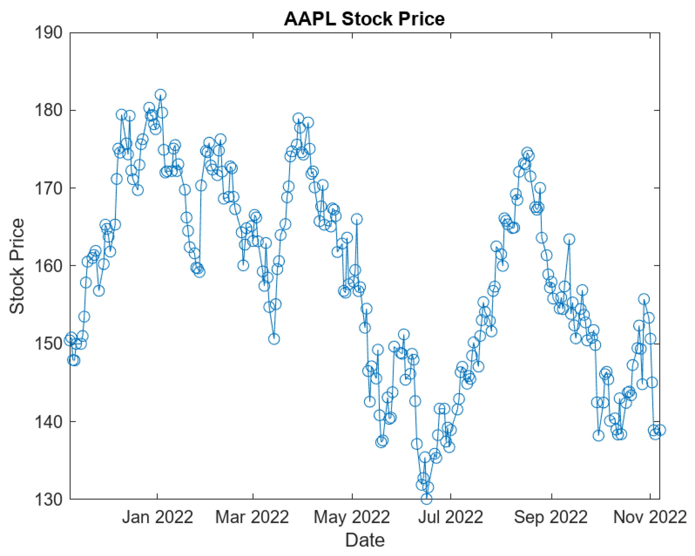
- AAPL Daily Closing Data at time :
Below, in Figure 3, a visualization of the daily closing price data of AAPL in the time period from November 2021 to November 2022.
- GOOG Daily Closing Data at time :
In Figure 4, below, we present a visualization depicting the daily closing price data of GOOG in the 1-year time period from November 2021 to November 2022.
5. Logarithmic Return of Stock Price
In order to calculate the realized pseudo-statistics and the expected pseudo-statistics for a future time period for the underlying stocks AAPL and GOOG, we must first calculate the logarithmic return of each stock price. Therefore, we need to define the logarithmic return and the arithmetic mean of the logarithmic returns. We will use the terminology and definitions found in (Badescu et al. 2002) Section 1.2, and the following equations, which can be found in (Badescu et al. 2002; Brockhaus and Long 2000; Carr and Lee 2009):
where .
where n is the number of logarithmic return data entries we need to calculate for each stock, and this number is 1 less than the total number of price data points. Using this information, along with Equations (15) and (16), we can now calculate the logarithmic returns and arithmetic mean of the logarithmic returns for the four data sets introduced in Section 4.
5.1. 6-Month Data Sets: Logarithmic Return and Arithmetic Mean
Using the data we described in Section 4.1, we can calculate the logarithmic return and the respective arithmetic means of the logarithmic returns of AAPL and GOOG over the 6-month period of November 2022 to May 2023, as follows:
- Logarithmic Return of AAPL:
Below, in Figure 5, we present an illustration depicting the daily logarithmic returns of AAPL that are calculated when Equation (15) is applied to the 6-month data set for AAPL described in Section 4.1.
- Arithmetic Mean of :
- Logarithmic Return of GOOG:
Below, in Figure 6, we present the values of the daily logarithmic returns of GOOG calculated using Equation (15) and the 6-month data set for GOOG described in Section 4.1.
- Arithmetic Mean of :
5.2. One-Year Data Sets: Logarithmic Return and Arithmetic Mean
In a similar fashion, we will now use the data we described in Section 4.2 to calculate the logarithmic return and the respective arithmetic means of the logarithmic returns of AAPL and GOOG over the 1-year period of November 2021 to November 2022, as follows:
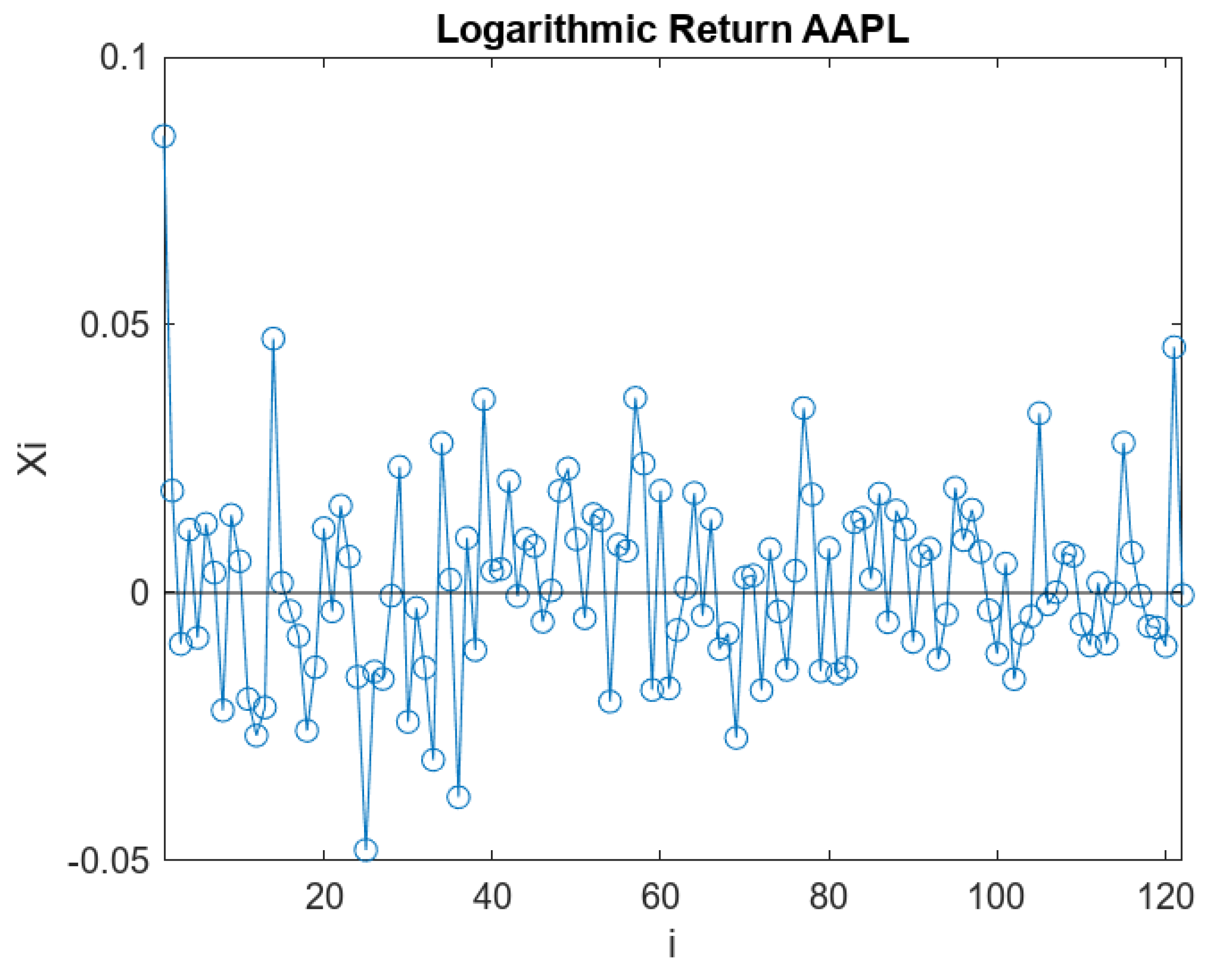
- Logarithmic Return of AAPL:
Below, we present Figure 7, which depicts the daily logarithmic returns of AAPL over the 1-year time period from November 2021 to November 2022, which were calculated using the 1-year data set for AAPL and Equation (15).
- Arithmetic Mean of :
- Logarithmic Return of GOOG:
In Figure 8, below, we present the daily logarithmic returns of GOOG over the 1-year time period from November 2021 to November 2022, which were calculated using the 1-year data set for GOOG and Equation (15).
- Arithmetic Mean of :
6. Expected Sample Variance and Brockhaus–Long Approximation for Expected Sample Volatility
In order to calculate the payoffs of pseudo-variance and volatility swaps, we must first calculate the expected sample variance and the expected sample volatility at the start of the swap contract, on 9 November 2022. In order to calculate the expected sample variance and volatility, we will use the Brockhaus–Long approximation (Brockhaus and Long 2000), and run a GARCH(1,1) regression on the logarithmic return data generated from the 1-year data sets introduced in Section 4.2, as was conducted in (Javaheri et al. 2004), while defining the following parameters:
- –
- Maturity Date in Years: T
- –
- Number of Logarithmic Return Entries: n.
- –
- GARCH(1,1) Constant: C
- –
- Kurtosis of Logarithmic Returns: .
Using the regression model and the parameters, we can then define the following formulas, which are dependent on the Heston model of securities markets, as described and derived in (Swishchuk 2004). We are using these formulas and the Heston model of securities markets, on which the formulas are based for comparison purposes, in order to obtain numerical values for the expected sample variance and volatility of a data set:
Having defined the previous equations and the parameters that go with them, we can now apply these equations to the AAPL and GOOG data sets.
6.1. AAPL: Expected Variance and Volatility
We will use the 1-year data set of AAPL daily closing price data that we introduced in Section 4.2, while assuming a maturity date of 6 months, from 9 November 2022. As a result, we have the following parameters:
- –
- Maturity Date in Years:
- –
- Number of Logarithmic Return Entries:
- –
- Kurtosis of AAPL Logarithmic Returns:
- –
- Short Volatility: .
We then apply a GARCH(1,1) regression on the logarithmic AAPL stock return data, the results of which are presented in Table 1, as follows:
From the data presented in Table 1, along with the parameters defined above and Equations (17)–(28), we can calculate the following results:
- Expected Sample Variance:
- Expected Sample Volatility:
6.2. GOOG: Expected Variance and Volatility
Similarly, we will use the 1-year data set of GOOG daily closing price data that we introduced in Section 4.2, while assuming a maturity date of 6 months, from 9 November 2022. As a result, we have the following parameters:
- –
- Maturity Date in Years:
- –
- Number of Logarithmic Return Entries:
- –
- Kurtosis of GOOG Logarithmic Returns:
- –
- Short Volatility: .
We then apply a GARCH(1,1) regression on the logarithmic GOOG stock return data, which results in Table 2, as follows:
From the data presented in Table 2, along with the parameters defined above and Equations (17)–(28), we can calculate the following results:
- Expected Sample Variance:
- Expected Sample Volatility:
7. Realized Pseudo-Volatility Square and Pseudo-Variance Swap Payoff
In order to calculate the realized pseudo-volatility square and the payoff of a pseudo-variance swap, we must first define the following parameters:
- –
- Position Taken:
- –
- Converting Parameter:
- –
- Strike Price: .
Using these parameters, we can then utilize the following pair of equations found in (Badescu et al. 2002), in order to calculate the realized pseudo-volatility square and pseudo-variance swap payoff:
Realized Pseudo-Volatility Square:
Payoff of Pseudo-Variance Swap:
We will use Equations (29) and (30), along with the defined parameters above, in the following sections, in order to calculate realized pseudo-volatility squares and pseudo-variance swap payoffs using the 6-month data sets introduced in Section 4.1.
7.1. AAPL: Realized Pseudo-Volatility Square and Pseudo-Variance Swap Payoff
Using the daily closing prices for AAPL in the 6-month period from November 2022 to May 2023, along with Equations (15), (16) and (29), we can calculate the realized pseudo-volatility square of AAPL to be the following:
- Realized Pseudo-Volatility Square of AAPL:
As previously calculated in Section 5.1, the mean of is 0.0021, which is the value we used to calculate the realized pseudo-volatility square above. However, we can examine the relationship between the realized pseudo-volatility square of AAPL and the arithmetic mean of the logarithmic AAPL stock returns by letting vary around its true value. As a result, we can produce Figure 9, which is below.
Now, using the realized pseudo-volatility square from November 2022 to May 2023 of the AAPL stock, which we calculated above, we can calculate the payoff of a pseudo-variance swap, whose underlying asset is the variance of the AAPL stock. We will assume the pseudo-variance swap has a maturity of 6 months, and that we are interested in the payoff associated with taking a long position on the swap. Additionally, we will assume that the payoff is calculated using a converting parameter of $1 per unit of pseudo-statistic, and we will use the expected sample variance of AAPL calculated in Section 6.1 as the strike price. Therefore, we now have the following parameter values:
- –
- Maturity Date:
- –
- Position Taken: .
- –
- Converting Parameter:
- –
- Strike Price: .
Using these parameters, Equation (16), and the previously calculated realized pseudo-volatility square of AAPL, we can calculate the payoff of a pseudo-variance, swap whose underlying asset is the variance of the AAPL stock, to be the following:
- Payoff of Pseudo-Variance Swap with Underlying of Variance of AAPL:
7.2. GOOG: Realized Pseudo-Volatility Square and Pseudo-Variance Swap Payoff
Similarly, we use the 6 months of daily closing prices for GOOG, along with Equations (15), (16) and (29), to calculate the realized pseudo-volatility square of GOOG to be the following:
- Realized Pseudo-Volatility Square of GOOG:
In Section 5.1, we found that is 0.0018; however, we can allow this value to vary in order to examine the relationship between the realized pseudo-volatility square of GOOG and the arithmetic mean of the logarithmic GOOG stock returns. As a result, we can produce Figure 10, which is included below.
Once again, we will calculate the payoff of a long position on a 6-month pseudo-variance swap with a conversion factor of 1. However, the underlying asset of the variance swap will now be the variance of GOOG, and we will use the expected sample variance of GOOG calculated in Section 6.2 as the strike price. Therefore, we will now use the following parameter values:
- –
- Maturity Date:
- –
- Position Taken:
- –
- Converting Parameter:
- –
- Strike Price: .
Using these parameters, Equation (30) and the previously calculated realized pseudo-volatility square of GOOG, we can calculate the payoff of a pseudo-variance swap whose underlying asset is the variance of the GOOG stock to be
- Payoff of Pseudo-Variance Swap with Underlying of Variance of GOOG:
8. Realized Pseudo-Volatility and Pseudo-Volatility Swap Payoff
To calculate the realized pseudo-volatility and the payoff of a pseudo-volatility swap, we must first define the following parameters:
- –
- Position Taken:
- –
- Converting Parameter:
- –
- Strike Price: .
Using these parameters allows us to utilize the following two equations, found in (Badescu et al. 2002), to calculate the realized pseudo-volatility and pseudo-volatility swap payoff:
Realized Pseudo-Volatility:
Payoff of Pseudo-Volatility Swap:
We will use Equations (31) and (32), along with the defined parameters above, in the following two sections, to calculate realized pseudo-volatilities and pseudo-volatility swap payoffs using the data sets first introduced in Section 4.1.
8.1. AAPL: Realized Pseudo-Volatility and Pseudo-Volatility Swap Payoff
Using Equations (15), (16) and (31), along with the daily closing prices for AAPL in the 6-month period from November 2022 to May 2023, we can calculate the realized pseudo-volatility of AAPL to be the following:
- Realized Pseudo-Volatility of AAPL:
Previously, in Section 5.1, we found that is equal to 0.0021, which we used above to calculate the realized pseudo-volatility. However, we can examine the relationship between the realized pseudo-volatility of AAPL and the arithmetic mean of the logarithmic AAPL stock returns by letting vary around its true value. As a result, we can produce Figure 11 below.
Using the realized pseudo-volatility calculated above, we can calculate the payoff of a pseudo-volatility swap, whose underlying asset is the volatility of the AAPL stock over the 6-month period from November 2022 to May 2023. We will assume the pseudo-variance swap has a maturity of 6 months, and that we are interested in the payoff associated with taking a long position on the swap. Additionally, we will assume that the payoff is calculated using a converting parameter of $1 per unit of pseudo-statistic, and we will use the expected sample volatility of AAPL calculated in Section 6.1 as the strike price. Therefore, we can now write the following parameter values:
- –
- Maturity Date:
- –
- Position Taken:
- –
- Converting Parameter:
- –
- Strike Price: .
Using these parameters along with Equation (32) and the previously calculated realized pseudo-volatility of AAPL, we can calculate the payoff of a pseudo-volatility swap, whose underlying asset is the volatility of the AAPL stock, to be the following:
- Payoff of Pseudo-Volatility Swap with Underling of Volatility of AAPL:
8.2. GOOG: Realized Pseudo-Volatility and Pseudo-Volatility Swap Payoff
Similarly, we can use the 6 months of daily closing prices for GOOG, along with Equation (15), (16) and (31), to calculate the realized pseudo-volatility of GOOG to be the following:
- Realized Pseudo-Volatility of GOOG:
In Section 5.1, we found that the mean of is equal to 0.0018, yet we can allow this value to vary in order to examine the relationship between the realized pseudo-volatility of GOOG and the arithmetic mean of the logarithmic GOOG stock returns. As a result, we can produce Figure 12 below.
Once again, we will calculate the payoff of a long position on a 6-month pseudo-volatility swap with a conversion factor of 1. However, the underlying asset of the volatility swap will now be the volatility of GOOG, and we will use the expected sample volatility of GOOG calculated in Section 6.2 as the strike price. Therefore, we will now use the following parameter values:
- –
- Maturity Date:
- –
- Position Taken:
- –
- Converting Parameter:
- –
- Strike Price: .
Using these parameters, Equation (32), and the previously calculated pseudo-volatility of GOOG, we can calculate the payoff of a pseudo-volatility swap, whose underlying asset is the volatility of the GOOG stock, to be:
- Payoff of Pseudo-Volatility Swap with Underling of Volatility of GOOG:
9. Expected Sample Covariance
In order to calculate the payoffs of pseudo-covariance swaps, we must first calculate the expected sample covariance at the start of the swap contract, on 9 November 2022. We will also use the equations and parameters we defined in Section 6, and we will again run a GARCH(1,1) regression on the logarithmic return data generated from the 1-year data sets introduced in Section 4.2. As a result, we can define the equation, found in (Swishchuk 2004), as follows:
Expected Sample Covariance:
where is calculated using Equation (25) defined in Section 6. Using these equations, we can now apply them to the AAPL () and GOOG (), 1-year data sets defined in Section 4.2, in order to calculate the expected sample covariance.
9.1. : Expected Variance
Using the 1-year data sets of daily closing prices of AAPL () and GOOG (), and multiplying each entry within them, we can form a new data set, denoted . This new data set, along with Equation (7) from Section 6, allows us to define the following parameters:
- –
- Maturity Date in Years:
- –
- Number of Logarithmic Return Entries:
- –
- Kurtosis of GOOG Logarithmic Returns:
- –
- Short Volatility: .
We then apply a GARCH(1,1) regression on the logarithmic return data, which results in Table 3, as follows:
From the data presented in Table 3, along with the parameters defined above and Equations (15)–(28), we can calculate the following results:
- Expected Sample Variance:
9.2. : Expected Variance
Similarly, we will use the 1-year data sets of daily closing prices of AAPL () and GOOG (), and divide each entry within them, to form a new data set, denoted , which, along with Equation (7) from Section 6, allows us to define the following parameters:
- –
- Maturity Date in Years:
- –
- Number of Logarithmic Return Entries:
- –
- Kurtosis of GOOG Logarithmic Returns:
- –
- Short Volatility: .
We then apply a GARCH(1,1) regression on the logarithmic return data, which results in Table 4, as follows:
From the data presented in Table 4, along with the parameters defined above and Equations (15)–(28), we can calculate the following results:
- Expected Sample Variance:
9.3. Calculating the Expected Sample Covariance of AAPL and GOOG
Using the results calculated above in Section 9.1 and Section 9.2, along with Equation (33), we can now calculate the expected covariance to be the following:
- Expected Sample Covariance of AAPL and GOOG:
10. Realized Pseudo-Volatility Cross and Pseudo-Covariance Swap Payoff
In order to calculate the realized pseudo-volatility cross and the payoff of a pseudo-covariance swap, we must first define the following parameters:
- –
- Position Taken:
- –
- Converting Parameter:
- –
- Strike Price: .
Using these parameters allows us to utilize the following pair of equations, found in (Badescu et al. 2002), to calculate the realized pseudo-volatility cross and pseudo-covariance swap payoff:
Realized Pseudo-Volatility Cross:
Payoff of Pseudo-Covariance Swap:
Using Equations (15), (16) and (34), along with the daily closing prices for AAPL and GOOG in the 6-month period from November 2022 to May 2023, we can calculate the realized pseudo-volatility cross of AAPL and GOOG to be the following:
- Realized Pseudo-Volatility Cross of AAPL and GOOG:
As previously calculated in Section 5.1, ; thus, we can allow to vary around its true value in order to allow us to examine the relationship between the realized pseudo-volatility cross of AAPL and GOOG over 6 months, and the arithmetic mean of the logarithmic AAPL stock returns. As a result, we can produce Figure 13, which is presented below.
Similarly, we can allow to vary around its true value of 0.0018 to examine the relationship between the realized pseudo-volatility cross of AAPL and GOOG over 6 months, and the arithmetic mean of the logarithmic GOOG stock returns. As a result, we can produce Figure 14, which is presented below.
Using the realized pseudo-volatility cross calculated above, we can calculate the payoff of a pseudo-covariance swap, whose underlying asset is the covariance of AAPL and GOOG stocks over the 6-month period from November 2022 to May 2023. We will assume the pseudo-covariance swap has a maturity of 6 months, and that we are interested in the payoff associated with taking a long position on the swap. Additionally, we will assume that the payoff is calculated using a converting parameter of $1 per unit of pseudo-statistic, and we will use the expected sample covariance calculated in Section 9.3 as the strike price. Therefore, we can now write the following parameter values:
- –
- Maturity Date:
- –
- Position Taken:
- –
- Converting Parameter:
- –
- Strike Price: .
Using these parameters, Equation (21), and the previously calculated pseudo-volatility cross of AAPL and GOOG, we can calculate the payoff of a pseudo-covariance swap, whose underlying asset is the covariance of AAPL and GOOG, to be
- Payoff of Pseudo-Covariance Swap with Underlying of Covariance of AAPL and GOOG:
11. Realized Pseudo-Correlation and Pseudo-Correlation Swap Payoff
In order to calculate the realized pseudo-correlation and the payoff of a pseudo-correlation swap, we must first define the following parameters:
- –
- Position Taken:
- –
- Converting Parameter:
- –
- Strike Price: .
Using these parameters allows us to utilize the following two equations, found in (Badescu et al. 2002), to calculate the realized pseudo-correlation and pseudo-correlation swap payoff:
Realized Pseudo-Correlation:
Payoff of Pseudo-Correlation Swap:
Using Equations (15), (16) and (36), along with the data sets of daily closing prices for AAPL and GOOG introduced in Section 4.1, we can calculate the realized pseudo-correlation of AAPL and GOOG to be the following:
- Realized Pseudo-Correlation of AAPL and GOOG:
Back in Section 5.1, we found that ; thus, in order to examine the relationship between the realized pseudo-correlation of AAPL and GOOG over 6 months, and the arithmetic mean of the logarithmic AAPL stock returns, we can allow to vary around its true value. As a result, we can produce Figure 15 below.
Similarly, we can allow to vary around its true value of 0.0018 to examine the relationship between the realized pseudo-correlation of AAPL and GOOG over 6 months, and the arithmetic mean of the logarithmic GOOG stock returns. In this case, we can produce Figure 16 below.
Using the realized pseudo-correlation calculated above, we can calculate the payoff of a pseudo-correlation swap, whose underlying asset is the correlation of AAPL and GOOG stocks over the 6-month period from November 2022 to May 2023. We will assume the pseudo-covariance swap has a maturity of 6 months, and that we are interested in the payoff associated with taking a long position on the swap. Additionally, we will assume that the payoff is calculated using a converting parameter of $1 per unit of pseudo-statistic. For the strike price we will use the realized pseudo-correlation achieved over the last 15 market days before the start of the swap contract on 9 November. Therefore, we can now write the following parameter values:
- –
- Maturity Date:
- –
- Position Taken:
- –
- Converting Parameter:
- –
- Strike Price: .
Using these parameters, Equation (37), and the previously calculated pseudo-correlation of AAPL and GOOG, we can calculate the payoff the payoff of a pseudo-correlation swap, whose underlying asset is the covariance of AAPL and GOOG, to be
- Payoff of Pseudo-Correlation Swap with Underlying of Covariance of AAPL and GOOG:
12. Comparing the Approach Based on the Cox–Ingresoll–Ross Model to the Realized Pseudo-Statistic Approach
The purpose of this section is to compare the payoffs of volatility and variance swaps, when the realized volatility and variance is calculated using the Cox–Ingresoll–Ross (CIR) model for variance rather than using the realized pseudo-statistic approach. The pseudo-statistic approach to calculating realized volatility and variance is a data/statistic approach that does not rely on a stochastic model for a stochastic stock price or stochastic volatility. Meanwhile, the Cox–Ingresoll–Ross (CIR) model is a stochastic volatility model that follows a stochastic differential equation (see (Swishchuk 2004)). Moreover, the Cox–Ingresoll–Ross (CIR) model is the most popularly used stochastic model for the calculation of variance, making it ideal for the comparison between a stochastic approach and a data/statistics approach to the pricing of swaps. Therefore, we will use the CIR model to create a comparison between a stochastic approach to pseudo-statistics and a data/statistical approach to pseudo-statistics in the following sections.
In the following two sections, we will calculate the realized variance and volatility of two stocks over a 6-month period, along with the payoffs of variance and volatility swaps, using the CIR model. Then, we will compare these calculated values to the payoffs of variance and volatility swaps associated with the same stocks over the same time period, which were calculated using the realized pseudo-statistic approach (see (Badescu et al. 2002)).
For the following report, we have used real-life financial data from Yahoo Finance (https://ca.finance.yahoo.com/ (accessed on 7 June 2023)) of the publicly traded stocks belonging to
- –
- Apple Inc. (AAPL)
- –
- Alphabet Inc. Class C (GOOG)
In the sections that follow, we will make use use of four data sets. The first two data sets contain 6 months of daily closing data for AAPL () and GOOG () from 9 November 2022 to 8 May 2023. The last two data sets contain 1 year of daily closing data for AAPL and GOOG from 8 November 2021 to 8 November 2022.
13. Realized Variance and Variance Swap Payoff
In order to calculate the realized variance using the Cox–Ingresoll–Ross (CIR) model, we will use the analytical closed form for discretely sampled variance, which is found in (Swishchuk 2004). The equation for the discretely sampled variance is as follows:
where T is the maturity date of the swap, n is one number less than the number of entries in the daily closing price data set, and is the daily closing price at time i.
Using Equation (38), we can calculate the realized sample variance according to the CIR model for AAPL and GOOG in the 6-month time period from November 2022 to May 2023, while making note of the remark that follows.
Remark 1.
Using the same two 6-month data sets, one can find that the realized pseudo-volatility square of AAPL is and the realized pseudo-volatility square of GOOG is .
13.1. Calculating the Realized Discretely Sampled Variance Using the CIR Model
Using the 6-month daily closing price data set for AAPL described in Section 12, while using the following parameters:
- –
- Maturity Date:
- –
- Number of Logarithmic Return Data Points: .
It is possible to use Equation (38) to calculate the AAPL realized discretely sampled variance from November 2022 to May 2023 to be the following:
- AAPL Realized Discretely Sampled Variance:
Comparing this value to the realized variance of AAPL obtained through the realized pseudo-statistic approach (see (Badescu et al. 2002)), one can observe that the value calculated above represents a increase over the realized variance of that is obtained with the realized pseudo-statistic approach.
Similarly, in order to calculate the realized variance over the 6 month period from November 2022 to May 2023 for GOOG, we will assume that
- –
- Maturity Date:
- –
- Number of Logarithmic Return Data Points: .
Then, we are able to use Equation (38) along with the 6-month daily closing price data set for GOOG described in Section 12, to calculate the GOOG realized discretely sampled variance to be
- GOOG Realized Discretely Sampled Variance:
Comparing this value to the realized variance of GOOG obtained through the realized pseudo-statistic approach (see (Badescu et al. 2002)), one can see that the value calculated above represents a increase over the realized variance of that is obtained with the realized pseudo-statistic approach.
13.2. Variance Swap Payoffs
In order to calculate the payoff of a variance swap, we must first define the following equation, which is found in (Swishchuk 2004):
where is the strike price, is the realized variance calculated using Equation (38), and N is the notional amount, as previously defined in Section 3.1.
The strike price values for both GOOG and AAPL will be the expected 6-month variance calculated using a GARCH(1,1) regression on the 1-year data sets described in Section 12. This approach is explained in detail in (Javaheri et al. 2004) and (Swishchuk 2004). The strike prices have been calculated to be
- –
- Strike Price AAPL
- –
- Strike Price GOOG .
Then, using Equation (39), the strike prices above, and a notional amount of , along with the previously calculated realized variance for AAPL and GOOG from Section 13.1, we can calculate the payoffs of the volatility swaps using the CIR model to be
- AAPL Variance Swap Payoff:
- GOOG Variance Swap Payoff:
These values are different from the variance swap payoffs calculated using the pseudo-statistic approach for realized variance (see (Badescu et al. 2002)). This is true, as if the pseudo-statistic approach is used, then the payoff of a swap whose underlying asset is the variance of AAPL is calculated to be , and if the underlying asset of the swap is the variance of GOOG, the swap payoff becomes .
14. Realized Volatility and Volatility Swap Payoff
In order to calculate the realized volatility using the Cox–Ingresoll–Ross (CIR) model, we will use the analytical closed form for discretely sampled volatility. The equation for discretely sampled volatility is found in (Swishchuk 2004), and it can be defined as follows:
where is the realized discretely sampled variance that was defined by Equation (38).
Using Equation (40), we can calculate the realized volatility according to the CIR model for AAPL and GOOG in the 6-month time period from November 2022 to May 2023, while making note of the remark that follows.
Remark 2.
The realized pseudo-volatility of AAPL over the same 6-month time period is , while the realized pseudo-volatility of GOOG from November 2022 to May 2023 is .
14.1. Calculating the Realized Discretely Sampled Volatility Using the CIR Model
Using the 6-month daily closing price data set for AAPL described in Section 12, we previously calculated in Section 13.1 that the realized discretely sampled variance for AAPL from November 2022 to May 2023 is . Therefore, we can use Equation (40) to calculate the realized discretely sampled volatility over the 6-month time period for AAPL to be:
- AAPL Realized Discretely Sampled Volatility:
Comparing this value to the realized volatility of AAPL obtained through the realized pseudo-statistic approach (see (Badescu et al. 2002)), one can see that the value calculated above represents a increase over the realized volatility of that is calculated if using the realized pseudo-statistic approach.
Similarly, in Section 13.1, we found that the realized discretely sampled variance of GOOG over the 6-month period from November 2022 to May 2023 is . Therefore, using Equation (40), we can calculate the realized discretely sampled volatility over the 6-month time period of November 2022 to May 2023 to be:
- GOOG Realized Discretely Sampled Volatility:
Comparing this value to the realized volatility of GOOG obtained through the realized pseudo-statistic approach (see (Badescu et al. 2002)), one can see that the value calculated above represents a increase over the realized volatility of that is calculated if using the realized pseudo-statistic approach.
14.2. Volatility Swap Payoffs
In order to calculate the payoff of a volatility swap, we must first define the equation, found in (Swishchuk 2004), as follows:
where is the strike price, is the realized volatility calculated using Equation (40), and N is the notional amount, as previously defined in Section 3.1.
The strike price values for both GOOG and AAPL will be the expected 6-month volatility calculated using a GARCH(1,1) regression (see (Swishchuk 2004) and (Javaheri et al. 2004)) and the Brockhaus–Long approximation (see (Brockhaus and Long 2000)) on the 1-year data sets described in Section 12. The strike prices have been calculated to be
- –
- Strike Price AAPL
- –
- Strike Price GOOG .
Using these strike prices, a notional amount of , Equation (41), and the previously calculated realized volatility for AAPL and GOOG from Section 14.1, we can calculate the payoffs of the volatility swaps, using the CIR model, to be:
- AAPL Volatility Swap Payoff:
- GOOG Volatility Swap Payoff:
These values differ from the volatility swap payoffs calculated using the pseudo-statistic approach for realized volatility (see (Badescu et al. 2002)). If the pseudo-statistic approach is used, then the payoff for a swap whose underlying asset is the volatility of AAPL is calculated to be , and if the underlying asset of the swap is the volatility of GOOG, then the swap payoff becomes .
15. Conclusions and Future Work
In accordance with the main motivation of this paper, which was described in Section 1, in the previous sections of this paper, we have considered the pricing of swaps based on pseudo-statistics, instead of stochastic models, and we have compared this approach with the most popular stochastic volatility model in the Cox–Ingresoll–Ross (CIR) model. Within this paper, we have demonstrated how to price various types of swaps (variance, volatility, covariance, and correlation swaps) using pseudo-statistics (pseudo-variance, pseudo-volatility, pseudo-correlation, and pseudo-covariance). We have also presented analytical closed-form formulas for both the pseudo-statistics and the pricing of swaps based on these pseudo-statistics. As a result, within this paper, we present a method for pricing swaps that does not rely on any stochastic models for a stochastic stock price or stochastic volatility, and instead relies on data/statistics. Consequently, using real-life data along with this data/statistical approach to swap pricing, we were able to calculate numerical values for the value of various swaps based on the volatility, variance, covariance, and correlation of AAPL and GOOG. Some of these results are summarized below in Table 5.
The data/statistics-based approach to swap pricing we have introduced is very different from stochastic volatility models such as the Cox–Ingresoll–Ross (CIR) model, which, in comparison, follows a stochastic differential equation (see (Swishchuk 2004)). Therefore, in this paper, we have compared the CIR model approach to pricing swaps to the pseudo-statistic approach to pricing swaps, in order to compare a stochastic model to the data/statistics-based approach to swap pricing, which was developed within this paper. Although there are many other stochastic models that provide an approach to calculating the price of swaps, we have used the CIR model for comparison within this paper, due to the popularity of the CIR model.
After using Section 12 to define the four data sets that were to be used in the calculations of Section 13 and Section 14, along with providing a short description of the approach that was to be used, we were able to use the Cox–Ingresoll–Ross (CIR) model to calculate the realized discretely sampled variance of AAPL and GOOG over a 6-month period of November 2022 to May 2023 in Section 13.1, the variance swap payoffs in Section 13.2, the realized discretely sampled volatility in Section 14.1, and the volatility swap payoffs in Section 14.2.
Consequently, we were able to compare these values to previously calculated values, which were obtained using the same time period and the same data sets, but with the realized pseudo-statistic approach (see (Badescu et al. 2002)). Although the values obtained through the realized pseudo-statistic approach were similar to the values obtained through the CIR model, differences between the values did exist, as can be seen in Table 5 below:
As a result, through the calculations contained within this report, we can conclude that realized volatility and variance, as well as the payoffs associated with volatility and variance swaps, can be calculated with either the CIR model or the realized pseudo-statistic approach, and similar results will be obtained. However, it is clear that even though the results will be similar depending on the approach used, the resulting values will not be identical.
In future work, we plan to further research the comparison between the data/statistical approach to swap pricing and the stochastic approach to swap pricing, beyond the Cox–Ingresoll–Ross (CIR) model. Therefore, future work could include comparing the pseudo-statistic approach to the non-Gaussian Ornstein–Uhlenbeck stochastic volatility model, using the information in (Benth et al. 2007) as a framework for calculating volatility under the Ornstein–Uhlenbeck model. Other stochastic models that should be compared to the data/statistical approach to calculating volatility include the BN-S stochastic volatility model (see (Sengupta 2016)), delayed volatility swaps (see (Swishchuk and Vadori 2014)), and Markov-modulated volatilities (see (Salvi and Swishchuk 2014)).
Author Contributions
Conceptualization, A.S.; methodology, A.S.; software, S.F.; validation, A.S.; formal analysis, S.F.; investigation, S.F.; data curation, S.F.; writing—original draft preparation, S.F.; writing—review and editing, A.S.; visualization, S.F.; supervision, A.S.; project administration, A.S. All authors have read and agreed to the published version of the manuscript.
Funding
This research received no external funding.
Data Availability Statement
The real-life financial data that were used within the calculations of this article can be found at (http://ca.finance.yahoo.com/ (accessed on 7 June 2023)). The 6-month data set for AAPL can be found at (https://ca.finance.yahoo.com/quote/AAPL/history?period1=1667952000&period2=1683590400&interval=1d&filter=history&frequency=1d&includeAdjustedClose=true (accessed on 7 June 2023)). The 6-month data set for GOOG can be found at (https://ca.finance.yahoo.com/quote/GOOG/history?period1=1667952000&period2=1683590400&interval=1d&filter=history&frequency=1d&includeAdjustedClose=true (accessed on 7 June 2023)). The 1-year data set for AAPL can be found at (https://ca.finance.yahoo.com/quote/AAPL/history?period1=1636329600&period2=1667865600&interval=1d&filter=history&frequency=1d&includeAdjustedClose=true (accessed on 7 June 2023)). The 1-year data set for GOOG can be found at (https://ca.finance.yahoo.com/quote/GOOG/history?period1=1636329600&period2=1667865600&interval=1d&filter=history&frequency=1d&includeAdjustedClose=true (accessed on 7 June 2023)).
Acknowledgments
The authors thank NSERC for continuing support.
Conflicts of Interest
The authors declare no conflict of interest.
Abbreviations
The following abbreviations are used in this manuscript:
| MDPI | Multidisciplinary Digital Publishing Institute |
| CIR | Cox–Ingresoll–Ross |
| AAPL | Apple Inc. |
| GOOG | Alphabet Inc. Class C |
References
- Badescu, Andrei, Anatoliy Swishchuk, Raymond Cheng, Stephan Lawi, Hammouda Mekki, Asrat Gashaw, Yuanyuan Hua, Marat Molyboga, Tereza Neocleous, and Yuri Petratchenko. 2002. Price Pseudo-Variance, Pseudo-Covariance, Pseudo-Volatility, and Pseudo-Correlation Swaps-In Analytical Closed-Forms. In Sixth PIMS Industrial Problems Solving Workshop. Vancouver: University of British Columbia, pp. 45–55. [Google Scholar]
- Benth, Fred Espen, Martin Groth, and Rodwell Kufakunesu. 2007. Valuing Volatility and Variance Swaps for a Non-Gaussian Ornstein–Uhlenbeck Stochastic Volatility Model. Applied Mathematical Finance 14: 347–63. [Google Scholar] [CrossRef]
- Brenner, Menachem, and Dan Galai. 1989. New Financial Instruments for Hedging Changes in Volatility. Financial Analysts Journal 45: 61–65. [Google Scholar] [CrossRef]
- Brenner, Menachem, and Dan Galai. 1993. Hedging Volatility in Foreign Currencies. The Journal of Derivatives 1: 53–59. [Google Scholar] [CrossRef]
- Brenner, Menachem, and Dan Galai. 1996. Options on Volatility. In Option Embedded Bonds: Price Analysis, Credit Risk and Investment Strategies. Edited by Israel Nelken. New York: Irwin Professional Pub, pp. 273–86. [Google Scholar]
- Brockhaus, Oliver, and Douglas Long. 2000. Volatility Swaps Made Simple. Risk-London Magazine Limited 13: 92–96. [Google Scholar]
- Carr, Peter, and Dilip Madan. 2001. Towards a theory of volatility trading. In Option Pricing, Interest Rates and Risk Management, Handbooks in Mathematical Finance. Cambridge: Cambridge University Press, vol. 22, pp. 458–76. [Google Scholar]
- Carr, Peter, and Roger Lee. 2009. Volatility Derivatives. Annual Review of Financial Economics 1: 319–39. [Google Scholar] [CrossRef] [Green Version]
- Demeterfi, Kresimir, Emanuel Derman, Michael Kamal, and Joseph Zou. 1999. A guide to volatility and variance swaps. The Journal of Derivatives 6: 9–32. [Google Scholar] [CrossRef]
- Derman, Emanuel, Iraj Kani, and Michael Kamal. 1997. Trading and hedging local volatility. Journal of Financial Engineering 6: 233–68. [Google Scholar]
- Dupire, Bruno. 1993. Model art. Risk 6: 118–24. [Google Scholar]
- Dupire, Bruno. 1996. A unified theory of volatility. In Derivatives Pricing: The Classic Collection. London: Risk Books London, pp. 185–96. [Google Scholar]
- Fleming, Jeff, Barbara Ostdiek, and Robert E. Whaley. 1995. Predicting stock market volatility: A new measure. The Journal of Futures Markets (1986–1998) 15: 265. [Google Scholar]
- Galai, Dan. 1979. A proposal for indexes for traded call options. The Journal of Finance 34: 1157–72. [Google Scholar] [CrossRef]
- Gastineau, Gary L. 1977. An index of listed option premiums. Financial Analysts Journal 33: 70–75. [Google Scholar] [CrossRef]
- Grünbichler, Andreas, and Francis A. Longstaff. 1996. Valuing futures and options on volatility. Journal of Banking & Finance 20: 985–1001. [Google Scholar]
- Habtemicael, Semere, and Indranil Sengupta. 2016a. Pricing Covariance Swaps for Barndorff-Nielsen and Shephard Process Driven Financial Markets. Annals of Financial Economics 11: 1650012. [Google Scholar] [CrossRef]
- Habtemicael, Semere, and Indranil Sengupta. 2016b. Pricing Variance and Volatility Swaps for Barndorff-Nielsen and Shephard Process Driven Financial Markets. International Journal of Financial Engineering 3: 1650027. [Google Scholar] [CrossRef]
- Issaka, Aziz, and Indranil SenGupta. 2017. Analysis of Variance based Instruments for Ornstein–Uhlenbeck Type Models: Swap and Price Index. Annals of Finance 13: 401–34. [Google Scholar] [CrossRef]
- Javaheri, Alireza, Paul Wilmott, and Espen Haug. 2004. GARCH and Volatility swaps. Quantitative Finance 4: 589–95. [Google Scholar] [CrossRef]
- Neuberger, Anthony. 1994. The Log Contract. The Journal of Portfolio Management 20: 74–80. [Google Scholar] [CrossRef]
- Neuberger, Anthony J. 1990. Volatility Trading. London: Institute of Finance and Accounting, London Business School. [Google Scholar]
- Salvi, Giovanni, and Anatoliy V. Swishchuk. 2014. Covariance and Correlation Swaps for Financial Markets with Markov-Modulated Volatilities. International Journal of Theoretical and Applied Finance 17: 1450006. [Google Scholar] [CrossRef]
- Schoutens, Wim. 2005. Moment swaps. Quantitative Finance 5: 525–30. [Google Scholar] [CrossRef]
- Sengupta, Indranil. 2016. Generalized BN-S Stochastic Volatility Model for Option Pricing. International Journal of Theoretical and Applied Finance 19: 1650014. [Google Scholar] [CrossRef]
- Swishchuk, Anatoliy. 2004. Modeling of Variance and Volatility Swaps for Financial Markets with Stochastic Volatilities. Wilmott Magazine 2: 64–72. [Google Scholar]
- Swishchuk, Anatoliy. 2005. Modelling and Pricing for Stochastic Volatilities with Delay. Wilmott Magazine 19: 63–73. [Google Scholar]
- Swishchuk, Anatoliy. 2006. Modeling and pricing of variance swaps for multi-factor stochastic volatilities with delay. Canadian Applied Mathematics Quarterly 14: 439–67. [Google Scholar]
- Swishchuk, Anatoliy, and Nelson Vadori. 2014. Smiling for the Delayed Volatility Swaps: Smiling for the Delayed Volatility Swaps. Wilmott 2014: 62–73. [Google Scholar] [CrossRef] [Green Version]
- RBC Financial Group Team. 2002. Price Pseudo-Variance, Pseudo-Covariance, Pseudo-Volatility, and Pseudo-Correlation Swaps-in Analytical Close Form. In Proceedings of the 6th Annual PIMS Industrial Problem Solving Workshop. Vancouver: University of British Columbia. [Google Scholar]
- Whaley, Robert E. 1993. Derivatives on market volatility: Hedging tools long overdue. The Journal of Derivatives 1: 71–84. [Google Scholar] [CrossRef]
Figure 1.
AAPL stock price over a 6-month period of November 2022 to May 2023.

Figure 2.
GOOG stock price over a 6-month period of November 2022 to May 2023.

Figure 3.
AAPL stock price over a 1-year period of November 2021 to November 2022.

Figure 4.
GOOG stock price over a 1-year period of November 2021 to November 2022.

Figure 5.
AAPL Logarithmic returns over a 6-month period of November 2022 to May 2023.

Figure 6.
GOOG Logarithmic returns over a 6-month period of November 2022 to May 2023.

Figure 7.
AAPL Logarithmic returns over a 1-year period of November 2021 to November 2022.

Figure 8.
GOOG Logarithmic returns over a 1-year period of November 2021 to November 2022.

Figure 9.
Realized pseudo−volatility square of AAPL from November 2022 to May 2023, as a function of .
Figure 9.
Realized pseudo−volatility square of AAPL from November 2022 to May 2023, as a function of .

Figure 10.
Realized pseudo−volatility square of GOOG from November 2022 to May 2023, as a function of .
Figure 10.
Realized pseudo−volatility square of GOOG from November 2022 to May 2023, as a function of .

Figure 11.
Realized pseudo−volatility of AAPL from November 2022 to May 2023, as a function of .

Figure 12.
Realized pseudo−volatility of GOOG from November 2022 to May 2023, as a function of .

Figure 13.
Realized pseudo−volatility cross of AAPL and GOOG from November 2022 to May 2023, as a function of .
Figure 13.
Realized pseudo−volatility cross of AAPL and GOOG from November 2022 to May 2023, as a function of .

Figure 14.
Realized pseudo−volatility cross of AAPL and GOOG from November 2022 to May 2023, as a function of .
Figure 14.
Realized pseudo−volatility cross of AAPL and GOOG from November 2022 to May 2023, as a function of .

Figure 15.
Realized pseudo−correlation of AAPL and GOOG from November 2022 to May 2023, as a function of .
Figure 15.
Realized pseudo−correlation of AAPL and GOOG from November 2022 to May 2023, as a function of .

Figure 16.
Realized pseudo−correlation of AAPL and GOOG from November 2022 to May 2023, as a function of .
Figure 16.
Realized pseudo−correlation of AAPL and GOOG from November 2022 to May 2023, as a function of .


Table 1.
GARCH(1,1) regression on AAPL logarithmic returns.
| Value | Standard Error | T Statistic | p Value | |
|---|---|---|---|---|
| Constant | ||||
| GARCH{1} | ||||
| ARCH{1} |
Table 2.
GARCH(1,1) regression on GOOG logarithmic returns.
| Value | Standard Error | T Statistic | p Value | |
|---|---|---|---|---|
| Constant | ||||
| GARCH{1} | ||||
| ARCH{1} |
Table 3.
GARCH(1,1) regression on logarithmic returns.
| Value | Standard Error | T Statistic | p Value | |
|---|---|---|---|---|
| Constant | ||||
| GARCH{1} | ||||
| ARCH{1} |
Table 4.
GARCH(1,1) regression on logarithmic returns.
| Value | Standard Error | T Statistic | p Value | |
|---|---|---|---|---|
| Constant | ||||
| GARCH{1} | 1 | |||
| ARCH{1} | 1 |
Table 5.
Summary of results presented in sections above.
| Value Obtained November 2022 to May 2023 | Using CIR Model | Using Realized Pseudo-Statistic Approach |
|---|---|---|
| AAPL Realized Variance | 0.0816 | 0.0805 |
| GOOG Realized Variance | 0.1277 | 0.1269 |
| AAPL Variance Swap Payoff | 0.0684 | 0.0673 |
| GOOG Variance Swap Payoff | 0.1094 | 0.1086 |
| AAPL Realized Volatility | 0.2856 | 0.2838 |
| GOOG Realized Volatility | 0.3574 | 0.3563 |
| AAPL Volatility Swap Payoff | 0.1758 | 0.1740 |
| GOOG Volatility Swap Payoff | 0.2307 | 0.2296 |
Disclaimer/Publisher’s Note: The statements, opinions and data contained in all publications are solely those of the individual author(s) and contributor(s) and not of MDPI and/or the editor(s). MDPI and/or the editor(s) disclaim responsibility for any injury to people or property resulting from any ideas, methods, instructions or products referred to in the content. |
© 2023 by the authors. Licensee MDPI, Basel, Switzerland. This article is an open access article distributed under the terms and conditions of the Creative Commons Attribution (CC BY) license (https://creativecommons.org/licenses/by/4.0/).
Share and Cite
MDPI and ACS Style
Franco, S.; Swishchuk, A. Pricing of Pseudo-Swaps Based on Pseudo-Statistics. Risks 2023, 11, 141. https://doi.org/10.3390/risks11080141
AMA Style
Franco S, Swishchuk A. Pricing of Pseudo-Swaps Based on Pseudo-Statistics. Risks. 2023; 11(8):141. https://doi.org/10.3390/risks11080141
Chicago/Turabian StyleFranco, Sebastian, and Anatoliy Swishchuk. 2023. "Pricing of Pseudo-Swaps Based on Pseudo-Statistics" Risks 11, no. 8: 141. https://doi.org/10.3390/risks11080141
Note that from the first issue of 2016, this journal uses article numbers instead of page numbers. See further details here.