1. Introduction
Pairs trading is a widely used strategy for traders and fund managers. It involves taking simultaneous positions in two correlated assets and speculating on the path behavior of the resulting spread. While it is difficult to fully model the dynamics of a single asset, a pair of assets or securities may exhibit mean reverting behavior that can be better captured by statistical models.
Each pairs trading strategy involves three main steps: (i) identification of assets, (ii) formation of spreads, and (iii) design of trading rules. While there are various ways to select assets for pairs trading, the two price processes for each pair should exhibit an adequate degree of comovement so that the resulting spread is mean reverting. In such a case, trading opportunities arise when the spread deviates from its mean.
We adopt a statistical approach to pairs trading. For any given pair of stocks, we construct the spread such that it best fits the Ornstein–Uhlenbeck (OU) model. Specifically, we determine the optimal ratio between two stocks, along with the model parameters, such that the resulting spread time series achieves the maximum likelihood. This method is an extension of the maximum likelihood estimation (MLE) approach which typically only determines the model parameters. With the spread formed, we apply a set of trading rules. The critical levels to enter and exit are set at a multiple of the standard deviation from the long-term mean of spread. For more details, we refer to
Lee and Leung (
2020) and references therein.
To our best knowledge, existing studies on pairs trading analyze the performance of a single pair, rather than the aggregate performance of multiple pairs. There are several practical benefits of trading multiple pairs and considering them together in a trading program. Firstly, more spreads may give rise to more trading opportunities at any point in time. Secondly, the spreads generated from different stocks are likely to be mostly uncorrelated, which makes it an ideal setting to take advantage of diversification. Lastly, trading multiple pairs also opens up a new direction for portfolio optimization, which does not exist when trading a single pair.
In this paper, we propose a novel framework for constructing diversified portfolios from multiple pairs trading strategies. Capital is allocated among different pairs based on the statistical characteristics, such as the speed of mean reversion and volatility, of the historical spreads. Moreover, our approach is adaptive as portfolio weights are adjusted periodically. Among our allocation methods, we introduce the novel Mean Reversion Budgeting (MRB) and Mean Reversion Ranking (MRR) methods. The MRB method determines the portfolio weights based on the speeds of mean reversion, volatilities, and estimated average log-likelihood scores together. In contrast, the MRR method ranks spreads based on their estimated likelihood scores and speeds of mean reversion and assigns prespecified portfolio weights based on the rankings of the spreads.
Working with the empirical price data of six stock pairs, our experiment suggests that the proposed framework offers some desirable return profiles and portfolio features. We compare several allocation methods to the benchmark equal-weight portfolio and illustrate how dynamic rebalancing can improve portfolio performance.
The rest of the paper is organized as follows. We provide a review of related studies in
Section 2. In
Section 3, we outline the steps of portfolio construction and trading rules for mean reversion trading. As part of
Section 4, we demonstrate how the volatility of spreads and speed of mean reversion affect the performance of simulated trades. In
Section 5, we describe the proposed diversification framework.
Section 6 describes the asset pairs included in our study, and our data collection process, and compares the performance of the proposed framework to the baseline. Concluding remarks are provided in
Section 7.
2. Related Studies
Gatev et al. (
2006) provided one of the first in-depth studies on pairs trading. They proposed a commonly used Distance Method (DM) and test the CRSP stocks from 1962 to 2002. The DM method opens a position for a pair when the prices diverge from 0 by more than two historical standard deviations and closes the position at the next crossing of the prices. They reported an excess return of 1.3% for the top 5 pairs of the DM, and 1.4% for its top 20 pairs.
Do and Faff (
2012) examined the profitability of pairs trading accounting for transaction costs.
Other than the DM method, the cointegration test is commonly used in many alternative methods for mean reversion trading.
Vidyamurthy (
2004) detailed a cointegration framework for mean reversion trading based on the Engle and Granger’s error correction model representation of cointegrated series presented in
Engle and Granger (
1987).
Galenko et al. (
2012) examined an active ETF trading strategy based on cointegrated time series.
Leung and Nguyen (
2019) constructed cointegrated portfolios of cryptocurrencies using the Engle–Granger two-step approach and Johansen cointegration test.
Huck and Afawubo (
2015) compared the performance of DM and cointegration method using the components of the S&P 500 index.
Another popular approach, the stochastic spread method, captures the path behavior of the spread through a stochastic process with mean-reverting property, such as the Ornstein–Uhlenbeck (OU) process. The construction of spreads and extraction of trading signals are typically derived from the analysis of parameters of the underlying model.
Elliott et al. (
2005) proposed a mean-reverting Gaussian Markov chain model to describe spread dynamics. The model’s estimates are compared with observations of the spread to determine appropriate trading decisions.
Do et al. (
2006) further analyzed the method proposed by
Elliott et al. (
2005) and proposed a general stochastic residual spread method to model relative mispricing.
Leung and Li (
2015) studied the optimal timing strategies for mean-reverting trading under the OU process. They solved an optimal double-stopping problem to analyze the timing of entry and liquidation subject to transaction costs.
Lee and Leung (
2020) examined the performance of mean reversion trading using dynamically optimized entry and exit rules.
Finally, we note that all the studies mentioned above focus on the trading performance of a single pair. The proposed framework herein is designed for trading multiple pairs simultaneously and is optimized as a diversified portfolio.
3. Pairs Construction and Trading Rules
We construct a long-short position with two highly correlated assets
and
. The portfolio value is given by
where the coefficient
B is called the hedge ratio and can be optimized. Following the procedure detailed in
Leung and Li (
2016, chp. 2), we determine the optimal pair ratio through maximum likelihood estimation (MLE), whereby the resulting historical spread time series best fits the Ornstein–Uhlenbeck (OU) model.
An OU process is a mean-reverting process, described by the following stochastic differential equation:
where
represents the speed of mean reversion,
is the long-term mean, and
is the volatility parameter. Here,
is a standard Brownian motion under the historical measure
.
3.1. Statistical Estimation for Optimized Mean Reversion
For any given hedge ratio
b, consider the observed time series of the resulting spread
up to time
. Then, we apply the method of maximum likelihood estimation to determine the optimal parameters for the OU model based on the historical data. Specifically, given
with time increment
, define the average log-likelihood function of the past
L observations as
where
To express the OU parameter values that maximize the average log-likelihood in (2), we define the following:
In turn, the optimal parameter estimates under the OU model are given explicitly by
At this stage, we maximize the average log-likelihood function over the three OU model parameters and denote the maximized average log-likelihood by
Then, the maximized log-likelihood function
is further optimized over the ratio
b to give the optimal hedge ratio
In practice, the implementation of this optimization can be done via a grid search. For instance, suppose we limit the absolute value of the hedge ratio to be 2. Then, we compute the maximized log-likelihood function
for
The maximizer is denoted by B.
3.2. Trading Rules
We now describe the mechanism of the trading strategy in this study. Denote by and the prices of two assets at time t. Let be the capital available at time t. The initial investment amount is .
A number of indicators are required in order to set up the trading signals. We consider the M-day moving average of the spread , denoted by . Similarly, we define to be the standard deviation of the spread over the past M-days. We use the notations and for positions of and . Finally, K is the trading threshold, r is the chosen risk level for the stop-loss rule, L is the length of the lookback window, and T is the length of the entire trading period.
In turn, the trading strategy is described as follows.
In Step 3, a long position of is established if no shares of are held and the price of drops below the past M-days average value minus K times standard deviation. The number of shares purchased is determined by the ratio of current cash and price of . That is, invest all the cash at hand to long and short the corresponding with the best pair ratio B.
As for the liquidation rule described in Step 4, the entire position is liquidated whenever the price of
rises beyond the past
M-days average value. In short, we enter the long position if the price of spread drops sufficiently far from the long-term mean, and then wait for the price to revert and take profit. The trading rule for short positions follows a similar logic. For more details on this approach, we refer to
Lee and Leung (
2020) and the references therein.
The trading system includes four parameters: L is the length of look-back window length that determines how many data points are used to estimate the best ratio; T determines how long we will use the estimated best ratio; M is the number of days used to calculate the moving average and standard deviation of the spread, and K is the threshold that determines the trading boundary.
Intuitively, L and M control how much past data should be incorporated in the current trading decisions. The other parameter, K, will have direct influence on the timing and frequency of trades. For instance, a smaller K will result in more frequent trading.
4. Monte Carlo Simulation
In this section, we analyze how different degrees of mean reversion may impact trading performance via Monte Carlo simulation. This analysis will shed light on capital allocation across different spreads in our diversification framework.
We begin by considering trading a single spread, whose values are simulated according to the OU model. There are three parameters in the model. The speed of mean reversion is denoted by , the volatility of the process is denoted by , and the long-term mean is . We generate 1000 sample paths with different combinations of parameters and simulate the trading transactions over one year () for each path by following the rule described in the previous section.
We examine the trading performance through the Sharpe ratio, average daily return, volatility, total trading numbers, and cumulative return, which are calculated based on the average over 1000 paths. The other parameters of the trading system are and in this experiment. Since we generate the spread time series directly, there is no need to compute the optimal pair ratio.
The results are summarized in
Table 1. Among the parameters, we observe that the speed of mean reversion
has a significant effect on the performance. Raising
with
and
constant, the daily returns, Sharpe ratio, and number of trades all increase while the standard deviation decreases slightly. This is intuitive since a fast mean-reverting spread offers more trading opportunities and reduces the risk associated with the trading strategy.
Next, we examine the effect of the spread volatility . For different with and , the Sharpe ratio is almost unchanged since both daily returns and volatility increase simultaneously as increases. Intuitively, higher volatility may offer more trading opportunities as the spread fluctuates more rapidly. However, higher volatility also leads to a wider trading band, thus increasing the risk exposure. Lastly, the long-term mean does not have a significant impact on trading performance as expected, given that trades are triggered by the deviation of the spread from the long-term mean.
Based on the simulation results, the speed of mean reversion has a significantly positive effect on performance as measured by average return and Sharpe ratio. Moreover, a faster spread of mean reversion also results in more frequent trades. On the other hand, the spread volatility increases the mean and standard deviation of returns simultaneously, so the Sharpe ratio is lower for very high volatility. In contrast, the long-term mean does not affect the trading performance materially. Hence, we consider the mean reversion rate as a critical factor when designing the diversification framework for trading multiple pairs.
5. Diversification Framework
We consider a diversified portfolio approach to trading multiple pairs simultaneously. This leads to the analysis of a number of different methods to allocate portfolio weights to the traded pairs.
The first step is to divide the entire trading period into stages with a defined schedule for adjusting the allocation. During the first trading stage, we apply equal weights to trade all the spreads in the portfolio. After that, empirical spreads and returns are recorded and analyzed to yield an optimal allocation for the next trading stage. Moving forward, we will periodically obtain updates on the portfolio weights and re-allocate the capital for the next trading period accordingly.
5.1. Portfolio Weights
In our framework, capital is allocated across different pairs in order to form a diversified portfolio. There are various methods to determine the portfolio weights dynamically over time. To that end, we consider several methods and examine their effects on portfolio performance.
5.1.1. Mean-Variance Analysis
Inspired by Mean-Variance Analysis (MVA), one method for determining the portfolio weights is by maximizing the Sharpe ratio. For any given lookback period, let
be the vector of average returns of each pair and
be the corresponding co-variance matrix of daily returns of each pair. Then, the optimal weights are those that give the best historical in-sample Sharpe ratio. Precisely, we have
This MVA-based method assumes that the weights that have produced the best Sharpe ratio in the recent past will lead to a good performance in the next trading period. This depends on the stability of the returns over time, which may not be a reliable assumption. To address this issue, we propose several alternative allocation methods based on the characteristics of the spreads, rather than returns.
5.1.2. Mean Reversion Budgeting
We propose an allocation method, called Mean Reversion Budgeting (MRB), which is based on the mean-reverting properties of the spreads. In essence, we seek to measure the degree of mean reversion for each spread and assign more weights to those that are considered highly mean-reverting.
The first index is the estimated maximum average log-likelihood function.
To measure the goodness of fit to an OU process for each spread, we consider the corresponding log-likelihood score. For each spread
i, we denote by
the estimated maximum average log-likelihood score from the previous stage. Next, we do min-max normalization to make them all positive. Precisely, for each spread
i, we define the index:
In addition, we consider the speed of mean reversion
. Intuitively, a more rapidly mean-reverting spread offers more trading opportunities, so it should be allocated with more portfolio weights. In order to account for the fluctuations due to volatility, we scale the speed of mean reversion by the volatility parameter. Precisely, we write
where
and
are, respectively, the estimated speed of mean reversion and volatility for each pair. In turn, comparing across all spreads, we define the normalized relative speed of mean reversion for spread
i as
Lastly, we incorporate both
and
into the portfolio weight allocation. This results in the formula
In summary, this means that more capital is allocated into pairs that are more OU-like and mean-revert more rapidly.
5.1.3. Mean Reversion Ranking
The MRB allocation method above may sometimes lead to extreme portfolio weights. For instance, if spread
i has a likelihood score
that is significantly larger than the others, the method will allocate most of the capital to that pair based on (
4), leading to portfolio concentration. Furthermore, the MRB method is susceptible to estimation errors since the portfolio weights are functions of the estimates.
These observations motivate us to propose an alternative allocation method, called Mean Reversion Ranking (MRR), which assigns fixed values based on the rankings of the product of the estimated likelihood score and speed of mean reversion. Assuming that
n pairs are currently traded, we sort the
n pairs in ascending order based on the product,
and
, where
. Then, we calculate the weights of sorted pairs by
This method suggests that we allocate the fraction of the capital to the pair with the lowest likelihood value and speed of mean reversion, then another fraction to the pair with the second-ranked spread, and so on.
The intuition behind this approach is as follows. If we start with equal weights and then reduce by half the weight of the pair with the lowest likelihood value and speed of mean reversion, then we invest the saved capital into the pair with the highest score. This yields the fractions and for the smallest and largest weights, respectively. The weights in the middle then increase uniformly based on their ranking indices. The ranking method offers a more moderate weight distribution than the MRB method. As our experiment shows, this method produces the highest Sharpe ratio for a given set of spreads.
5.2. Trading Rules under Diversification Framework
Next, we present all the stages within our trading framework. To start, we let be the prices of N pairs of co-moved stocks at time t. With the initial investment , we denote to be the total cash at time t.
For each spread, we write and to represent the moving average and standard deviation of past M-days spread, respectively. At each time t, the position of is given by .
The length of the whole trading period is T and the length of lookback window is L. represents the window length of each small stage, also referred to as rebalancing window size. Note that the trading period is divided into small stages. Then, there are two types of transactions within the trading program: stage transition and intra-stage trading.
The complete trading procedure is described as followed:
Pairs ratio calculation. Entering trading period at time 0, use
L-days historical prices of each pair
to calculate the optimal pair ratio, given by
where
is the maximized average likelihood function for the
i-th pair and
.
Spreads construction. At each time point t, construct N spreads by , .
Stage transition. Entering a new stage, liquidate all the positions and use past
-days trading information to update the weights
by Equation (
3), (4) or (5). Allocate the total cash at hand based on weights:
Entry of intra-stage trading. Set a trading threshold
K (a positive constant, e.g., 0.5, 1, or 1.25). Check the entry condition for each pair. For
, if
and
, then enter the long position:
If
and
, then enter the short position:
Liquidation of intra-stage trading. Check the liquidation for each pair. For
, if
and
, then quit the long position:
If
and
, then quit the short position:
Stop-loss rule of intra-stage trading. Set a risk level
r. For
, let
denote the value of each spread at entry time. If
and
, then quit the long position:
If
and
, then quit the short position:
No-trade scenario. If there is no signal of entry or liquidation, then keep the positions unchanged:
Conduct intra-stage mean reversion trading for days and go back to step 3.
The entire framework can be briefly summarized as follows: (1) divide the trading period into several smaller stages; (2) when beginning a new trading stage, update the weights based on the speed of mean reversion and volatility of spreads from the previous stage; (3) liquidate all holding positions and re-allocate the total capital based on updated weights; (4) conduct mean reversion trading on each pair separately with the allocated capital until the end of this stage; (5) record the historical spreads at the end and then move onto the next stage.
6. Backtesting
In this section, we examine the performance of the proposed diversified trading framework through a backtest. Different allocation methods are implemented and their results are compared. It is worth noting that we do not apply the stop-loss rule in our experiments.
6.1. Traded Assets and Price Data
To begin, we introduce the assets used in our experiment. Six pairs of stocks are selected from six different sectors in the US market. Each pair consists of two stocks from the same industry, ranging from airlines to banking.
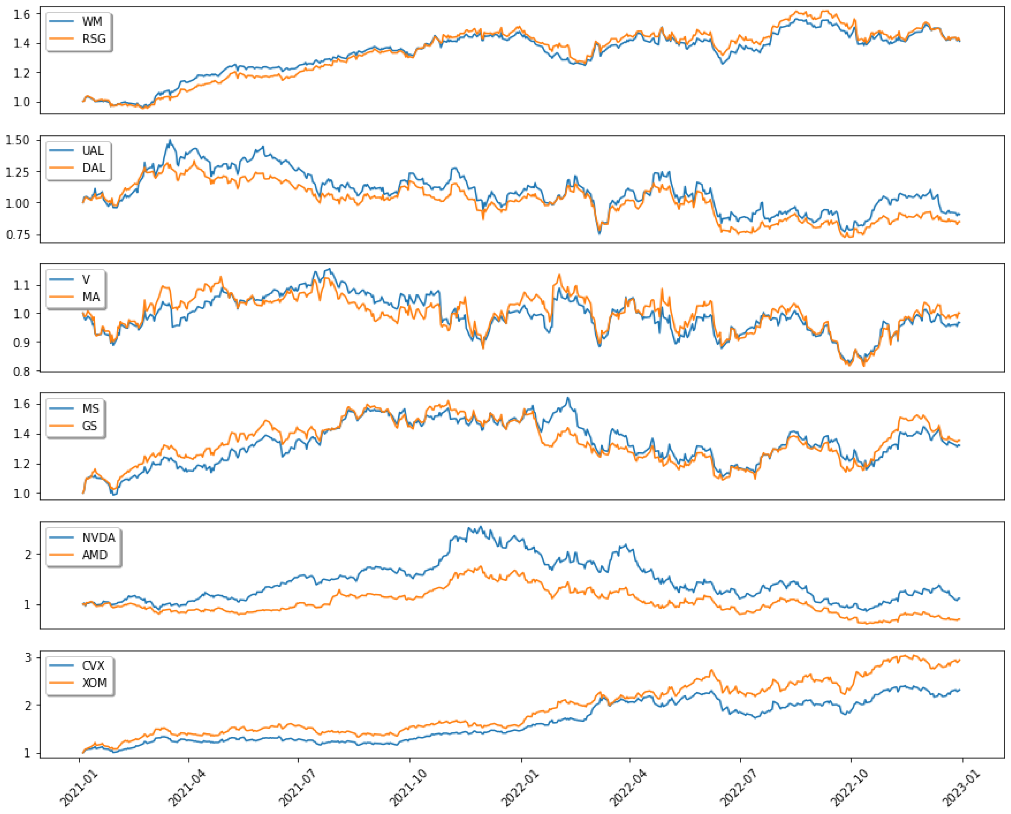
Table 2 provides a description of the companies, along with the ticker symbols of all the pairs: WM-RSG, UAL-DAL, V-MA, MS-GS, NVDA-AMD, and CVX-XOM.
For these six pairs, we collect the daily close prices for these stocks from 1 January 2021 to 31 December 2022 using the Yahoo! Finance API.
1 Figure 1 shows the price movements of each pair. Each price time series has been divided by its initial values for normalization. As we can see, the stock prices for each pair exhibit persistent comovement.
Pairs are constructed using the method detailed in
Section 3 and the daily adjusted close prices from the first year. In the experiment, the subsequent year is the trading period. In each quarter, data are used to generate new trading signals. With quarterly rebalancing, we test several trading thresholds and analyze annual performance statistics.
6.2. Trading on Each Pair
To demonstrate the efficacy of the proposed mean-reversion trading strategy, we first apply the strategy to six selected pairs separately. In the formation period, we use the data from 1 January 2021 to 31 December 2021 to compute the optimal ratio for each pair.
Table 3 lists the estimated best ratio and likelihood score of each pair. The parameters are selected as
,
,
, and
.
Then, we construct spreads from each pair based on the best ratio. In turn, each spread is traded in the trading period.
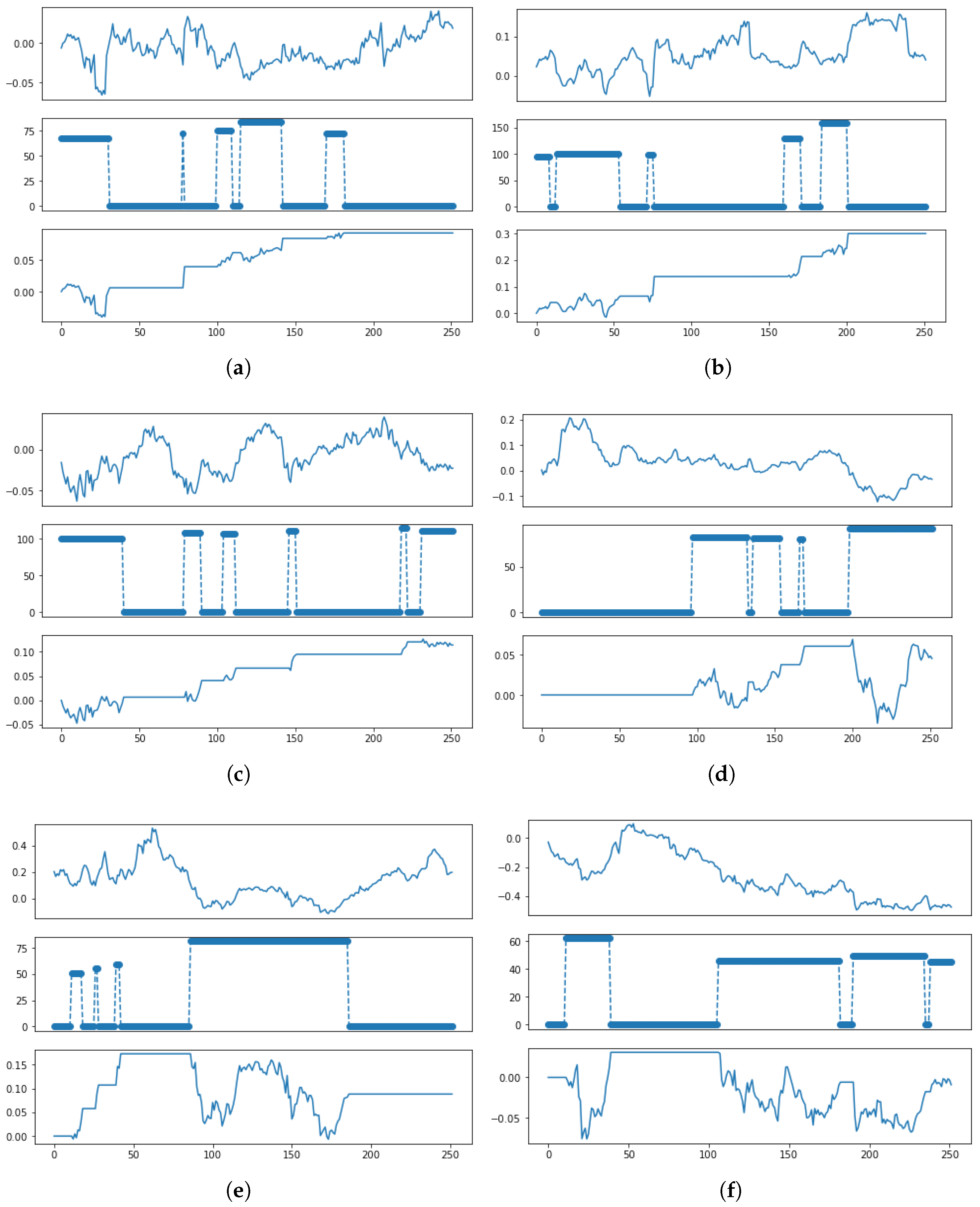
Figure 2 illustrates separately the spread, trading positions, and returns for the six pairs in 2022. From top to bottom in each panel, we record the movement of spread
, the position change
, and the cumulative return curve for each pair. As we can see, almost all of the pairs, except CVX-XOM, have positive annual profits, which demonstrates the effectiveness of the pairs trading strategy. As for the pair CVX-XOM, the main reason for failure is that the spreads constructed from the pairs do not display good mean reversion properties, as we can clearly observe a long-term downward trend in the spread. With this in mind, based on the spread behaviors and trading performance, it is intuitively optimal to allocate more weight to the first five pairs and less weight to CVX-XOM during the trading period. This echoes our motivation to propose a diversification framework to dynamically allocate weights on multiple pairs. It would be interesting to see whether any of the allocation methods can assign the weights accordingly.
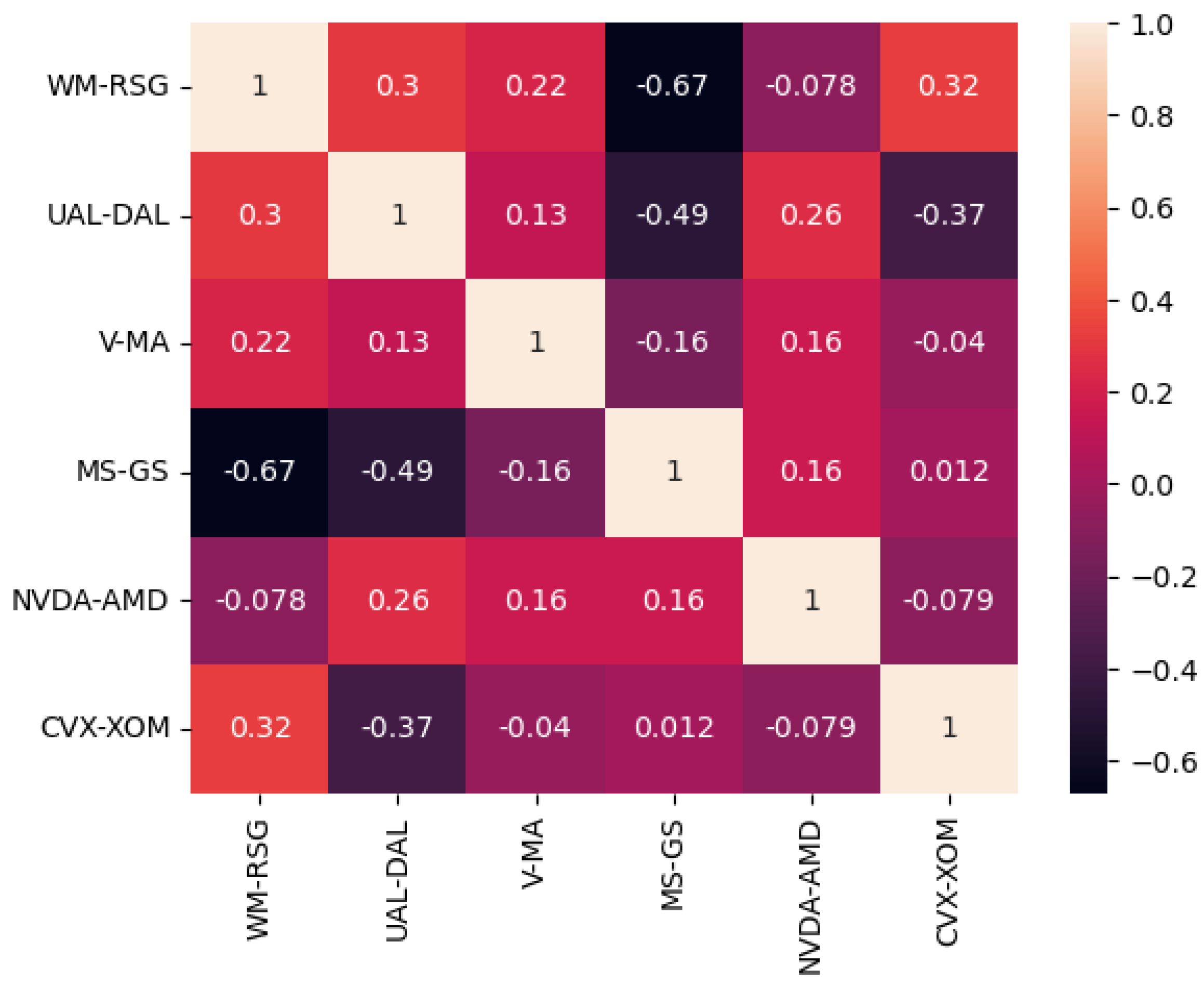
As shown in
Figure 3, the correlation coefficients between different spreads are generally small, with the most positive correlation coefficient being approximately 0.3. These low correlations suggest that there is a potential for diversification benefits in combining these spreads in a trading portfolio. By diversifying across multiple spreads, traders can potentially reduce portfolio volatility and increase the expected return. This motivates us to investigate the effectiveness of our proposed diversified trading framework.
6.3. Equal-Weight Portfolio
The baseline diversification is to trade all pairs equally, which means we implement the trading strategies for all pairs with equally allocated initial cash during the entire trading period. This equal-weight portfolio is conceptually the most straightforward way to create a diversified portfolio. It is included here to compare against nondiversified trading of single pairs and against other diversification methods.
To start, we first compare the performance of the equal-weight portfolio to the performance of every single pair in this section. The trading period is the year 2022, and the average annual and daily performance statistics of the trading strategies are presented in
Table 4. We consider different trading thresholds
. With a higher
K, the spread needs to deviate further from its moving average in order to trigger a trade. The criteria presented include daily return (DailyRet), daily standard deviation (DailyStd), daily Sharpe ratio (DailySR), annual maximum drawdown (AnnMDD), and annual cumulative PnL (AnnPnL). In this experiment, we observe that the equal-weight portfolio generally outperforms single pairs in terms of daily Sharpe ratio, daily standard deviation, and annual maximum drawdown. This indicates the effectiveness of diversification for mean reversion trading.
Moreover, we observe that the standard deviations of individual pairs range from 0.4 to 1, while the standard deviation of our portfolio is lower than 0.3. This indicates that the equal-weight portfolio strategy has a lower level of risk compared to the individual pairs. This can be attributed to the diversification effect, as the portfolio strategy involves trading multiple pairs simultaneously, which helps reduce the overall risk. Therefore, our results demonstrate that an equal-weight portfolio strategy can generate a higher return and achieve a lower level of risk through diversification.
6.4. Diversification Framework
We implement multiple mean reversion trading under the diversification framework using different allocation methods, and compare the performance with the baseline equal-weight portfolio. Since the trading period is one year (1/1/2022–12/31/2022) and the rebalancing window is set to be three months, the trading period is divided into four periods. As before, trading parameters are as follows: , days, days.
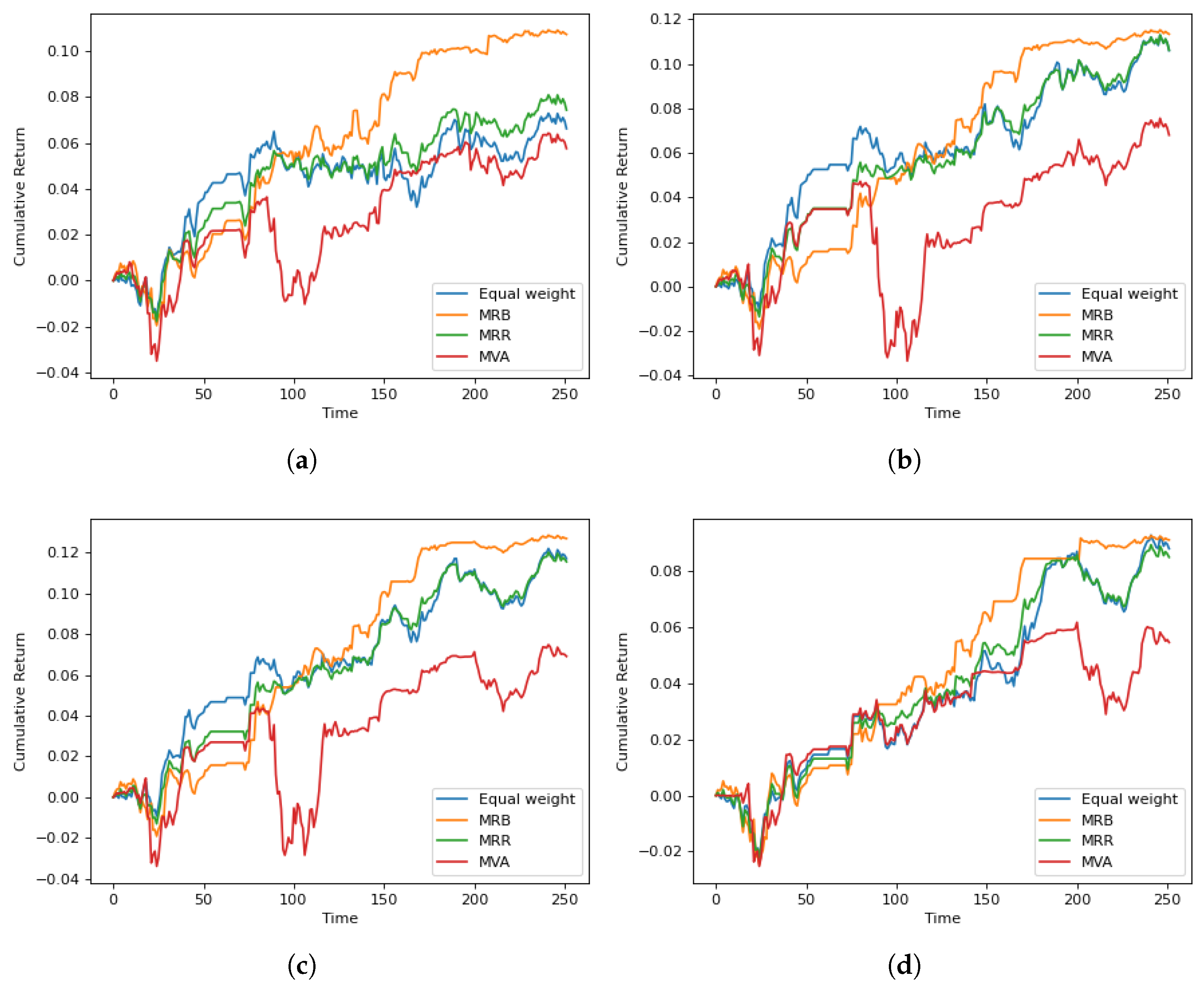
Figure 4 displays the cumulative return curves with different allocation methods in the year 2022. Here, “MRB” stands for the Mean Reversion Budgeting method, “MRR” represents the Mean Reversion Ranking method, and “MVA” refers to the portfolio generated by the mean-variance analysis. The equal-weight portfolio serves as a baseline portfolio for comparison.
In terms of cumulative returns, the MRB method outperforms the baseline portfolio by a significant margin. On the other hand, the MRR method’s returns are only slightly higher than the baseline. This is not surprising since the rank-based method tends to spread the weights more gradually from higher to lower-ranked pairs. In other words, the MRR method does not penalize the poorly fitted spreads severely and does not assign oversized weights to the spreads with the best mean-reverting properties.
However, taking volatility into account, subsequent experiments reveal that the ranking method achieves a higher Sharpe ratio than the baseline. In contrast, the MVA portfolio lags far behind the baseline. This is perhaps intuitive since the traditional mean-variance analysis does not take into account the mean-reverting properties of the spreads.
To provide a comparative analysis of different portfolio allocation methods versus the equal-weight portfolio, we summarize the statistics of trading performance with different thresholds in
Table 5. The statistics include daily returns (DailyRet), daily standard deviation (DailyStd), daily Sharpe ratio (DailySR), annual maximum drawdown (AnnMDD), and annual cumulative profit and loss (AnnPnL).
When compared to the baseline equal-weight portfolio, the MRB method significantly improves the annual return without increasing the standard deviation considerably. As a result, MRB yields a higher Sharpe ratio than the baseline portfolio. The MRR method significantly decreases volatility and also achieves a high Sharpe ratio. These observations support the notion that allocation based on mean reversion characteristics has the potential to improve portfolio performance.
Regarding the standard deviations of the differently weighted portfolios, it is notable that the MRR method exhibits the lowest standard deviation among all the portfolios, indicating that this particular combination of pairs is the least volatile. In addition, the MRB method also appears to decrease the standard deviation when compared to the equal weights and MVA methods. These findings provide further evidence for the advantages of employing a portfolio weights allocation approach to mitigate risk and enhance the overall performance of the portfolio.
6.5. MRB Portfolio Weights
In our experiment, the MRB method appears to be the best allocation method. In this section, we provide more details on how the weights vary under the MRB method during the trading period. Let us focus on the case where
.
Table 6 shows the estimated parameters using the data from 1 January 2022–31 December 2022. As we can see, the NVDA-AMD and CVX-XOM pairs have the lowest likelihood scores.
Table 7 shows the changes in portfolio weights for each quarter during that year. Notice that the weights for the NVDA-AMD and CVX-XOM pairs are close to zero. This is consistent with the MRB method where weights are proportional to the likelihood scores.
7. Conclusions
We have presented a trading program that dynamically allocates capital to multiple mean reversion trading strategies. The approach is designed for trading multiple pairs in order to achieve diversification effects. Moreover, the dynamic rebalancing is adaptive to the current model estimates and based on the relative performance or path behaviors of the pairs in the portfolio. Our empirical experiments have shown that, for a given set of pairs traded, the allocation method plays a significant role in the success of the diversification framework.
This paper provides portfolio managers and traders with a useful and flexible framework to test trading strategies and build portfolios involving multiple pairs. The approach discussed herein can also be applied to multiple futures spread trading that is common in other asset classes, such as interest rates, commodities, and currencies. There are plenty of examples of mean-reverting spreads between futures contracts in different markets, including Brent vs. WTI crude oil, soybean vs. soybean meal, gold vs. silver, and many more. Spread trading is very common in managed futures portfolios.
Future research directions include considering a risk-sensitive approach and incorporating additional risk controls into the trading problem. The effects on trading performance would be of practical interest. Another direction is to consider a variation of the mean-reverting model. In particular, regime-switching mean-reverting models have been used for futures trading (see
Leung and Zhou 2019) and they can be suitable here for multiple spread trading.


