A Compound Up-and-In Call like Option for Wind Projects Pricing

Abstract

Wind energy projects represent, currently, a valid opportunity to support United Nations Sustainable Development Goal 7. However, these projects can appear financially unattractive considering the unfavorable meteorological conditions, uncertain electricity market price, uncertain market demand, unpredictable project performance, riskiness of investment stages, etc. This paper provides a real options pricing model applied for the evaluation of a wind farm project to include the uncertainty that can affect future performance. The methodology proposed uses a compound call option model with two barriers applied, respectively, to the twofold phase framework that would act as a sort of up-and-in barrier. The compound call option model allows us to valuate the managerial flexibility to proceed with the following investment stages depending on the success of the previous ones and, through the barriers, the methodology gives the investor the opportunity to consider some profitability thresholds below, past which the investment should be abandoned. We develop a discrete case methodology by using the binomial approach. A hypothetical case study is shown to implement the theoretical framework by using likely data.

1. Introduction

Renewable energy projects have become very important considering the environmental problems that governments can face in the world. To solve these problems, all the United Nations Members States adopted in 2015 the 2030 Agenda for sustainable development that provides a plan related to people, the planet and prosperity. The 2030 Agenda focuses on 17 Sustainable Development Goals (SDGs) that refer to social issues such as ending poverty, equality challenges, peace, environmental, climate actions, etc. Specifically, the UN Sustainable Development Goal 7 aims to “ensure access to affordable, reliable, sustainable and modern energy for all”. Wind energy projects can support this goal.

The valuation of the wind investments should include their characteristics such as uncertainty and sequential decision-making. The uncertainty refers, for example, to the risks deriving from unpredictable market price conditions and from variable power production depending on the wind speed (Rodriguez et al. 2021). Considering this riskiness, it is important to include the managerial flexibility to change the investment decision (to abandon the project, to expand the size, etc.) in the project valuation. The classical static approaches based on discounted cash flows methods, such as the Net Present Value (NPV), cannot price the managerial flexibility (Ross 1995). For this reason, the Real Option Approach (ROA) has become one of the most diffused approaches to valuate uncertain projects (Trigeorgis 1993). In fact, the ROA allows us to capture the managerial flexibility, called “optionality”, to change investment decision depending on the variable market conditions and the project performance evolution. For example, Kellogg and Charnes (2000) adopted the ROA to value a biotechnology company through the binomial lattice model through the risk-neutral valuation of Cox et al. (1979). The idea is that some biotechnology companies could have a low value if the pricing happens at the early stage of development. This value could increase after a significant development of the project. Thus, the ROA is useful to valuate risky businesses whose value can change during the time. Lee (2011) showed that the real options methodology is a reliable approach to price the investment planning uncertainty in wind energy development.

The sequential decision-making refers to the multi-stage nature of these projects. Loncar et al. (2017) identified two main phases for wind projects: the first contains the investment to initiate, evaluate and design the wind farm projects; the second contains the investment to execute and operate. These two phases are not independent of each other but, conversely, the investor should proceed by investing in the following stages only if the previous ones are profitable. Otherwise, he should stop the investment process.

Previous studies faced the valuation of uncertain projects characterized by sequential nature considering them as compound options. Geske (1979) presented a model to price compound options that consist of options on options. He demonstrated that the Black and Scholes (1973) formula can be viewed as a special case of a compound options model. By extending the compound options logic to the real cases, we can talk about compound ROA. In a real scenario, the compound ROA is used to valuate multistage projects. For instance, Panayi and Trigeorgis (1998) analyzed the multistage or compound ROA for investment decisions in information-technology infrastructure and for investment decisions regarding a bank expansion of its operation into another country. Cassimon et al. (2004) and Hauschild and Reimsbach (2015) used the compound ROA to price R&D projects characterized by various phases and by a high level of uncertainty in each of them. Considering the riskiness of phases, Martinez-Cesena and Mutale (2012) used the ROA to valuate the wind power projects by embedding the uncertainty related to planning and design stages. They confirmed that the ROA tends to increase the project value by making them more attractive.

In addition to this, some studies added some profitability or default thresholds, also called barriers, to the classical ROA for monitoring various financial situations in the project valuation. The barrier options are a type of option in which the payoffs depend on whether or not the underlying asset price reaches or exceeds a pre-determined barrier price (Hull 2013). The application of the idea of the barrier options to the real cases generates the barrier ROA methodologies. For example, Engelen et al. (2016) included a down-and-out barrier into compound ROA to mitigate the default risk of the hydrogen fuel infrastructures, Di Bari (2021) applied the logic of the down-and-out barrier ROA to valuate public–private partnership projects and the use of barrier is justified to control possible moral hazardous behavior put into practice by private firms. Rodriguez et al. (2021) designed and evaluated an up-and-in barrier option applied to wind energy fields considering the variability in power production. The study of van Zee and Spinler (2014) embedded a down-and-out barrier option in the ROA to valuate R&D investments considering the public sector.

The barrier ROA can be developed in the continuous or discrete time depending on the project characteristics. Regarding the discrete time approaches, Reimer and Sandmann (1995) showed the methods to price various types of barrier approaches through the Cox et al. (1979) model. We differ from them by applying the methodology for renewable projects valuation and by adjusting the models for the characteristics of these projects, such as the multistage nature. In fact, although previous studies applied barrier options to valuate real projects, there is a lack of works that valuate a wind farm project taking into account the sequential decision-making nature by using the logic of the compound up-and-in options applied in the discrete time through a binomial approach. However, some works contribute successfully to combine barrier options with the compound options logic that can model multistage projects (Bufalo et al. 2022). For example, Liu et al. (2018) proposed a valuation of n-fold compound barrier options in continuous time focusing on the down-and-out case that, generally, is also proposed to control the default risk.

This work extends the real options literature in discrete time with the binomial model use. In fact, this paper contributes to the existing literature by providing an innovative valuation model based on the ROA that, through two barriers applied for two sequential stages, can control the riskiness of renewable projects. The methodology consists in a kind of compound called an up-and-in-like option model applied to price wind projects and to fit the renewable projects characteristics. This approach embeds the multi-stage nature through the compound options framework and mitigates the risk of financial losses by applying the logic of the up-and-in barrier options. The use of these barriers implies that, in the presence of two subsequent investments, the investor should make the second investment if in the previous stage the project evolution overcomes the costs and a certain threshold of revenues. This threshold is identified as a barrier needed to avoid unpredictable financial losses. In this way, the methodology tries to control the project riskiness. We also provide an example to show how to implement our approach. The results show that the project valuation through the compound up-and-in call-like option is higher than classical NPV approach. The paper is organized as follows: Section 2 describes the compound up-and-in call-like option model based on the binomial lattice model applied for a wind project valuation; Section 3 describes a case study by using likely data; and Section 4 provides conclusive remarks.

2. Methodology

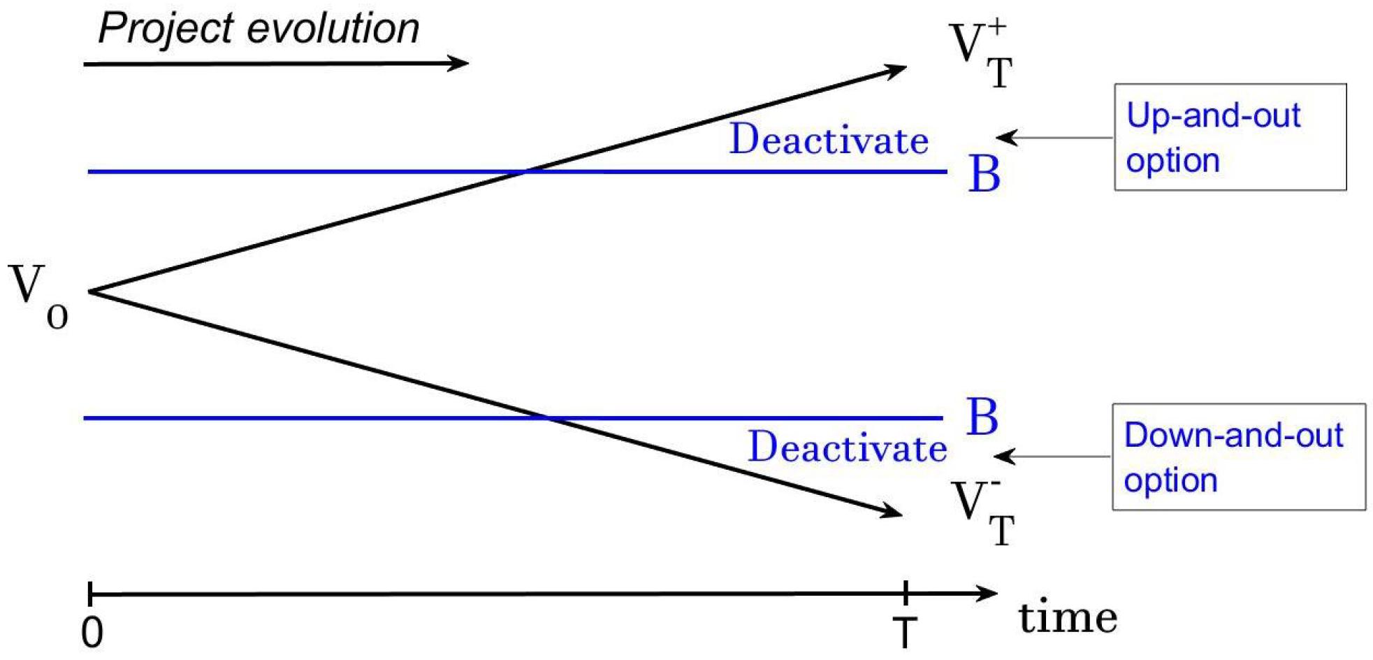
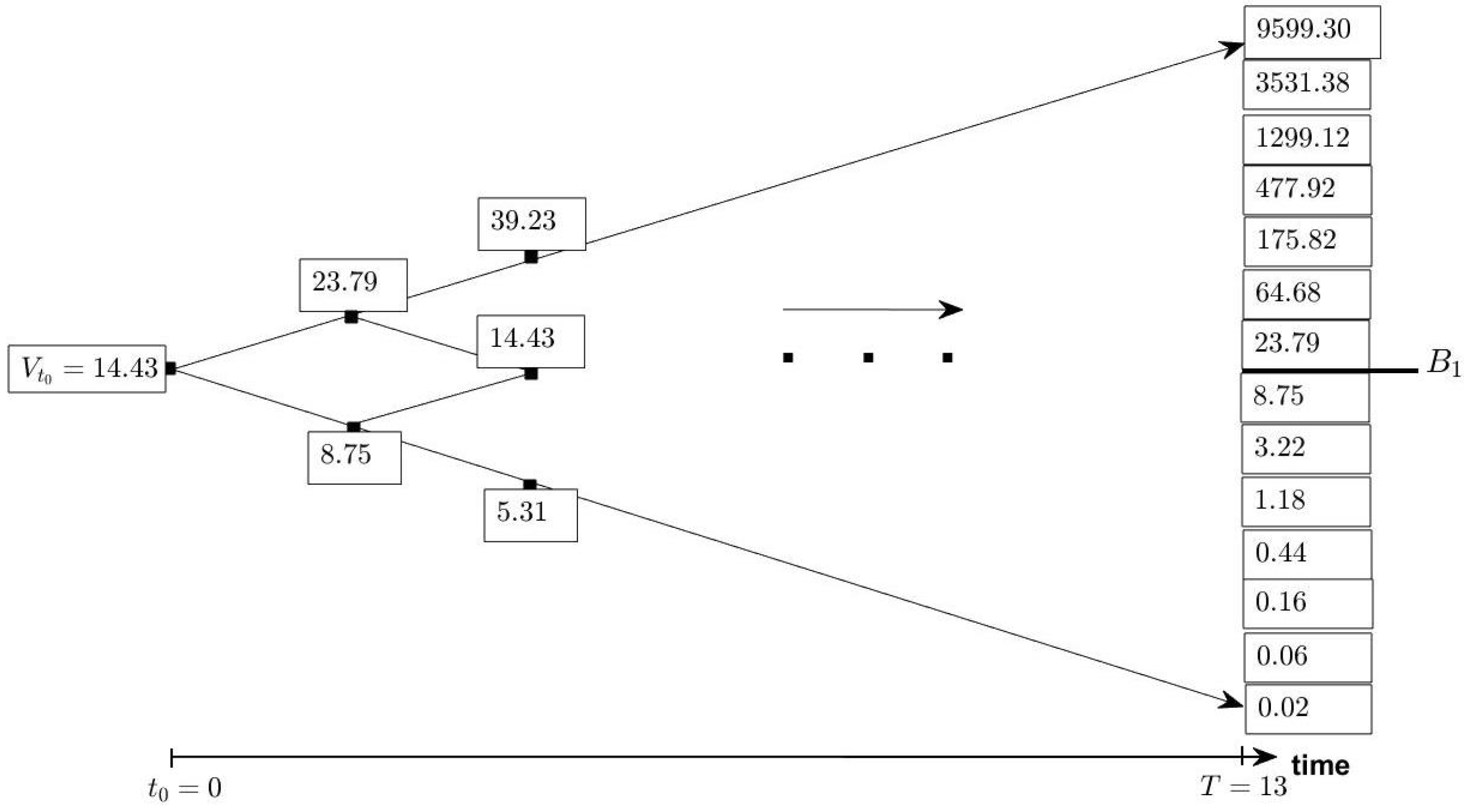
2.1. Up-and-In Option

The barrier options represent a particular case of financial options of which the right to be exercised depends on whether the underlying asset $V_t$ during its evolution in the period $t=0,\dots ,T$ intersects a certain level of threshold (B), called a barrier, or not (Hull (2013) and Soltes and Rusnakova (2013), just to name a few). We can divide the barrier options mainly into two categories: knock-out and knock-in options (Rambaud and Pérez 2016).

In the case of knock-out options, the right to be exercised vanishes if the underlying asset during its evolution intersects the barrier (see Figure 1). We denote $V_T^{+}=V_0·u$ and $V_T^{-}=V_0·d$, where u and d represent, respectively, the up and down movements that the underlying asset can make during its evolution. The knock-out options can be divided into up-and-out (options cease to exist if the underlying asset value exceeds the barrier), or down-and-out (options cease to exist if the underlying asset goes below the barrier).

In the case of knock-in options, the right to be exercised comes into existence if the underlying asset crosses the barrier (see Figure 2). These options can be divided into: up-and-in option (they are activated if the underlying asset exceeds the barrier), or down-and-in options (they are activated if the underlying asset value goes below the barrier). In general, we can state that the up-option model is characterized by $B>V_0$, and the down-option model is characterized by $B<V_0$ where $V_0$ represents the initial value of the underlying asset.

In this work, we use an up-and-in call-like option model that it is embedded in the compound real options mechanism to valuate the wind projects. We identify this approach as compound call up-and-in-like options model for the combination of a sort of up-and-in option with the compound real options logic that can consider the multi-stage nature of the wind projects.

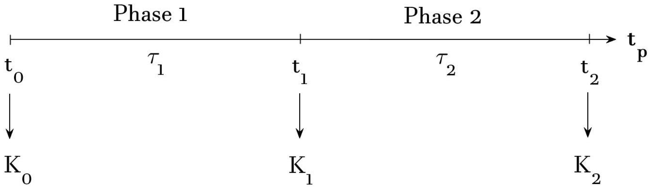
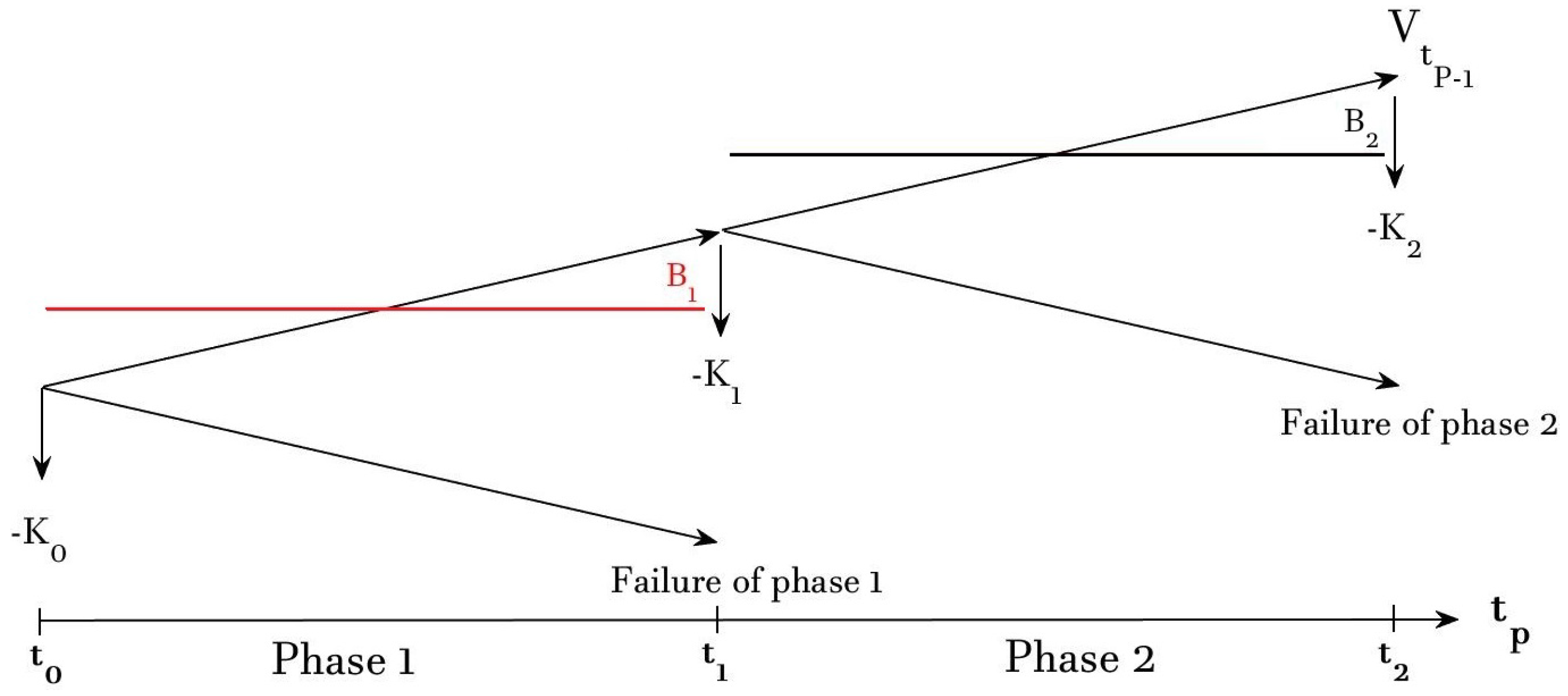
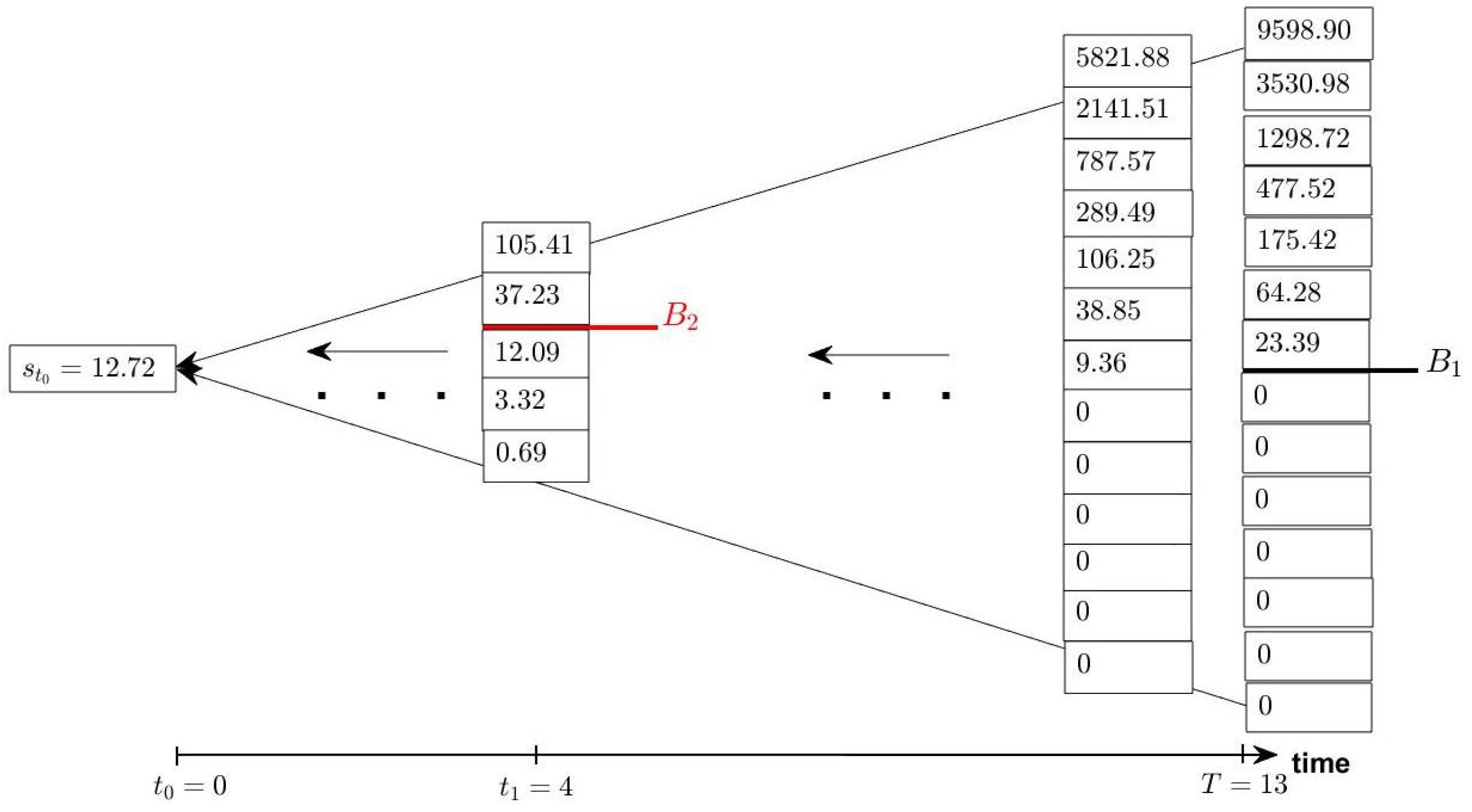
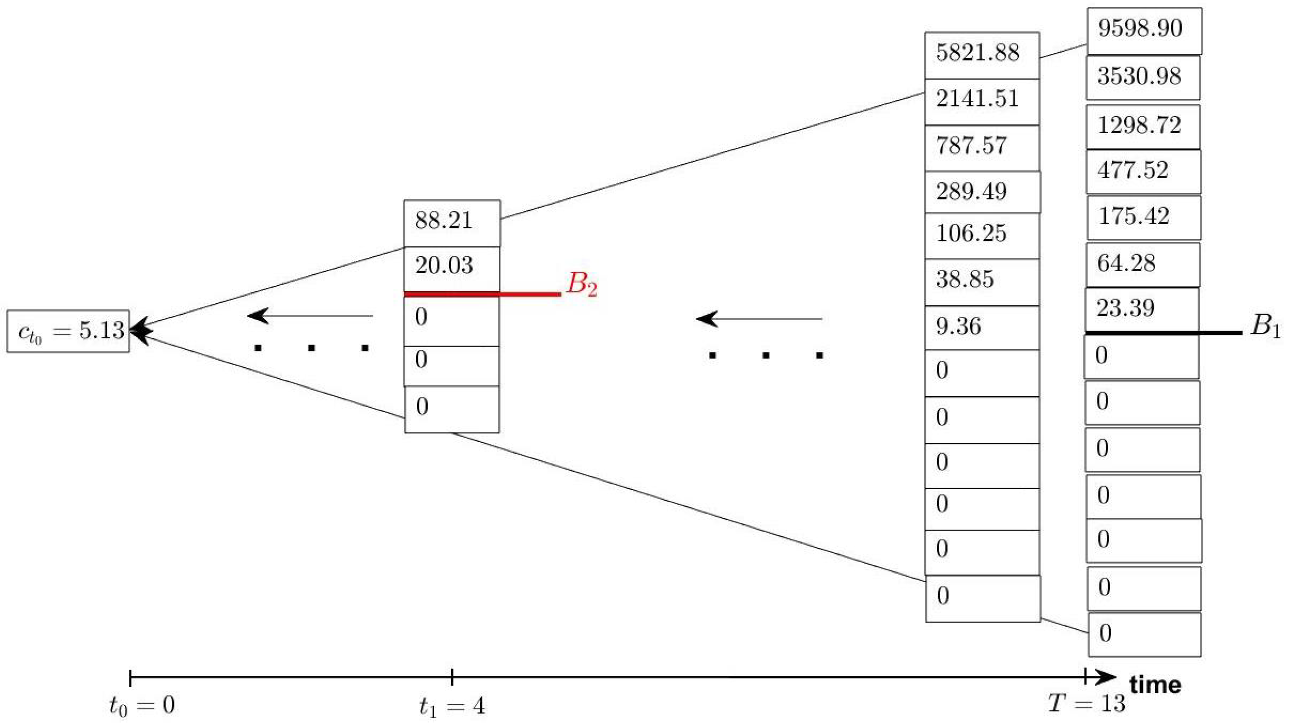
2.2. Compound Up-and-in-Like Option for Wind Projects Valuation

In this section, we explain the methodology to valuate wind farm projects considering their characteristics. These projects are risky investments considering the huge amount of irreversible capital required to pursue them (Venetsanos et al. 2002). Moreover, these investments are also characterized by sequential decision-making since they contain various phases (Loncar et al. 2017). Bufalo et al. (2022) showed that these projects mainly contain three sequential investments: the first for the wind farm planning, the second for the wind farm construction and the third to pursue the operating phase. The investor should recover these costs by selling the energy of the wind project. The project value corresponds with the discounted cash inflows of the project at time $t_0=0$, and so the present value, denoted by $V_{t_0}$.

We identify as P the phases with $p=0,\dots ,P-1$, where we set $P=3$ in our practical case. Hence, $p=0$ represents the first investment step to plan the project; $p=1$ represents the stage to build the wind farm and $p=2$ is the stage related to the operating activity. We denote the investments required for each step, respectively, by $K_0$, $K_1$, and $K_2$. Moreover, the length of each phase is denoted by ${\tau }_p=t_p-t_{p-1}$, where $t_p$ values represent the boundary deadline of each phase (see Figure 3). Thus, we consider two phases: the first one goes from $t_0$ to $t_1$, and the second one from $t_1$ to $t_2$. The final instant time $t_2$ in our case represents the maturity T. The barriers are applied at time $t_p$ by nullifying the nodes in which underlying asset values are lower than costs $K_p$ and barriers $B_p$. Once we found the values at time $t_p$ of the binomial tree, we adopt the simple backward procedure without giving the possibility to exercise the real option at time ${\tau }_p$. For this reason, we have a kind of European-style real option for each phase. The use of this setting is justified by the assumption that we assume the investor should wait the entire project evolution during the period of each stage before deciding to continue or not to continue with the next investment stage. Thus, we apply two up-and-in thresholds $B_p$ in this way: $B_2$ for the time $t_2$ and $B_1$ for the time $t_1$. In fact, in this model we do not use the classical barrier options pricing, which is a path-dependent pricing model (Glasserman 2003). We put the barrier only at the boundary deadline of each phase $t_p$ and the investor should consider only this time to choose whether to proceed or not with the next stage. These barriers act as two profitability thresholds that should guarantee the pursuit of investments $K_p$ only if there is a sufficient margin of revenues to face the potential unpredictable market changes, such as the changing electricity prices, the reduction of market demand, etc.

We set our model by applying the binomial method in the discrete time. Gaudenzi and Lepellere (2006) proposed a first version of pricing American barrier options through binomial tree, and we differ from them by creating a compound barrier options approach applied for real investments. The application of this approach in a real case generates a modified barrier option, which in our case does not contain the path-dependence characteristic typical of exotic financial options. Moreover, the setting of the compound options framework in the discrete time has been developed considering the work of Biancardi et al. (2021).

The analysis starts by analyzing the present value $V_{t_0}$ evolution.1 The present value acts as underlying asset and evolves as a binary random walk through two movements: up (u) and down (d) along the binomial lattice model with a risk-neutral probability2 $\mathbb{Q}=(q,1-q)$, with

$$q=\frac{(1+r_f)-d}{u-d}$$

(1)

where $r_f$ represents the risk free rate.

We start by applying the simple up-and-in call option model. We start from the final phase, $P-1$, at which the simple call up-and-in-like option (s) with the barrier $B_2$ assumes the following values:

$$s_{P-1}=\left\{\begin{array}{c}max\left[V_{t_{P-1}}-K_2;0\right]\mathrm{if}{V}_{t_{P-1}}\ge B_2\hfill \\ 0\mathrm{if}{V}_{t_{P-1}}<B_2\hfill \end{array}\right.$$

(2)

This means that the portfolio managers or financial analysts assume that the investor should invest $K_2$ if the project becomes profitable during its evolution ($V_{t_{P-1}}>K_2$), otherwise the investor should avoid to invest by obtaining 0. Moreover, this payoff is subject to another condition: the investment should be pursued only if the project value overcomes a certain threshold, i.e., barrier, of revenues ($V_{t_{P-1}}\ge B_2$) in order to guarantee a profit margin needed to face possible unpredictable market changes. The Equation (2) represents a general condition that we can explicate for each nodes of the binomial tree assuming that $n_p=0,\dots ,t_p$ represents the number of up movements along the binomial tree until the boundary deadline of each phase $t_p$; and $m_p=0,\dots ,{\tau }_p$ represents the up movements inside of each phase during the backward process. This is because we have denoted as ${\tau }_p=t_p-t_{p-1}$ the length of each phase and as $t_p$ the final time (boundary deadline) of each phase. A graphical exhibit to clarify this nomenclature is shown in Figure 3. Thus, considering that we denote as P the phases with $p=0,\dots ,P-1$ where $P=3$, we identify as $t_{P-1}=t_2$ and ${\tau }_{P-1}={\tau }_2$, respectively, the boundary deadline and the length of the second phase; and as $t_{P-2}=t_1$ and ${\tau }_{P-2}={\tau }_1$, respectively, the boundary deadline and the length of first phase.

Following the recent approach of Attalienti and Bufalo (2020, 2022), let us define

$$V_{n_p}^{{\rho }^{(p,n_p-p)}(u,d)}:=u^p·d^{n_p-p}·V_{t_0}$$

for any integer $p\in \{0,1,\dots ,n_p\}$, where ${\rho }^{(p,n_p-p)}(u,d)$ denotes any permutation with repetition of the $n_p$-tuple

$$(\underset{p}{\underbrace{u,\dots ,u}},\underset{n_p-p}{\underbrace{d,\dots ,d}}),$$

and corresponds to choosing p “up moves” (and $n_p-p$ “down moves”) for a total of $\left(\genfrac{}{}{0pt}{}{n_p}{p}\right)$ different nodes in the tree.

So, we can depict Equation (2) for each node as follows:

$$\begin{array}{c}{s}_{P-1}^{{\rho }^{(n_{P-1},t_{P-1}-n_{P-1})}(u,d)}=\hfill \\ \left\{\begin{array}{c}max\left[V_{t_0}·u^{n_{P-1}}·d^{t_{P-1}-n_{P-1}}-K_2;0\right]\mathrm{if}{V}_{t_0}·u^{n_{P-1}}·d^{t_{P-1}-n_{P-1}}\ge B_2\hfill \\ 0\mathrm{if}{V}_{t_0}·u^{n_{P-1}}·d^{t_{P-1}-n_{P-1}}<B_2\hfill \end{array}\right.\hfill \end{array}$$

(3)

where $t_0=0$.

At this point, the analysis proceeds by backward induction until $P-2$, by calculating $\tilde{s}$ that represent the values at time $\tau$:

$${\tilde{s}}_{P-1}^{{\rho }^{(n_{P-2},t_{P-2}-n_{P-2})}(u,d)}=V_{n_{P-2}}·\Phi (\tilde{q},{\tau }_{P-1},{\alpha }_{P-1})-\frac{K_2}{{(1+r_f)}^{{\tau }_{P-1}}}·\Phi (q,{\tau }_{P-1},{\alpha }_{P-1})$$

(4)

where

$$\Phi (q,{\tau }_{P-1},{\alpha }_{P-1}):=\sum _{m_{P-1}={\alpha }_{P-1}}^{{\tau }_{P-1}}\left(\genfrac{}{}{0pt}{}{{\tau }_{P-1}}{m_{P-1}}\right)·q^{m_{P-1}}·{(1-q)}^{{\tau }_{P-1}-m_{P-1}}$$

is the so-called complementary binomial distribution, ${\alpha }_{P-1}$ being the minimum number of upward moves necessary for the process $V_t$ to be greater than $max\{K_2,B_2\}$ at time ${\tau }_{P-1}$. Moreover, the measure $\tilde{\mathbb{Q}}=(\tilde{q},1-\tilde{q})$ represents the risk measure $\mathbb{Q}$ under the numèraire $V_t$. More precisely, according to Attalienti and Bufalo (2020), it holds

$$\tilde{q}=\frac{uq}{1+r_f}.$$

At time $P-2$, the value of the simple up-and-in call-like option becomes the new underlying value to which the investor should subtract the capital required to pursue the phase $P-2$. In this way, we have a sort of option on another option (compound option) that allows us to capture the managerial flexibility to proceed with the following investment only if the economical conditions of the previous one is profitable. This profitability is evaluated by considering the passing of a new barrier $B_1$. Thus, this new condition is represented by:

$$c_{P-2}=\left\{\begin{array}{c}max\left[{\tilde{s}}_{P-1}-K_1;0\right]\mathrm{if}{\tilde{s}}_{P-1}\ge B_1\hfill \\ 0\mathrm{if}{\tilde{s}}_{P-1}<B_1\hfill \end{array}\right.$$

(5)

The explicit formula of Equation (5) for each node is:

$$\begin{array}{c}{c}_{P-2}^{{\rho }^{(n_{P-2},t_{P-2}-n_{P-2})}(u,d)}=\hfill \\ \left\{\begin{array}{c}max\left[{\tilde{s}}_{P-1}^{{\rho }^{(n_{P-2},t_{P-2}-n_{P-2})}(u,d)}-K_1;0\right]\mathrm{if}{\tilde{s}}_{P-1}^{{\rho }^{(n_{P-2},t_{P-2}-n_{P-2})}(u,d)}\ge B_1\hfill \\ 0\mathrm{if}{\tilde{s}}_{P-1}^{{\rho }^{(n_{P-2},t_{P-2}-n_{P-2})}(u,d)}<B_1\hfill \end{array}\right.\hfill \end{array}$$

(6)

The analysis proceeds by backward induction until $P-3$ as described by Biancardi et al. (2021):

$$\begin{array}{c}{\displaystyle {\tilde{c}}_{P-2}^{{\rho }^{(n_{P-3},t_{P-3}-n_{P-3})}(u,d)}=}\hfill \\ \frac{{\displaystyle \sum _{m_{P-2}=0}^{{\tau }_{P-2}}\left(\genfrac{}{}{0pt}{}{{\tau }_{P-2}}{m_{P-2}}\right)·q^{m_{P-2}}·{(1-q)}^{{\tau }_{P-2}-m_{P-2}}·c_{P-2}^{{\rho }^{(n_{P-3}+m_{P-2},t_{P-3}-n_{P-3}-m_{P-2}})(u,d)}}}{{(1+r_f)}^{{\tau }_{P-2}}}\hfill \end{array}$$

(7)

In our analysis, ${\tilde{c}}_{P-2}$ represents the project value at time $t_0=0$, also called $c_0$, to which it should be subtract the investment that is required to initiate the actual wind farm project by planning it, $K_0$. This investment represents the cost to start the entire project process that should be make regardless of the profitability thresholds. Thus, the project valuation ($PV$) at time $t_0$ is equal to:

$$P{V}_{t_0}=-K_0+c_{t_0}$$

(8)

The result of this subtraction represents the project valuation considering a double threshold, the first one between $t_0$ and $t_1$ and the second one between $t_1$ and $t_2$, above which the investment is assumed to be profitable in order to allow the investor to proceed with the following investment phase. In fact, the compound options logic allows us to price the managerial flexibility to proceed with the following investment stage only if the previous one is successful. Conversely, if the previous phases present a failure, the investor should stop the investment process without proceeding with the next investment. Therefore, the investor should make the second investment $K_2$ only if the underlying asset evolution in the first stage is higher than first cost $K_1$ and $B_1$; otherwise, the investor should not invest by obtaining zero rather than a financial loss. In real options valuation, the capital required for each stage acts as strike prices that are paid to obtain project revenues considering the managerial flexibility value. This flexibility consists in the active management value of investing only if the renewable project value becomes higher than the costs, and, at the same time, than some profitability thresholds or barriers. A graphical exhibit of the backward induction process in the compound call up-and-in real option is shown in Figure 4.

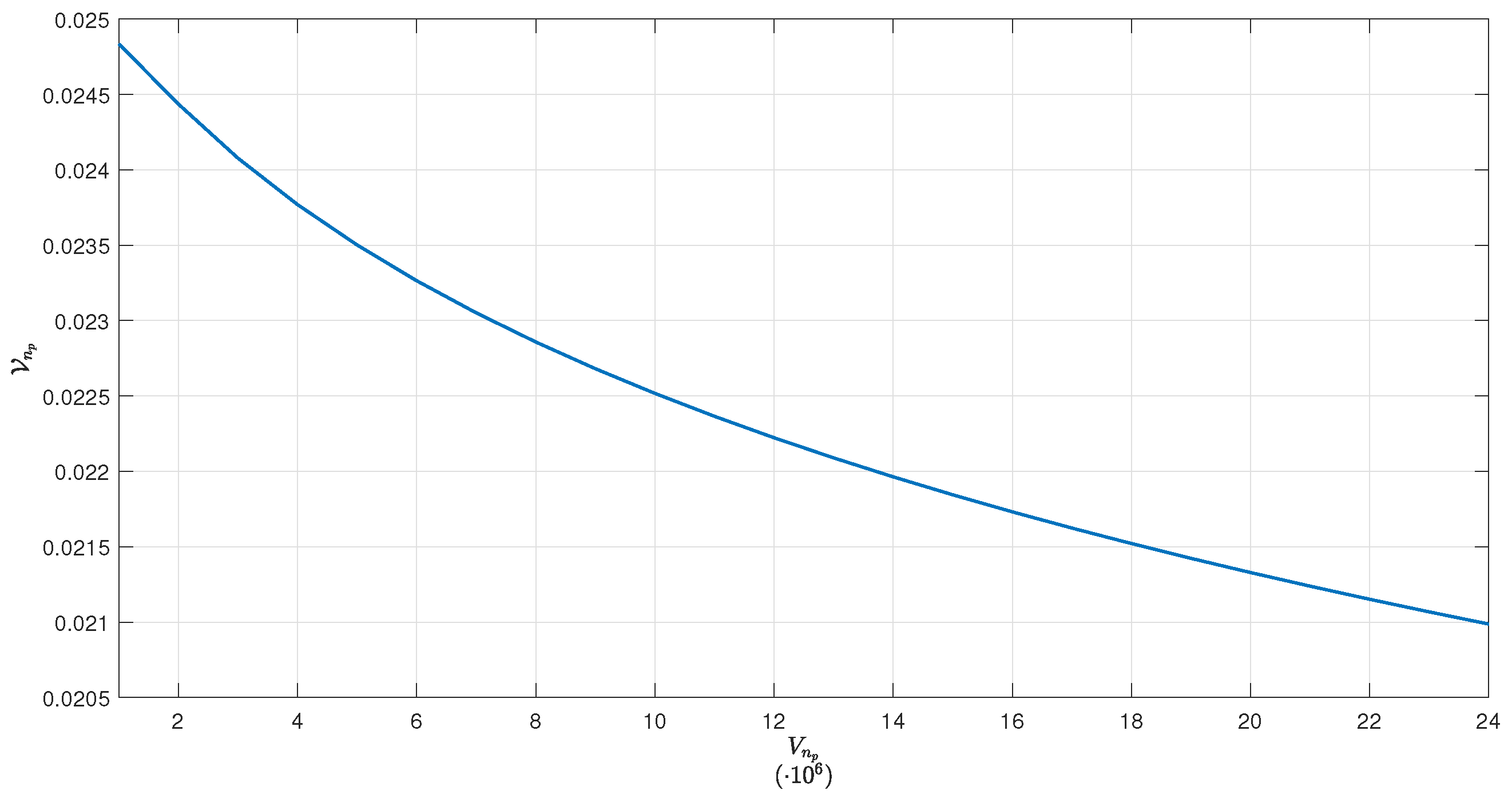
2.3. Valuation of Vega

As it is well known, renewable output is very intermittent, hard to predict, and increases market volatility. For this reason, the computation of the Greek Vega may be helpful to measure the sensitivity of volatility. In order to compute the Vega $\mathcal{V}$, we use the notation of Cox et al. (1979), by setting

$$u=e^{\sigma \sqrt{\Delta }},d=\frac{1}{u},q=\frac{e^{r\Delta }-d}{u-d}$$

where $\Delta$ is a time-step, and consider the increments $n_p$ as $p\Delta$, as it is commonly done in financial applications. Now, by following Muroi and Suda (2017), the Vega (at step $n_p$) may be computed by the recursive backward algorithm

$${\mathcal{V}}_{n_p}\left(\sigma \right)={\mathbb{E}}^{\mathbb{Q}}\left[-e^{-r-f\Delta }\left(1+\frac{2r_f}{{\sigma }^2}\right)\left(\frac{{\epsilon }_{p+1}-\mu \Delta }{2}\right){\mathcal{S}}_{n_p+1}\left(V_{n_p}{e}^{\sigma {\epsilon }_{p+1}}\right)\right]+$$

$${\mathbb{E}}^{\mathbb{Q}}\left[e^{-r_f\Delta }{\mathcal{D}}_{n_p+1}\left(V_{n_p}{e}^{\sigma {\epsilon }_{p+1}}{\epsilon }_{p+1}\right)V_{n_p}{e}^{\sigma {\epsilon }_{p+1}}{\epsilon }_{p+1}\right]+{\mathbb{E}}^{\mathbb{Q}}\left[e^{-r_f\Delta }{\mathcal{V}}_{n_p+1}\left(\sigma \right)\right]$$

(9)

where

$${\mathcal{S}}_{n_p}\left(V_{n_p}{e}^{\sigma {\epsilon }_{p+1}}\right)=e^{-r_f\Delta }{\mathbb{E}}^{\mathbb{Q}}\left[{\mathcal{S}}_{n_p+1}\left(V_{n_p}{e}^{\sigma {\epsilon }_{p+1}}\right)\right]$$

(10)

being ${\mathcal{S}}_{n_{P-1}}$ the payoff of the (simple) option defined in (3),

$${\mathcal{D}}_{n_p}\left(V_{n_p}{e}^{\sigma {\epsilon }_{p+1}}{\epsilon }_{p+1}\right)=\frac{{\mathcal{S}}_{n_p+1}\left(V_{n_p}u\right)-{\mathcal{S}}_{n_p+1}\left(V_{n_p}d\right)}{2V_{n_p}\sigma \sqrt{\Delta }}$$

(11)

is the Greek Delta. Moreover, ${\left({\epsilon }_p\right)}_{p\ge 0}$ are i.i.d. random variables such that $\mathbb{P}({\epsilon }_p=\pm \sqrt{\Delta })=\mathbb{Q}$ and $\mu =\frac{1}{\sigma }\left(r_f-\frac{{\sigma }^2}{2}\right)$.

Figure 5 displays the Vega ${\mathcal{V}}_{n_p}\left(\sigma \right)$ for the “in the money” case, when the parameters are chosen according the case study of Section 3. As one may expect, the sensitivity of volatility decreases as the underlying process $V_{n_p}$ increases.

3. Case Study

In this section, we provide a case study in which we consider an investment in a wind farm project of 15 MW that consists in five wind turbine generators (WTG) of 3.00 MW. The yearly power generation of this project is assumed to be equal to 34,164 MWh.3 We lead our analysis over 13 years where $t_0=0$, $t_1=4$, and $t_2=13$. Note that in our case the time $t_2$ corresponds to the maturity T. The total capital required to pursue this project is assumed to be EUR 20 million divided as follows: the investment for planning $K_0$ is the 12% of the total cost, so equal to EUR 2.4 million; the investment for building the wind farm $K_1$ corresponds to the 86% of the total cost, so equal to EUR 17.2 million; and the investment for operating activity $K_2$ is equal to 2% of total investment and so equal to EUR 0.4 million.4

We expect the investor should recover the capital required to pursue the project by the revenues deriving from the Feed in Tariffs (FiT) mechanism5 that in this case it is assumed to be equal to 92.00 EUR/MWh.6 By multiplying 92.00 EUR/MWh by the yearly power generation (34,164 MWh), we can calculate the yearly revenues equal to EUR 3.143088 million that are assumed to be constant during the time. At this point, we can calculate the present value $V_{t_{P-3}}=V_0=€ 14.43$ million through the discounted cash flows analysis assuming a discount rate equal to 8%.7 

Table 1. Discounted cash flows approach.

Years	0	1	2	3	4	5	6	7	8	9	10	11	12	13
Revenues						3.14	3.14	3.14	3.14	3.14	3.14	3.14	3.14	3.14
Costs	−2.4				−17.2									0.4

shows all the cash flows required to calculate the static NPV in terms of million of EUR.

The results of the classical NPV would imply the rejection of the project since it shows a negative value $NPV=-€ 0.7576$ million. However, as explained in the Introduction, the NPV could lead to the wrong investment decision since it is not able to consider the managerial flexibility and the sequential decision making. Once we showed the static discounted cash flows analysis, we implement the compound call up-and-in-like option for the wind farm valuation. The final project value through the methodology cannot be assessed through a unique backward induction process and we will describe the process step by step by considering $\sigma =0.5$,8 $B_2=€ 15$ million, and $B_1=€ 14$ million. Firstly, we calculate the project value evolution $V_{t_p}$ following the up (u) and down (d) movements and we identify the option values below the barrier $B_2$ (see Figure 6).9

Secondly, we evaluate the binomial tree of the simple up-and-in call-like option $s_{t_p}$ by nullifying the values at the nodes below the barrier. We proceed backward and by adopting a risk-free rate $r_f=4\%$10 and $\Delta t=1$. Figure 7 shows the simple up-and-in call-like option calculated at time $t_0$.11 In this tree, we identify the new barrier $B_1$ put at time $t_1$ in red.

Then, we create another binomial lattice model for the compound call up-and-in-like option valuation. Figure 8 contains the values of simple up-and-in options $s_{t_p}$ given by Figure 7 from $t_2$ to $t_1$ that is the time instant in which the values of ${\tilde{s}}_2$ become the new underlying asset values. At time $t_1$, we apply Equation (6) and we nullify the values below the new barrier $B_1$. Then, we proceed backward until $t_0$ in order to calculate $c_0$ by using Equation (7). At this point, by applying Equation (8), we price the final project valuation that is equal to:

$$P{V}_{t_0}=-K_0+c_{t_0}=-2.4+5.13=€ 2.73 \mathrm{million}$$

Discussion of Results: Findings and Implications

The results show that the compound up-and-in call-like option methodology tends to appreciate the wind farm investment valuation since the project valuation presents a quite high positive value. This means that the project valuation at time $t_0=0$, controlling the uncertainty through two barriers, and considering the sequential decision-making nature, is $€ 2.73$ million. According to this approach, the portfolio managers or financial analysts should suggest that the investor pursue the wind farm project. The important finding is that the classical NPV approach would have led the investor to reject the investment decision, differently from the methodology based on the up-and-in-like options model proposed in this paper. In fact, the classical NPV valuation underestimates the project value by giving a negative result, which would have implied the rejection of the project. In fact, Panayi and Trigeorgis (1998) showed that traditional discounted cash flow approaches often ignore the active management deriving from the managerial flexibility pricing. Conversely, our compound up-and-in call-like option model allows the portfolio manager or financial analyst to make an assessment of the wind farm project by including the managerial flexibility value in an innovative way. The difference between the two approaches is relevant since $NPV=-€ 0.7576$ million and $P{V}_{t_0}=€ 2.73$ million. The methodology proposed in this work increases the project valuation by EUR 3.48 million.12

The methodology proposed in this work highlights the financial profitability by letting the wind farm projects appear attractive to potential investors. This does not mean that the NPV is useless. Conversely, the NPV can be successfully used to valuate projects that are not influenced by uncertainty and operational flexibility value. The need to have a methodology that can support renewable investment decisions is crucial to attract funds by private and public investors that, by increasing the number of renewable energy projects, would be in line with UN Sustainable Development Goal 7.

4. Conclusions and Limitations

This paper provides a methodology based on the compound call up-and-in-like option to valuate the wind farm projects. This innovative approach allows us to include the wind farm characteristics by considering their uncertainty and multi-stage nature. Moreover, the up-and-in barriers included in the model allow the portfolio managers who are in charge of investments or financial analysts to face in a proper way the riskiness of the wind farm projects by ensuring some certain revenue thresholds, i.e., barriers, at each investment phase. Thus, we embed in the methodology the possibility to proceed with the next investments only if the previous ones are profitable by exceeding a certain threshold of revenues. We also provide a case study that confirms that the compound call up-and-in-like option tends to appreciate the renewable projects without underestimating them. The methodology could be used as a valuation tool by switching our hypothetical assumptions for others that could refer to others real-world scenarios. The case study we proposed gives just an idea about how to implement our methodology, but the assumptions can be changed following the future renewable contexts. The findings of this work highlight the importance of a reliable methodology to price the renewable projects in order to make the portfolio managers or financial analysts conscious of the financial advantages of these investments. By attracting new investors and by increasing the number of renewable projects, this methodology could spur the pursuit of UN Sustainable Development Goal 7, which aims to spread the sustainable and modern energy for all people. Thus, by highlighting the project profitability, a potential investor could be interested in renewable project without necessarily needing very strong incentives.

This work presents some limitations. First, we use a revisited version of the barrier real option approach without applying the standard path-dependent setting in the continuous time. This is because it better fits our renewable case assumptions, but further research could extend our approach by overcoming this limitation. Second, we do not make a study regarding the wind intensity in our approach. We consider a general volatility parameter of revenues that explains that the revenues can change during the time for various reasons, including uncertain meteorological conditions, unpredictable consumer demand, etc. A deeper study can split various types of volatility and could focus on the flexibility in use following the wind blow uncertainty. In fact, the renewable projects may not always be economically exercised. Third, in this work, we do not address the problem to obtain more information about government behavior in terms of renewable energy support policies and incentive prices to decide more consciously whether to invest or not to invest. The information considered in the model refers to the transition of the investment process from the previous stage to the following one, since our methodology allows us to capture the managerial flexibility of proceeding with the second investment only if the previous one is successful. Future works could address an innovative model that can capture information about government behavior or incentive prices to valuate renewable project. In fact, from a policy perspective, the most important implication is with regard to how governments incentivize renewable energy. Fourth, our case study employs data borrowed from the related literature. However, by changing the data, the results can also vary. Further research could address a real-world case study in order to improve the practicability of the methodology.

References

1. Attalienti, Antonio, and Michele Bufalo. 2020. Option pricing formulas under a change of numèraire. Opuscula Mathematica 40: 451–73. [Google Scholar] [CrossRef]
2. Attalienti, Antonio, and Michele Bufalo. 2022. Expected vs. real transaction costs in European option pricing. Discrete and Continuous Dynamical Systems—Series S 15: 3517–39. [Google Scholar] [CrossRef]
3. Biancardi, Marta Elena, Antonio Di Bari, and Giovanni Villani. 2021. R&D investment decision on smart cities: Energy sustainability and opportunity. Chaos, Solitons and Fractals 153: 111554. [Google Scholar]
4. Black, Fischer, and Myron Scholes. 1973. The pricing of options and corporate liabilities. Journal of Political Economy 81: 637–54. [Google Scholar] [CrossRef]
5. Bufalo, Michele, Antonio Di Bari, and Giovanni Villani. 2022. Multi-stage real option evaluation with double barrier under stochastic volatility and interest rate. Annals of Finance 18: 247–66. [Google Scholar] [CrossRef]
6. Cassimon, Danny, Peter Jan Engelen, L. Thomassen, and Martine Van Wouwe. 2004. The valuation of a NDA using a 6-fold compound option. Research Policy 33: 41–51. [Google Scholar] [CrossRef]
7. Cox, John C., Sthephen A. Ross, and Mark Rubinstein. 1979. Option pricing: A simplified approach. Journal of Financial Economics 7: 229–63. [Google Scholar] [CrossRef]
8. Di Bari, Antonio. 2021. A barrier real option approach to evaluate public-private partnership projects and prevent moral hazard. SN Business & Economics 1: 43. [Google Scholar]
9. Engelen, Peter Jan, Clemens Kool, and Ye Li. 2016. A barrier options approach to modeling project failure: The case of hydrogen fuel infrastructure. Resources and Energy Economics 43: 33–56. [Google Scholar] [CrossRef]
10. Gaudenzi, Marcellino, and Maria Antonietta Lepellere. 2006. Pricing and hedging american barrier options by a modified binomial method. International Journal of Theoretical and Applied Finance 9: 533–53. [Google Scholar] [CrossRef]
11. Geske, Robert. 1979. The valuation of compound options. Journal of Financial Economics 7: 63–81. [Google Scholar] [CrossRef]
12. Glasserman, Paul. 2003. Monte Carlo Methods in Financial Engineering. New York: Springer. [Google Scholar]
13. Hauschild, Bastian, and Daniel Reimsbach. 2015. Modeling sequential R&D investment: A binomial compound option approach. Business Research 8: 39–59. [Google Scholar]
14. Hull, John C. 2013. Fundamentals of Futures and Option Markets, 8th ed. Englewood Cliffs: Prentice Hall. [Google Scholar]
15. Jouini, Elyès, Clotilde Napp, and Walter Schachermayer. 2005. Arbitrage and state price deflators in a general intertemporal framework. Journal of Mathematical Economics 41: 722–34. [Google Scholar] [CrossRef]
16. Kellogg, David, and John M. Charnes. 2000. Real-options valuation for a biotechnology company. Financial Analysts Journal 56: 76–84. [Google Scholar] [CrossRef]
17. Lee, Shun Chung. 2011. Using real option analysis for highly uncertain technology investments: The case of wind energy technology. Renewable and Sustainable Energy Reviews 15: 4443–50. [Google Scholar] [CrossRef]
18. Liu, Yu-hong, I-Ming Jiang, and Li-chun Chen. 2018. Valuation of n-fold compound barrier options with stochastic interest rates. Asia Pacific Management Review 23: 169–85. [Google Scholar] [CrossRef]
19. Loncar, Dragan, Ivan Milovanovic, Biljana Rakic, and Tamara Radjenovic. 2017. Compound real options valuation of renewable energy projects: The case of a wind farm in Serbia. Renewable and Sustainable Energy Reviews 75: 354–67. [Google Scholar] [CrossRef]
20. Martinez-Cesena, Eduardo Alejandro, and Joseph Mutale. 2012. Wind power projects planning considering real options for the wind resource assessment. IEEE Transactions on Sustainable Energy 3: 158–66. [Google Scholar] [CrossRef]
21. Muroi, Yoshifumi, and Shintaro Suda. 2017. Computation of Greeks using binomial tree. Journal of Mathematical Finance 7: 597–623. [Google Scholar] [CrossRef]
22. Ouelega, Bell Fanon. 2013. State-Price Deflators and Risk-Neutral Valuation of Life Insurance Liabilities. Technical Report. Association of African Young Economists. [Google Scholar]
23. Panayi, Sylvia, and Lenos Trigeorgis. 1998. Multi-stage real options: The cases of information technology infrastructure and international bank expansion. The Quartely Review of Economics and Finance 38: 675–92. [Google Scholar] [CrossRef]
24. Rambaud, Salvador Cruz, and Ana María Sánchez Pérez. 2016. Valuation of Barrier Options with the Binomial Pricing Model. Ratio Mathematica 31: 25–35. [Google Scholar]
25. Reimer, Matthias, and Klaus Sandmann. 1995. A Discrete Time Approach for European and American Barrier Options. Working Paper. Bonn: Department of Statistics, Rheinische-Friedrich-Wilhelms-Universität Bonn. [Google Scholar]
26. Rodríguez, Yeny E., Miguel A. Pérez-Uribe, and Javier Contreras. 2021. Wind put barrier options pricing based on the nordix Index. Energies 14: 1177. [Google Scholar] [CrossRef]
27. Ross, Stephen A. 1995. Uses, Abuses and Alternatives to the Net-Present-Value Rule. Financial Management 24: 96–102. [Google Scholar] [CrossRef]
28. Soltes, Vincent, and Martina Rusnakova. 2013. Hedging against a price drop using the inverse vertical ratio put spread strategy formed by barrier options. Engineering Economics 24: 18–27. [Google Scholar] [CrossRef]
29. Trigeorgis, Lenos. 1993. Real Options and Interactions with Financial Flexibility. Financial Management 22: 202–24. [Google Scholar] [CrossRef]
30. van Zee, Roger D., and Stefan Spinler. 2014. Real option valuation of public sector R&D investments with down-and-out barrier option. Technovation 34: 477–84. [Google Scholar]
31. Venetsanos, Kostantinos, Penelope Angelopoulou, and Theocharis Tsoutsos. 2002. Renewable energy sources project appraisal under uncertainty—The case of wind energy exploitation within a changing energy market environment. Energy Policy 30: 293–307. [Google Scholar] [CrossRef]
Figure 1. Knock-out option mechanism.
Risks 11 00090 g001
Figure 2. Knock-in option mechanism.
Risks 11 00090 g002
Figure 3. Framework of multi-stage projects.
Risks 11 00090 g003
Figure 4. Compound up-and-in call like option model.
Risks 11 00090 g004
Figure 5. Vega V n p ( σ ) computed for K 2 = 0.4 × 10 6 , T = 14 Y , Δ = 1 / 360 , σ = 0.5 , r f = 0.04 (see Section 3), when V n p ranges in [ 1 × 10 6 , 28 × 10 6 ] .
Risks 11 00090 g005
Figure 6. Project value evolution where the black line represents B 2 .
Risks 11 00090 g006
Figure 7. Binomial tree of simple call up-and-in-like option where the black line represents B 2 and the red line represents B 1 .
Risks 11 00090 g007
Figure 8. Binomial tree of compound call up-and-in-like option where the black line represents B 2 and the red line represents B 1 .
Risks 11 00090 g008