
How to Gain Confidence in the Results of Internal Risk Models? Approaches and Techniques for Validation

Prime RE Solutions, 6300 Zug, Switzerland
Risks 2023, 11(5), 98; https://doi.org/10.3390/risks11050098
Submission received: 4 April 2023
/
Revised: 9 May 2023
/
Accepted: 12 May 2023
/
Published: 18 May 2023
(This article belongs to the Special Issue Risks: Feature Papers 2023)
Abstract
:The development of risk models for managing portfolios of financial institutions and insurance companies requires, both from the regulatory and management points of view, a strong validation of the quality of the results provided by internal risk models. In Solvency II, for instance, regulators ask for independent validation reports from companies who apply for the approval of their internal models. We analyze here various ways to enable management and regulators to gain confidence in the quality of models. It all starts by ensuring a good calibration of the risk models and the dependencies between the various risk drivers. Then, by applying stress tests to the model and various empirical analyses, in particular the probability integral transform, we can build a full and credible framework to validate risk models.
1. Introduction
With the advent of risk-based solvency and quantitative risk management, the question of the accuracy of risk modeling has become central for the model results acceptance by both management and regulators. Model validation is at the heart of gaining trust in the quantitative assessment of risks. From the legal point of view, Solvency II legislation requires companies seeking approval of their internal risk model to provide an independent validation of both the models and their results. From a scientific point of view, it is not easy to ensure the quality of models that are very complex and contain a fair amount of parameters. Moreover, a direct statistical assessment of the 99.5% quantile over one year is completely excluded. The capital requirements are computed using a probability of 1% or 0.5%, which represents a 1-in-100-year or 1-in-200-year event. For most of the insured risks, such an event has never been observed or has been observed only once or, at most, twice. This is in contrast to the regulatory requirements for banks and financial institutions, where the 99% VaR or 97.5% expected shortfall is calculated either daily or over 10 days with a simple annualization factor. These requirements are much more likely to be backtested over statistically significant periods due to the existence of long samples of daily returns for financial assets.
Even if, for financial return, we have better knowledge of the tail of the distribution thanks to high frequency data see, for instance Dacorogna et al. (2001), we do not have a great deal of relevant events for such a probability. This means that the tails of the distributions have to be inferred from data coming from the last 10 to 30 years in the best cases. The 1-in-100-year risk-adjusted capital (RAC) is thus based on a theoretical estimate of the shock size. It is a compromise between pure betting and not doing anything because we cannot empirically estimate it. Therefore, testing the output of internal models is needed to gain confidence in their results and to understand their limitations. Due to these difficulties, there is little academic literature on the subject. Every year, Lloyd’s publishes an “Internal Model Validation Guidance” that concentrates on qualitative assessments (Lloyd’s 2023) for the risk models that the various syndicates must deliver to the Lloyd’s CRO. Willis Re also published extensive guidelines in the same spirit (Stricker et al. 2013). In this paper, we present a blend of qualitative and quantitative methods to test models and propose strategies for building trust in the model outputs based on our own experience and on techniques that we have developed over the years.
The crucial question is: What is a “good” model? Clearly, the answer will depend on the purpose of the model and could vary from one purpose to the other. In the case of internal models, a good model would be a model that can accurately predict the future risk of the company (for an interesting discussion on this, see Embrechts (2017)). Since the internal models are designed to evaluate the risk over one year (see Dacorogna et al. (2018a)), the prediction horizon for the risk is thus also one year. The threshold chosen for the risk measures 99%, and 99.5% makes it impossible to directly test the predicted risk statistically, since there will never be enough relevant data at those thresholds. Thus we need to develop indirect strategies to ensure that the final result is a good assessment of the risk. These indirect methods comprise various steps that we are going to list and discuss in this article.
Although there is not much literature on internal insurance model validation, the literature on statistical model testing is extensive. The subject is important in many fields, as for instance in medicine. Grant et al. (2018) is an example of a paper dealing with the problem in cardiology that contains a methodology close to the one presented in this paper but applied to medical patients, where the statistical data are more abundant as a 1-in-200-year event. They emphasize, as we do, the importance of calibration, the choice of data, and the difficulty of testing a probabilistic forecast (see Section 3.2 for a discussion in our context). In the field of operation research (OR), the question of validity of models is old and has been the subject of controversies. Forty years ago, Landry et al. (1983) proposed, through an interpretation of the literature, definitions for terms that we are going to use extensively here like “confidence” or “credibility and reliability”. In addition, they also suggested a framework for model validation that is not far from the one we present in this survey. In the context of geophysics, Sornette et al. (2007) proposed an algorithm for validation formulated as “an iterative construction process that mimics the often implicit process occurring in the minds of scientists”. They applied this methodology to a cellular automaton model for earthquakes as well as a random walk process for financial returns.
In the context of risk models for banks and financial institutions, the book by Morini (2011) provides a good discussion and ways of testing model assumptions together with methods to include the risk of these assumptions in the model outcome. The author pleads for not making the models more complicated than needed and shows ways of reducing complexity. The book concentrates on the most important risks for banks: interest rate and credit risk. He emphasizes the need to know the trading book of the bank well. This is parallel to the need in insurance to make sure that the input data describe the business exposure well. On one hand, the general lessons of the book are also applicable in our context but, on the other hand, the methods are not directly relevant for insurance risk. In the same field of banking internal models, Abramov et al. (2017) and Abramov and Khan (2017) review the failures of the Basel 1 models as well as the main market features that broke the models. Along these lines, they show ways for improving the validation. They propose to view the models as:
“… a triple (), where is a set of mathematical functions, is a set of both implicit and explicit assumptions, and is a set of predefined uses of a model. Mathematical functions are mappings between a pre-defined set of terms and real numbers with a predefined set of parameters calibrated using the pre-defined criteria.”
This gives us a useful way of thinking about models and implicitly defines various components of the model validation: assumptions, methodology, and usage (see Section 2 and Figure 1 for a discussion of these points). Part II of Abramov and Khan (2017) is on VaR estimation and validation, which is less relevant here but should be put into the context of papers like Christoffersen (1998), Christoffersen and Pelletier (2004), or Kratz et al. (2018) and references therein. For time-series predictions, the seminal paper by Meese and Rogoff (1983) highlighted the need to test predictions out-of-sample (using data that the model has not seen for calibration). This is the approach we also use in Section 3.2. Seitshiro and Mashele (2020) propose a way to assess the model risk due to the use of an inappropriate method to estimate parameters for credit risk models, but this topic is somewhat related to the topic of this paper, which is more concerned with assessing the validity of model results. Many methods for validating some models for financial returns are also presented in Mc Neil et al. (2016).
In the field of risk modeling for insurance, Fröhlich and Weng (2018) studied the parameter uncertainty for modeling reserving risk. They showed that, in the context of Solvency II, the usual reserving analysis is not appropriate and proposed an approach adapted from Fröhlich and Weng (2015). On the same subject, Bignozzi and Tsanakas (2016), Busse et al. (2010), Clemente and Savelli (2013), and Ferriero (2016) also proposed ways of estimating the risk of reserves and parameter uncertainty without directly treating the problem of internal model validation per se, only indirectly by showing the appropriateness of their own models.
The rest of the paper is organized as follows. In Section 2, we present the generic structure of an internal model in order to identify the scope of model validation. We have grouped all the testing procedures into a large section (Section 3) with a few subsections. The building of any model starts with a good calibration of its parameters. This is the subject of Section 3.1. In Section 3.2, we deal with component testing. Each model contains various components that can be tested independently before integrating them in the global model. We review the various possibilities of testing the components. In Section 3.3, we explain how to use stress tests to measure the quality of the tails of the distribution forecast. The use of reverse stress testing is explained in Section 3.4, while conclusions are drawn in Section 4. For information, we quote the relevant articles of the European Directive in Appendix A and the Delegated Regulation in Appendix B and Appendix C.
2. Structure of an Internal Model and Validation Procedure
First of all, it has to be understood that a model is always an approximation of reality, in which we try to identify the main factors contributing to the outcome. This simplification is essential to be able to understand reality and, in our case, to manage the risks identified by the model. However, it is precisely this simplification that has fueled skepticism towards models. The famous aphorism by the English statistician George Box, “All models are wrong; some are useful”, was rightfully criticized by David Cox:
“… it does not seem helpful just to say that all models are wrong. The very word model implies simplification and idealization. The idea that complex physical, biological or sociological systems can be exactly described by a few formulae is patently absurd. The construction of idealized representations that capture important stable aspects of such systems is, however, a vital part of general scientific analysis and statistical models, especially substantive ones, do not seem essentially different from other kinds of model.”
Following Cox’s beautiful phrasing, we would say that if internal risk models capture the important characteristics of the part of reality they aim to describe, they become extremely useful and give us strategies to manage the risk portfolio. That is why model validation is fundamental.
There are various types and meanings of an internal model, but they all follow the same structure as also described in the European directive. The process to create an internal model contains three main ingredients:
- Determining the relevant assumptions on which the model should be based. For instance, deciding if the stochastic variable representing a particular risk presents fat tails (higher probability of large claims than in the normal distribution) or can be modeled with light tail (i.e., Gaussian) distributions, or if the dependencies between various risks are linear or non-linear. Should all the dependencies between risks be taken into account, or can we neglect some?, and so on.
- Choosing the data that best describe a particular risk and controlling the frequency of data updates. It is essential to ensure that the input data correspond to the current risk exposure. An example of the dilemma, when modeling pandemic: Are the data from the Great Plague of the 14th century still relevant in today’s health environment? Can we use claims data dating back 50 years if available? It is very clear that the model results will depend crucially on the various choices of data that were made but also on the quality of the data. This is true, for instance, with COVID-19 data that are currently not reliable enough, as the pandemic is not over. Some care in including these data is required Miller et al. (2022).
- Selecting the appropriate methodology to develop the model. Actuaries will usually decide if they want to use a frequency/severity model, a loss-ratio model for attritional losses, or a natural catastrophe model, depending on the risk they want to model. Similarly, selecting the right methodology to generate consistent economic indicators to value assets and liabilities is crucial to obtain reliable results on the diversification between assets and liabilities.
People who have built internal models are familiar with these three steps and have discussed endlessly the various points mentioned above. Often, however, the validation process could neglect one or the other of these points due to a lack of awareness of the various steps involved in building a model. That is why it is important to have a good understanding of the model structure (Zariņa et al. 2019).
Once the model is fully implemented, it must also be integrated into the business processes of the company. With the Solvency II requirements of updating the model on a quarterly basis, there is a necessary industrialization phase of the production process to obtain outputs from the internal model. It is not sufficient to have chosen the right assumptions and the right data and settled on a methodology, but processes must be built around the model for checking the inputs and the outputs and producing reports that are well-accepted within the organization. Moreover, keeping the model on Excel spreadsheets that were probably used to develop it would not satisfy the criteria set by regulators (see, for instance, Appendix C), nor meet management’s expectation for reproducible and reliable results.
In the past decades, the importance of information technology in the financial industry has increased significantly, up to the point where it is inconceivable for an insurance company not to have extensive IT departments headed by a chief information officer reporting to the top management. Together with the increasing amount of available data, there is a need to develop appropriate techniques to extract information from the data. The systems must be interlinked, and the IT landscape must be integrated into the business operations. The first industrialization process initially had a strong design focus on accounting and administration. The complexity of handling data increased, especially in business areas, which were not the main design focus for the IT system. As was the case 20 years ago with accounting systems, companies now need to embrace an industrialization process for the production of internal model results. This can be summarized in three important steps:
- First, the company must choose a conceptual framework to develop the software. The basic architecture of the applications should be reduced to a few powerful components: the user interface, the object model including the communication layer, the mathematical kernel, and the information backbone. This is quite a standard architecture in financial institutions and is called the three-tier architecture (databases, services, and user interfaces), where the user interfaces can access any service of the object model and of the mathematical kernel, that can in turn access any data within the information backbone. Such a simple architecture ensures interoperability of the various IT systems and thus also their robustness (Dorofeev and Shestakov 2018).
- The next step is the implementation framework: how this architecture is translated into an operative design. The software must follow four overarching design principles:
- (i)
- Extensibility: Allowing for an adaptation to new methods as they gradually progress with time, easily adapting to changes in the data model when new or higher quality data become available. The data model, the modules, and the user interfaces evolve with time.
- (ii)
- Maintainability: Low maintenance and the ability to keep up with the changes, for example, in data formats. Flexibility in terms of a swift implementation with respect to a varying combination of data and methods.
- (iii)
- Testability: The ability to test the IT components for errors and malfunctions at various hierarchy levels using an exhaustive set of predefined test cases.
- (iv)
- Re-usability: The ability to recombine programming code and system parts. Each code part should be implemented only once if possible. In this way, the consistency of code segments is increased significantly.
Very often, companies will use commercial software for their internal models. Nevertheless, their choice of software should be guided by these principles. Sometimes, it would be easier to use open-source software like Python or R, which are supported by a large community of users and contain many very useful libraries. - The last step is to design processes around the model. Several processes must be put in place to ensure the production of reliable results, but also to develop a specific governance framework for the model changes due to either progress in the methodology or discoveries from the validation process (see, for instance, point 3 in Article 242 of Appendix B). The number of processes will depend on the implementation structure of the model, but they always include, at least, input data verification and results verification. Process owners must be designated for each process, and accountability must be clearly defined.
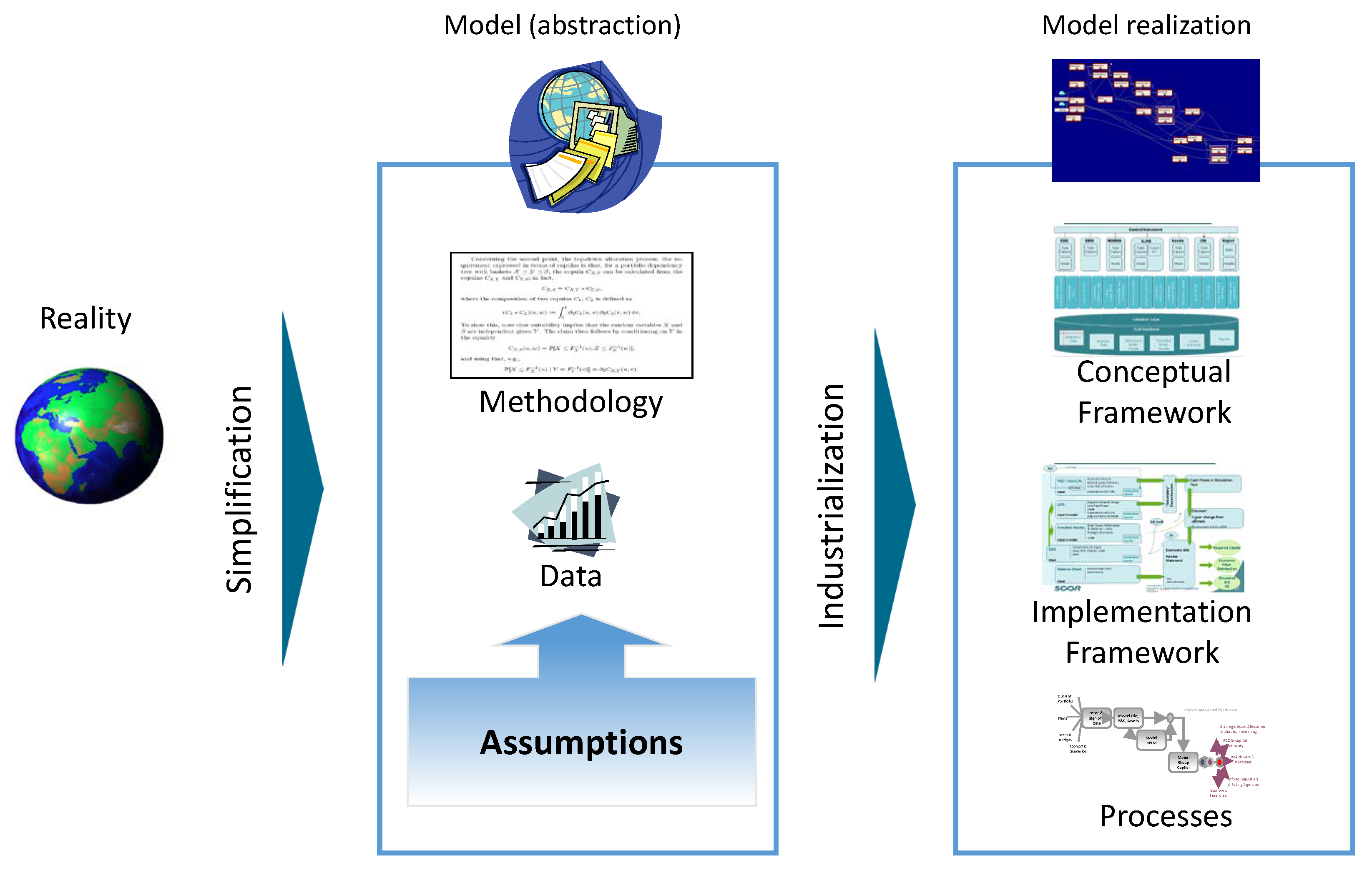
Figure 1.
Schematic representation of the modeling framework (Source: M. Dacorogna course on quantitative risk management, inspired by P. Keller).
Figure 1.
Schematic representation of the modeling framework (Source: M. Dacorogna course on quantitative risk management, inspired by P. Keller).

In Figure 1, we schematically illustrate the points we present in this section starting from the reality to be modeled to the industrialization phase that is needed to ensure a smooth production of risk results. All these components are mentioned in the three appendices but are not structured in the same way. Model validation will, of course, need to be designed around the structure described in Figure 1 and around the various points mentioned above. The final validation report will then be much more understandable and could be reused for future validations, as regular validation is a pre-requisite of the regulators.
In the banking sector, a very important procedure is backtesting, where VaR computations are tested against historical realizations (Christoffersen and Pelletier 2004). There is a vast literature on this subject (for a review, see, for instance Campbell (2005)). Recently, methods have also been developed for expected shortfall (see Acerbi and Szekely (2014); Kratz et al. (2018) and the references therein). However, this is not relevant here, as it applies to risk measures calculated over daily or bi-weekly data while, in the insurance case, we are talking about yearly time horizons and threshold at 99.5%, which means a 1-in-200-year event. In some particular cases, as we shall see in Section 3.2.1, we introduce another form of backtesting, the probability integral transform (Diebold et al. 1998), for checking the validity of economic scenario generators.
Having a clear understanding of what needs to be done provides a good framework to organize the validation process around these points. Let us now present a few validation procedures.
3. Model Implementation and Testing
In this section, we study the various ways to test the validity of the model based on the implementation of these models.
3.1. Calibration
The first step in a good validation procedure is to make sure that the calibration of model parameters is done properly. These parameters are set by fitting them to the data of the underlying process. Pricing and reserving actuaries often develop their models based on statistical tests on claims data. This is called “experience rating”. Sometimes, they also use risk models based on exposure data, for instance in modeling natural catastrophes (“exposure rating”). There are many models to estimate the one-year variability of claims reserves (see, for instance, Ferriero (2016) or Wüthrich and Merz (2008)). In general, internal models are usually composed of probabilistic models for the various risk drivers, but can also be composed of specific models for the dependence between those risks. Both sets of models need to be calibrated. The most difficult part is to find the right dependencies between risks because this requires lots of data. The data requirement is even more difficult to achieve when there are dependencies in the tails only. As mentioned above, the probabilistic models are usually calibrated with claims data for the liabilities and with market data for the assets. In other cases, such as for natural catastrophes, pandemics, or credit risk, stochastic models are used to produce probability distributions based on Monte Carlo simulations.
The new and difficult part of the calibration is the estimation of the dependencies between risks. This step is indispensable for the accurate aggregation of various risks. Dependencies cannot be adequately described by one number such as a linear correlation coefficient (as is often done even with big data analytics). Nevertheless, linear correlation is the most used dependence model in our industry. Most reinsurers, however, have long used copulas to model non-linear dependence. However, there is often not enough liability data to estimate the copulas. Experts usually have reliable opinions about conditional probabilities in the portfolio. These can be used to calibrate the copulas between the risks Arbenz and Canestraro (2012). The first step is to select a copula with an appropriate shape, usually with increased dependencies in the tail. This feature is observable in certain insurance data but is also known from stress scenarios. Then, one tries to estimate conditional probabilities by asking questions such as, “What about risk Y if risk X turned very bad?” To answer such questions, one needs to think about adverse scenarios in the portfolio or to look for causal relations between risks.
An internal model usually contains many risks. For instance, SCOR’s1 model contains a few thousand risks, which means a large amount of parameters to describe the dependence within the portfolio. The strategy for reducing the number of parameters must start from the knowledge of the underlying business. This allows us to concentrate our efforts on the main risks and to neglect those that are, by their nature, less dependent. One way of doing this is to develop a hierarchical model for dependencies, where models are aggregated first and then aggregated on another level with a different dependence model. This would reduce the parameter space and concentrate efforts on describing more accurately the main sources of dependent behavior. A hierarchical tree is defined by its topology while the number of parameters to estimate is reduced from essentially to n, where n is the number of risks included in the model. One of course pays a price for this reduction in terms of having to introduce assumptions about the risks for this structure to be a valid way to model their dependencies. If the upper level is modeled by a random variable (rv) Z and the lowest level by a rv X, the condition for using a hierarchical tree is:
In other words, given that the result of Y influences the information about the result in Z, the latter is not influenced by the distribution of X in Y. Given this assumption, the deeper the tree, the lower the dependence between risks at the lowest level. At the limit, in the case of a Gaussian tree (dependencies modeled with Gaussian copula), one can show that the dependence at the lowest level tends to zero when the depth of the tree tends to infinity. Business knowledge helps to separate the various lines of business to build such a tree with its different nodes (see Bruneton (2011) for a discussion of the Gaussian case).
Once the structure of dependence for each node is determined, there are two possibilities:
- If a causal dependence is known, it should be modeled explicitly.
- Otherwise, if there is no specific knowledge, non-symmetric copulas (e.g., Clayton copula) should be systematically used in the presence of a tail dependence for large claims.
To calibrate the various nodes, we again have two possibilities:
- If there are enough data, we calibrate the parameters statistically.
- In absence of data, we use stress scenarios and expert opinion to estimate conditional probabilities.
For the purpose of eliciting expert opinion (on common risk drivers, conditional probabilities, bucketing to build the tree, etc.), Arbenz and Canestraro have developed a Bayesian method combining various sources of information in the estimation: PrObEx (Arbenz and Canestraro 2012). This is a new methodology developed to ensure the prudent calibration of dependencies within and between different insurance risks. It is based on a Bayesian model that enables up to three sources of information to be combined:
- Prior information (i.e., indications from regulators or previous studies);
- Observations (i.e., the available data);
- Experts’ opinions (i.e., the knowledge of the experts).
For the last source, experts are invited to a workshop where they are asked to assess dependencies within their lines of business. The advantage of an approach using copulas is that they can be calibrated once a conditional probability is known. The latter are much easier to assess by experts than a correlation parameter. Once the elicitation process is completed, the database of answers can also be assessed for biases. If our business experience is that there is dependence between large claims, lack of data cannot be an excuse to use the wrong model. This lack of data can be compensated by a rigorous process of integrating expert opinions in the calibration.
3.2. Component Testing
Every internal model contains important components that will condition the results. Here is a generic list of main components for a (re)insurer:
- An economic scenario generator, to explore the various states of the world economy;
- A stochastic model to compute the uncertainty of P&C reserving triangles;
- A stochastic model for natural catastrophes;
- A stochastic model for pandemics (if there is a significant life book);
- A model for credit risk;
- A model for operational risk; and
- A model for risk aggregation.
Each of these components can be tested independently, to check the validity of the methods employed. These tests vary from one component to the other. Each requires its own approach for testing. We briefly describe below some of the approaches that can be used for testing some components.
3.2.1. Testing Economic Scenario Generators with Probability Integral Transform
We start with the economic scenario generator (see Müller et al. (2004)), as it is a component that can be tested against market data and is central to the valuation of both assets and liabilities. The economic scenario generator produces many scenarios, i.e., many different “forecast” values. Thousands of scenarios together define forecast distributions. We use backtesting to check how well realized variable values fit the prior forecast distribution for this variable. Here, we need to test the validity of the forecast of a distribution, which is less straightforward than testing point forecasts. The testing method we chose is the probability integral transform (PIT) advocated in Diebold et al. (1998) and Diebold et al. (1999). The objective is to determine the cumulative probability of a real variable value given its prior forecast distribution. The main idea of the method is to test the probability of each realized value in the distribution forecast.
Following is a summary of the steps (Müller et al. (2004)):
- We define an in-sample period to build the economic scenario generator with its innovation vectors and parameter calibrations (e.g., for the GARCH model). The out-of-sample period starts at the end of the in-sample period. Starting at each regular out-of-sample time point, we run a large number of simulation scenarios and observe the scenario forecasts for each of the many variables of the model (see Blum (2005)).
- The scenario forecasts of a variable x at time , sorted in ascending order, constitute an empirical cumulative distribution forecast. Considering many scenarios, this distribution converges asymptotically (with respect to the number of scenarios) to the marginal cumulative probability distribution , where is the information available up to the time of the simulation start. In the case of a one-step-ahead forecast, . The empirical distribution slightly deviates from . The discrepancy can be quantified (Blum 2005). For instance, its absolute value is less than 0.019 with a confidence of 95% when choosing 5000 scenarios for any value of x and any tested variable. This is accurate enough, given the limitations due to the rather low number of historical observations.
- For a set of out-of-sample time points , we now have a distribution forecast as well as a historically observed value . The cumulative distribution is used for the following probability integral transform (PIT): ). The probabilities , which are confined between 0 and 1 by definition, are used in the further course of the test. A proposition proved by Diebold et al. (1998) states that the are i.i.d. (independent and identically distributed) with a uniform distribution if the conditional distribution forecast coincides with the true process by which the historical data have been generated. The proof is extended to the multivariate case in Diebold et al. (1999). If the series of significantly deviates from either the distribution or the i.i.d. property, the model does not pass the out-of-sample test.
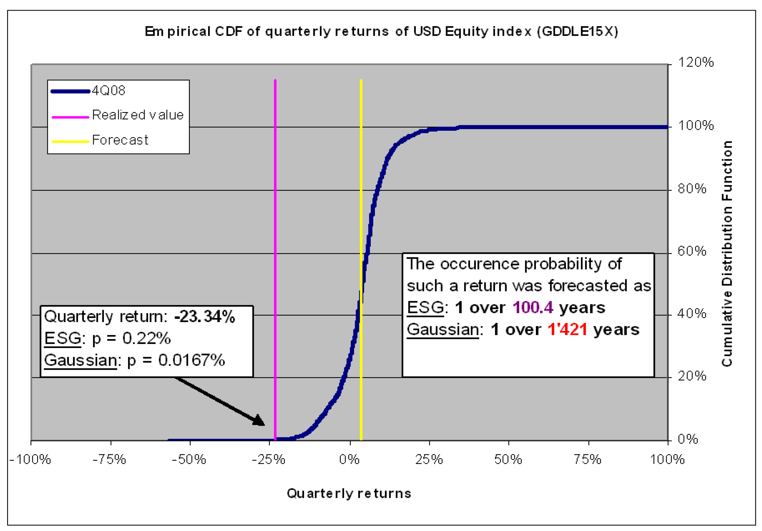
In Figure 2, we illustrate the PIT procedure on an example. We display the forecast of the cumulative distribution of returns of a U.S. stock index as produced in June 2007 for the fourth quarter of 2018. We also draw the expected value (yellow vertical line) and the value actually reached at that time (−23.34%, purple vertical line) and look at its probability in our forecast. We note that our model had, in June 2007, a much too optimistic expectation for the fourth quarter of 2008. We remind the reader that the economic scenario generator is not designed to be a point forecast model but to assess the risk of a particular financial asset. We see that it does this pretty well; in June 2007, it attributed a reasonable probability (1 in 100 years) to the occurrence of the fourth quarter of 20082, while the Gaussian model gave an extremely low probability of less than 1 in 1400 years. This is an extreme case, but it shows how the PIT test can be applied to all the important outputs of the economic scenario generator to check its ability to predict a good distribution, and thus the risk, of various economic variables.
3.2.2. Testing the One-Year Change of P&C Reserves
One of the biggest changes in the methodology that has been initiated by the new risk-based regulation is the computation of the one-year risk of P&C reserves. It is an important component of any P&C insurance risk. Testing the quality of the model to compute the one-year change is thus also one of the important steps towards validating a model. There are many ways one can think of testing this. We present here a method developed recently (see Dacorogna et al. (2018a)) that can also be applied for other validation procedures. It consists of designing simple stochastic models to reach the ultimate claim value that can then be used to simulate sample paths to test the various methods for computing the one-year change risk. Since claims data are too scarce to carry out rigorous statistical tests on the methods, with these models, we generate enough data to apply the methods. The advantage of this approach is that, by choosing simple models, one is able to obtain analytic or semi-analytic solutions for the risk against which the statistical methods can be tested.
In this example, we present the results of the model testing using two methods to compute the one-year change risk:
- The approach proposed by Wüthrich and Merz (2008) as an extension of the chain-ladder following Mack’s assumptions (Mack 1993). They obtain an estimation of the mean square error of the one-year change based on the development of the reserve triangles using the chain-ladder method.
- An alternative way to model the one-year risk, developed by Ferriero, is the capital over time (COT) method (Ferriero 2016). The latter assumes a modified jump-diffusion Lévy process to the ultimate risk and provides a formula, based on this process, to determine the one-year risk as a portion of the ultimate risk.
Here we present results, obtained in Dacorogna et al. (2018a), for two simple stochastic processes to reach the ultimate risk and for which we have derived explicit formulae:
- a model where the stochastic errors propagate linearly (linear model);
- a model where the stochastic errors propagate multiplicatively (multiplicative model).
For both processes, we compare the two methods mentioned above to see how they perform in assessing a risk that we explicitly know thanks to the analytic solutions of our models. The linear model does not follow the assumptions under which the chain-ladder model works. We thus expect that the Merz–Wüthrich method will perform poorly.
In Table 1, we present capital results for the linear model. The mean is the one-year capital, while the reserves are 101.87 with the chosen parameters. This is the typical capital intensity (capital over reserves) of the standard formula of Solvency II (15% to 20%). We immediately see that the Merz–Wüthrich method gives results that are way off due to the fact that its assumptions are not fulfilled. This illustrates the fact that the choice of an appropriate method is crucial for obtaining credible results. We also see that the COT method gives more reasonable numbers both with and without jumps.
The multiplicative model is better suited for the chain-ladder assumptions as we can see in Table 1, where we report similar results for the Merz–Wüthrich model. As is to be expected, the capital intensity is higher than for the linear model (29%), as multiplicative fluctuations are stronger than linear ones. In this case, all the methods underestimate the capital, but all of them perform similarly. The standard deviation is smallest for Merz–Wüthrich, but the error is the largest. One should also note here that the COT with jumps provides the best results, as one would expect due to the nature of the stochastic process, which involve large movements.
This example is presented here to illustrate the fact that one can, with such an approach, test the use of certain methods and gain confidence about their ability to deliver credible results for the risk3. In general, a technique to compensate for the lack of data is to design models that can generate data where the result is known and use this data to test the methods. It is what we also do in the next section.
3.2.3. Testing the Convergence of Monte Carlo Simulations
One of the most difficult and least-tested quantities is the number of simulations used to obtain aggregated distributions. Until recently, internal models would use 10,000 simulations. Nowadays, 100,000 simulations seem to have become the benchmark without clear justifications other than the capacity of the computers and the quality of the software. Nevertheless, it is important to know how well the model converges. The convergence of the algorithm is definitely an important issue when one is aggregating a few hundred or thousand risks with their dependencies. One way to do this is to obtain analytical expressions for the aggregated distribution and then test the Monte Carlo simulation against this benchmark.
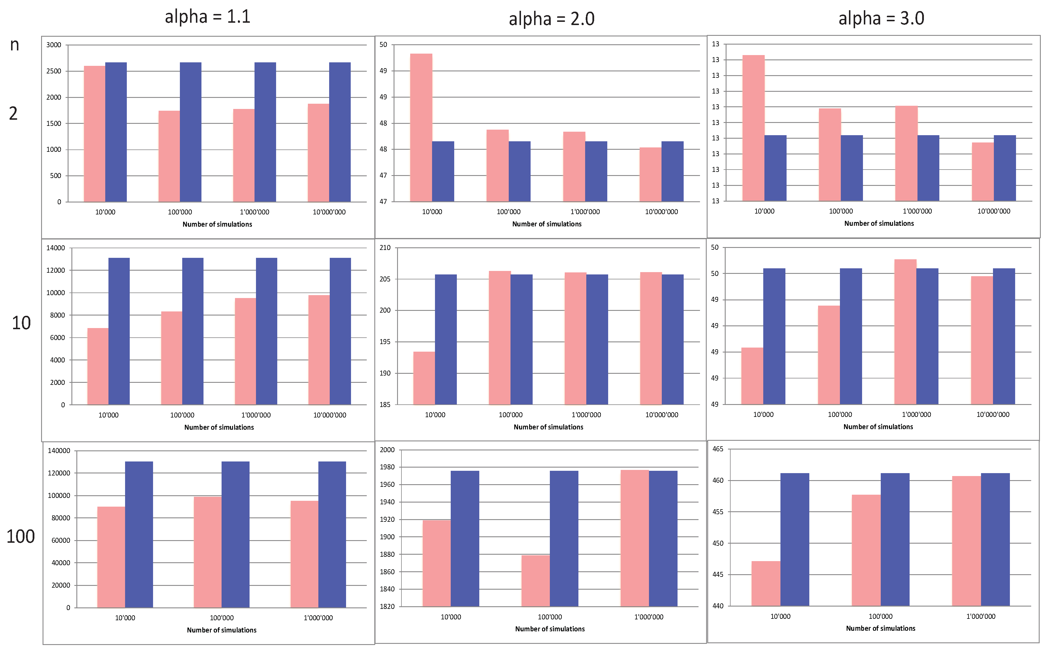
This is the path explored in Dacorogna et al. (2018b), where we give explicit formulae for the aggregation of Pareto distributions coupled with Clayton survival copulae and Weibull distributions coupled with Gumbel copulae. In Figure 3, we present results for the normalized TVaR (expected shortfall) () for various tail indices and different levels of aggregation . In the figure, we can see that, for a TVaR computed at a threshold and for a Clayton parameter :
- The normalized TVAR of , , decreases as n increases;
- The TVaR decreases as increases;
- The rate of convergence of increases with n;
- The heavier the tail (i.e., the lower the ), the slower the convergence;
- In the case of a very heavy tail and a strong dependence ( and ), we do not see any satisfactory convergence, even with 10 million simulations and for any n;
- When , the convergence is good from 1 million, 100,000 simulations onwards, respectively.
The advantage of having explicit expressions for the aggregation becomes evident here: We can explore in detail the convergence of the Monte Carlo (MC) simulations.
We can go one step further by looking at other quantities of interest. For this, we also define the diversification benefit as in Bürgi et al. (2008). Recall that the diversification performance of a portfolio is measured on the gain of capital when considering a portfolio of risks instead of a sum of the capital for the standalone risks. The capital is defined by the deviation from the expectation, and the diversification benefit (see Bürgi et al. (2008)) at a threshold (), by
where denotes a risk measure at threshold . This indicator helps to determine the optimal portfolio of the company since diversification reduces the risk and thus enhances the performance. By making sure that the diversification benefit is maximal, the company obtains the best performance for the lowest risk. However, it is important to note here that is not a universal measure and depends on the number of risks undertaken and the chosen risk measure.
The convergence appears even more clearly in the following Table 2.
In Table 2, we can see a decreasing estimation error by MC when increasing the aggregation factor, with small errors for and 2 and substantial errors for very fat tails and strong dependence. In the latter, we also see a systematic underestimation of the TVaR and an overestimation of the diversification benefit, whatever the aggregation factor. With thinner tails and lower dependence, MC has a tendency to overestimate the TVaR and underestimate the diversification benefit, except for ; note that the error decrease is large between 2 and 10 but much smaller afterwards4.
Overall, we see that, if , the convergence is good with 100,000 simulations. Problems start when . Luckily, the first case is the most common case for (re)insurance liabilities, except for earthquakes, windstorms, and pandemics. This is reassuring, even though it is not clear what would happen with small s and very strong dependence. More work along these lines is still needed to fully understand the convergence of MC given various parameters for the tails and the dependencies.
3.3. Stress Test to Validate the Distribution
Stress testing the model means that one has to look at the way the model reacts to a change of inputs. There are at least three ways of stress testing a model:
- Testing the sensitivity of the results to certain parameters (sensitivity analysis);
- Testing the predictions against real outcomes (historical test, via P&L attribution for lines of business (LoB) and assets);
- Testing the model outcomes against predefined scenarios.
The sensitivity analysis is important. It is not possible to base management decisions on results that could drastically change if some unimportant parameters are modified in the input. Unfortunately, note that this statement contains the adjective “unimportant”, which is hard to define. Clearly, the question is delicate because one has to determine, in advance, what the parameters are to which the results are most sensitive. For instance, the results might be sensitive to the heaviness of the tails or the strength and the shape of the dependence. We studied one of these important parameters in the previous section on the convergence of the MC. An increase in the number of simulations should not affect the results too much. In any case, a sensitivity analysis must be conducted on all parameters, and the results should be discussed according to the expected effects these parameters should have. In certain cases, big variations in capital in particular should be expected when we change the assumptions that directly affect the risk.
The second point is closely related to the PIT method described in Section 3.2.1, except that here we do not have enough data to test if the probabilities are really i.i.d. The only thing we can do is ensure that the probabilities obtained are reasonable both at a disaggregated level (lines of business or types of assets) as well as at an aggregated level (company’s results for the whole business or for a large portfolio). This type of backtest must be performed each year, and with experience accumulating, we should be able to draw conclusions on the overall quality of the forecast. In a way, we are testing here the belly of the distribution rather than the tails; nevertheless, this is also important as day-to-day decisions often have to do with those types of probability in mind rather than the extremes.
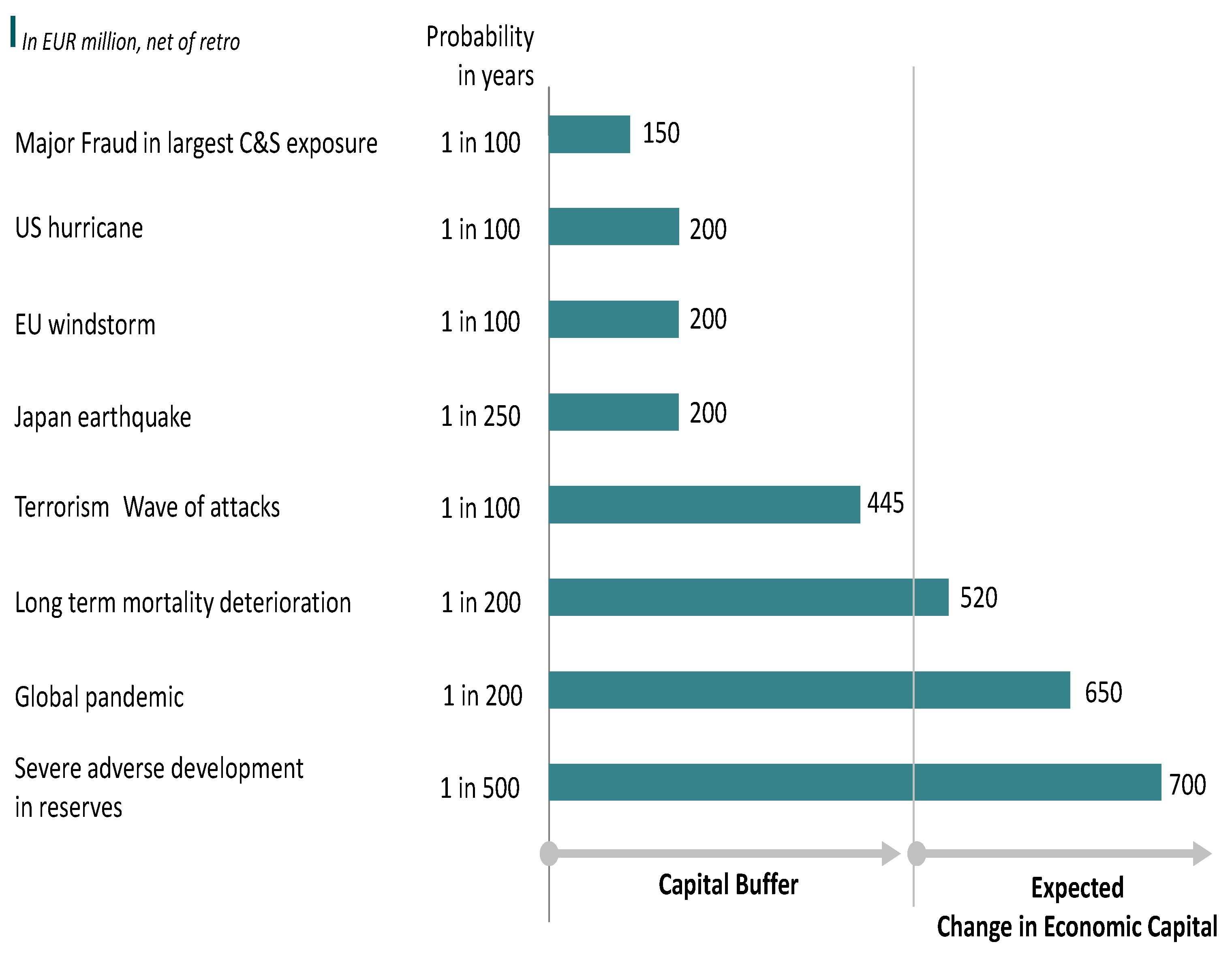
Scenarios can be seen as thought experiments about possible future states of the world. Scenarios are different from sensitivity analyses where the impact of a (small) change to a single variable is evaluated. Scenario results can be compared to simulation results in order to assess the probability of the scenarios in question. By comparing the probability of the scenario given by the internal model to the expected frequency of such a scenario, we can assess whether the internal model is realistic and has actually taken into account enough dependencies between risks. Recently, scenarios have caught the interest of regulators because they enable both management and regulators to visualize and understand plausible events. On the one hand, analyzing the impact on the company of a big natural catastrophe or a serious financial crisis is a good way to gain confidence in the value of the risk assessment made by the quantitative models. On the other hand, using only scenarios to estimate the capital needed for the company is a guarantee that the next crisis, which is bound to come from an unseen combination of events, will not be included in the model. That is why a combination of probabilistic approaches and scenarios is a good way of validating model results. In Figure 4, we present an example published by SCOR some years ago showing the impact of some scenarios on the balance sheet of the company measured against the capital buffer the company holds for covering the risks.
3.4. Using Monte Carlo Simulations to Validate Dependence Assumptions
Internal models based on stochastic Monte Carlo simulations produce many scenarios at each run (typically a few thousand). Usually very little of these data are used: some averages for computing capital as well as some expectations. However, these outputs can be put to use for understanding the way the model works. One example could be to select the worst cases and look at the scenarios that make the company bankrupt. Two questions to ask about these scenarios:
- Are these scenarios credible, given the company portfolio? Would such scenarios really affect the company?
- Are there other possible scenarios that we know of and that do not appear in the worst Monte Carlo simulations?
If the answers to the first question is positive and negative to the second, we gain confidence in the way the model reflects the extreme risks and describes our business. Inversely, one could consider how often the model would give negative results after one year. If this probability is very low, we would know that our model is too optimistic and would probably underestimate the extreme risk. If the answer is the opposite, the conclusion would be that our model is too conservative and neglects some of our business realities. In the case of reinsurance, looking at the published balance sheets, a typical frequency of negative results would be once every ten years for a healthy reinsurance company. This is the kind of reverse backtesting that can be done on simulations to explore the quality of the results.
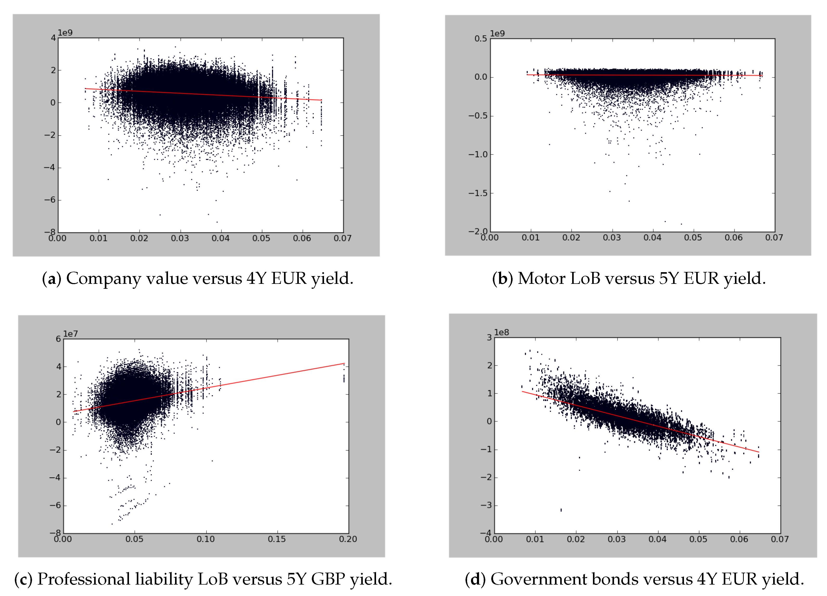
Other tests, such as looking at conditional statistics, can be envisaged and are also interesting. A typical question would be, for instance, how is the capital going to behave if interest rates rise? Exploring the dependence of results on certain important variables is a very good way to test the reasonableness of the dependence model. As we already explained, validation of internal models does not mean statistical validation because there will never be enough data to reach a good conclusion at high enough significance levels. In this context, reasonableness, given our knowledge of the business and past experience, is the most we can hope to achieve. In Figure 5, we present regression plots where we show the dependency between interest rates and changes in economic value (of the overall company portfolio and for several sub-portfolios). The plots are based on the full 100,000 scenarios of the Monte Carlo simlations. By analyzing the internal model results at this level, we can follow up on a lot of effects and test if they make sense.
We start this example with the change in economic value of the company after one year that is displayed in Figure 5a. We choose to do a regression against the 4Y EUR government yield because the liability portfolio of this company has a duration of roughly 4Y and the balance sheet is denominated in EUR. In all the graphs, the chosen interest rate is the one corresponding to the currency denomination of the portfolio and its duration. We see that the value of the company is slightly lower in the scenarios where interest rates rise. This decrease is due to an increase in inflation, which is linked to an increase of interest rates in our economic scenario generator. This slight dependence on interest rate would not happen if the asset and liability management (ALM) of the company was perfect. Therefore, this is also an indirect way to test the efficiency of the ALM policy. However, in this case, we understand the behavior shown in this reverse stress test since, by fear of inflation, the company had invested a good portion of its assets in inflation-linked bonds that have a non-linear reaction to interest rate movements.
In Figure 5b, we regress the change in economic value of motor LoB versus the 5Y EUR yield. The value of motor business depends only very weakly on interest rate as it is a relatively short tail. This is reflected here in the figure through the regression line that is parallel to the x-axis. In Figure 5c, we show the regression between the change in economic value of professional liability and the 5Y GBP yield. The value of professional liability business depends heavily on interest rate, as it takes a long time to develop to ultimate risk, and the reserve can earn interest for a longer time. Indeed, the regression line reflects this very well. The last graph displayed in Figure 5d is related to the regression of the change in economic value of the government bond asset portfolio and the 4Y EUR yield. Here the relation is obvious and also well-reflected in the simulations: bond values depend mechanically on interest rates. When interest rates increase, the value decreases. The dispersion we see on the graph is simply due to the fact that not all bonds have a duration of 4Y.
Looking at all these graphs helps to convince ourselves that the behavior of the various risks captured in the portfolio with respect to interest rates is well-described by the model and that dependence on this very important risk driver for the insurance business is well-modeled. It is another means of gaining confidence in the accuracy of the model, and it makes full use of the simulation results and not only some sort of average or one particular point on the probability distribution (like VaR, for instance). On these graphs, we can also inspect the dispersion around the regression line; it represents the uncertainty around the main behavior. For instance, we notice that, as expected, in Figure 5b,d, there is little dispersion, while in Figure 5a,c, we have a higher dispersion as the interest rate is, by far, not the only risk driver of those portfolios. This is only an example of the many dimensions that can be validated this way. It is definitely an important piece of our toolbox for gaining confidence in the results of our models.
4. Conclusions
The development of risk models is an important step to improve risk awareness in the company and anchor risk management and governance deeper in industry practices. With risk models, quantitative analysts provide management with valuable risk assessments, especially in relative terms, as well as guidance in business decisions. Quantitative assessment of risk helps to place the discussion on a sensible level rather than being based on unfounded arguments. It is thus essential to ensure that the results of the model provide a good description of reality. In this paper, we have not presented numerical results of the risk assessment because, apart from the solvency ratio and risk-adjusted capital, companies do not disclose intermediate values and, as already explained, it is not possible to test the capital values directly. The purpose of this paper is to present strategies for testing the model. However, it should be understood that RIMs require a significant amount of time to run. In our case, the model took a few hours to run on powerful machines. This makes it all the more important to have indirect methods to test the validity of the results.
Model validation is the way to gain confidence in the model and ensure its acceptance by all stakeholders. However, this is a difficult task because there is no straightforward way of testing the many outputs of a model. As illustrated in this paper, it is only by combining various approaches that we can come to a conclusion regarding the suitability of the risk assessment.
Among the strategies to validate a model, let us recall those that we presented or mentioned in this paper:
- Ensure a good calibration of the model through various statistical techniques;
- Use data to statistically test certain parts of the model (like the computation of the risk measure, or some particular model like economic scenario generator or reserving risk);
- Test the P&L attribution to LoBs against real outcomes;
- Test the sensitivity of the model to crucial parameters;
- Compare the model output to stress scenarios;
- Compare the real outcome to the probability predicted by the model;
- Examine the simulation output to check the quality of the bankruptcy scenarios.
Beyond pure statistical techniques, this list provides a useful set of methods to obtain a better understanding of the model behavior and to convince management and regulators that the techniques used to quantify the risks are adequate and that the results really represent the risks facing the company. With the experience we are gaining, we will undoubtedly make progress in this field. We will also make further progress in the near future by doing research to define good strategies to test our models. As long as we keep in mind that we need to be rigorous in our approach and use the scientific method to assess the results, we will be able to improve both our models and their validation.
Funding
This research received no external funding.
Conflicts of Interest
The author declares no conflict of interest.
Appendix A. Article 124 on “Validation Standards” of the European Directive
Article 124
Validation Standards
Insurance and reinsurance undertakings shall have a regular cycle of model validation which includes monitoring the performance of the internal model, reviewing the ongoing appropriateness of its specification, and testing its results against experience.
The model validation process shall include an effective statistical process for validating the internal model which enables the insurance and reinsurance undertakings to demonstrate to their supervisory authorities that the resulting capital requirements are appropriate.
The statistical methods applied shall test the appropriateness of the probability distribution forecast compared not only to loss experience but also to all material new data and information relating thereto.
The model validation process shall include an analysis of the stability of the internal model and in particular the testing of the sensitivity of the results of the internal model to changes in key underlying assumptions. It shall also include an assessment of the accuracy, completeness and appropriateness of the data used by the internal model.
Appendix B. Article 241 on “Model Validation Process” of the Delegated Regulation of the 17th of January 2015
Article 241
Model Validation Process
- The model validation process shall apply to all parts of the internal model and shall cover all requirements set out in Articles 101, Article 112(5), Articles 120 to 123 and Article 125 of Directive 2009/138/EC. In the case of a partial internal model the validation process shall in addition cover the requirements set out in Article 113 of that Directive.
- In order to ensure independence of the model validation process from the development and operation of the internal model, the persons or organisational unit shall, when carrying out the model validation process, be free from influence from those responsible for the development and operation of the internal model. This assessment shall be in accordance with paragraph 4.
- For the purpose of the model validation process insurance and reinsurance undertakings shall specify all of the following:
- (a)
- the processes and methods used to validate the internal model and their purposes;
- (b)
- for each part of the internal model, the frequency of regular validations and the circumstances which trigger additional validation;
- (c)
- the persons who are responsible for each validation task;
- (d)
- the procedure to be followed in the event that the model validation process identifies problems with the reliability of the internal model and the decision-making process to address those problems.
Appendix C. Article 242 on “Validation Tools” of the Delegated Regulation of the 17th of January 2015
Article 242
Model Validation Tools
- Insurance and reinsurance undertakings shall test the results and the key assumptions of the internal model at least annually against experience and other appropriate data to the extent that data are reasonably available. These tests shall be applied at the level of single outputs as well as at the level of aggregated results. Insurance and reinsurance undertakings shall identify the reason for any significant divergence between assumptions and data and between results and data.
- As part of the testing of the internal model results against experience insurance and reinsurance undertakings shall compare the results of the profit and loss attribution referred to in Article 123 of Directive 2009/138/EC with the risks modeled in the internal model.
- The statistical process for validating the internal model, referred to in the second paragraph of Article 124 of Directive 2009/138/EC, shall be based on all of the following: (a) current information, taking into account, where it is relevant and appropriate, developments in actuarial techniques and the generally accepted market practice; (b) a detailed understanding of the economic and actuarial theory and the assumptions underlying the methods to calculate the probability distribution forecast of the internal model. 4. Where insurance or reinsurance undertakings observe in accordance with the fourth paragraph of Article 124 of Directive 2009/138/EC that changes in a key underlying assumption have a significant impact on the Solvency Capital Requirement, they shall be able to explain the reasons for this sensitivity and how the sensitivity is taken into account in their decision-making process. For the purposes of the fourth subparagraph of Article 124 of Directive 2009/138/EC the key assumptions shall include assumptions on future management actions.
- The model validation process shall include an analysis of the stability of the outputs of the internal model for different calculations of the internal model using the same input data.
- As part of the demonstration that the capital requirements resulting from the internal model are appropriate, insurance and reinsurance undertakings shall compare the coverage and the scope of the internal model. For this purpose, the statistical process for validating the internal model shall include a reverse stress test, identifying the most probable stresses that would threaten the viability of the insurance or reinsurance undertaking.
| 1 | SCOR is the fifth-largest reinsurance company with gross written premium of more than 19.7 billion EUR (10 billion for P&C and 9.7 billion for life and health in 2022). |
| 2 | The yearly return of 2008 was the second-worst performance of the S&P 500 measured over 200 years. Only the year 1933 presented a worse performance! |
| 3 | |
| 4 |
References
- Abramov, Vilen, and M. Kazim Khan. 2017. A Practical Guide to Market Risk Model Validations (Part II—VaR Estimation). SSRN 3080557. Available online: https://papers.ssrn.com/sol3/papers.cfm?abstract_id=2916853 (accessed on 4 May 2023).
- Abramov, Vilen, Matt Lowdermilk, and Xianwen Zhou. 2017. A Practical Guide to Market Risk Model Validations (Part I—Introduction). SSRN 2916853. Available online: https://papers.ssrn.com/sol3/papers.cfm?abstract_id=3080557 (accessed on 4 May 2023).
- Acerbi, Carlo, and Balazs Szekely. 2014. Back-testing expected shortfall. Risk 27: 76–81. [Google Scholar]
- Arbenz, Philipp, and Davide Canestraro. 2012. Estimating copulas for insurance from scarce observations, expert opinion and prior information: A bayesian approach. ASTIN Bulletin: The Journal of the IAA 42: 271–90. [Google Scholar]
- Bignozzi, Valeria, and Andreas Tsanakas. 2016. Parameter uncertainty and residual estimation risk. Journal of Risk and Insurance 83: 949–78. [Google Scholar] [CrossRef]
- Blum, Peter. 2005. On Some Mathematical Aspects of Dynamic Financial Analysis. Ph.D. thesis, ETH Zurich, Zürich, Switzerland. [Google Scholar]
- Bruneton, Jean-Philippe. 2011. Copula-based hierarchical aggregation of correlated risks. the behaviour of the diversification benefit in gaussian and lognormal trees. arXiv arXiv:1111.1113. [Google Scholar]
- Bürgi, Roland, Michel M. Dacorogna, and Roger Iles. 2008. Risk aggregation, dependence structure and diversification benefit. In Stress Testing for Financial Institutions. Edited by Daniel Rösch and Harald Scheule. London: Riskbooks, Incisive Media. [Google Scholar]
- Busse, Marc, Ulrich Müller, and Michel Dacorogna. 2010. Robust estimation of reserve risk. ASTIN Bulletin: The Journal of the IAA 40: 453–89. [Google Scholar]
- Campbell, Sean D. 2005. A Review of Backtesting and Backtesting Procedures. Finance and Economics Discussion Series (FEDS). Available online: https://www.federalreserve.gov/econres/feds/a-review-of-backtesting-and-backtesting-procedures.htm (accessed on 4 May 2023).
- Christoffersen, Peter. 1998. Evaluating interval forecasts. International Economic Review 39: 841–62. [Google Scholar] [CrossRef]
- Christoffersen, Peter, and Denis Pelletier. 2004. Backtesting value-at-risk: A duration-based approach. Journal of Financial Econometrics 2: 84–108. [Google Scholar] [CrossRef]
- Clemente, Gian Paolo, and Nino Savelli. 2013. Internal model techniques of premium and reserve risk for non-life insurers. Mathematical Methods in Economics and Finance 8: 21–34. [Google Scholar]
- Cox, David. 1995. Comment on “model uncertainty, data mining and statistical inference”. Journal of the Royal Statistical Society: Series A (Statistics in Society) 158: 455–56. [Google Scholar]
- Dacorogna, Michel, Alessandro Ferriero, and David Krief. 2018a. One-year change methodologies for fixed-sum insurance contracts. Risks 6: 75. [Google Scholar] [CrossRef]
- Dacorogna, Michel, Laila Elbahtouri, and Marie Kratz. 2018b. Validation of aggregated risks models. Annals of Actuarial Science 12: 433–54. [Google Scholar] [CrossRef]
- Dacorogna, Michel M., Ulrich A. Müller, Olivier V Pictet, and Casper G. De Vries. 2001. Extremal forex returns in extremely large data sets. Extremes 4: 105–27. [Google Scholar] [CrossRef]
- Diebold, Francis X., Todd A. Gunther, and Anthony S. Tay. 1998. Evaluating density forecasts with applications to financial risk management. International Economic Review 39: 863–83. [Google Scholar] [CrossRef]
- Diebold, Francis X., Jinyong Hahn, and Anthony S. Tay. 1999. Multivariate density forecast evaluation and calibration in financial risk management: High-frequency returns on foreign exchange. Review of Economics and Statistics 81: 661–73. [Google Scholar] [CrossRef]
- Dorofeev, Dmitriy, and Sergey Shestakov. 2018. 2-tier vs. 3-tier architectures for data processing software. Paper presented at the 3rd International Conference on Applications in Information Technology, Aizu-Wakamatsu, Japan, November 1–3; pp. 63–68. [Google Scholar]
- Embrechts, Paul. 2017. A darwinian view on internal models. Journal of Risk 20: 1–21. [Google Scholar] [CrossRef]
- Ferriero, Alessandro. 2016. Solvency capital estimation, reserving cycle and ultimate risk. Insurance: Mathematics and Economics 68: 162–68. [Google Scholar] [CrossRef]
- Fröhlich, Andreas, and Annegret Weng. 2015. Modelling parameter uncertainty for risk capital calculation. European Actuarial Journal 5: 79–112. [Google Scholar] [CrossRef]
- Fröhlich, Andreas, and Annegret Weng. 2018. Parameter uncertainty and reserve risk under Solvency II. Insurance: Mathematics and Economics 81: 130–41. [Google Scholar] [CrossRef]
- Grant, Stuart W., Gary S. Collins, and Samer A. M. Nashef. 2018. Statistical primer: Developing and validating a risk prediction model. European Journal of Cardio-Thoracic Surgery 54: 203–8. [Google Scholar] [CrossRef] [PubMed]
- Kratz, Marie, Yen H. Lok, and Alexander J. McNeil. 2018. Multinomial VaR backtests: A simple implicit approach to backtesting expected shortfall. Journal of Banking and Finance 88: 393–407. [Google Scholar] [CrossRef]
- Landry, Maurice, Jean-Louis Malouin, and Muhittin Oral. 1983. Model validation in operations research. European Journal of Operational Research 14: 207–20. [Google Scholar] [CrossRef]
- Lloyd’s. 2023. Internal Model Validation Guidance. Available online: https://www.lloyds.com/resources-and-services/capital-and-reserving/capital-guidance/model-validation/ (accessed on 1 April 2023).
- Mack, Thomas. 1993. Distribution-free calculation of the standard error of chain ladder reserve estimates. ASTIN Bulletin: The Journal of the IAA 23: 213–25. [Google Scholar] [CrossRef]
- Mc Neil, Alexander J., Rüdiger Frey, and Paul Embrechts. 2016. Quantitative Risk Management, 2nd ed. Princeton: Princeton Series in Finance. [Google Scholar]
- Meese, Richard A., and Kenneth Rogoff. 1983. Empirical exchange rate models of the seventies: Do they fit out of sample? Journal of International Economics 14: 3–24. [Google Scholar] [CrossRef]
- Miller, April R., Samin Charepoo, Erik Yan, Ryan W. Frost, Zachary J. Sturgeon, Grace Gibbon, Patrick N. Balius, Cedonia S. Thomas, Melanie A. Schmitt, Daniel A. Sass, and et al. 2022. Reliability of COVID-19 data: An evaluation and reflection. PLoS ONE 17: e0251470. [Google Scholar] [CrossRef]
- Morini, Massimo. 2011. Understanding and Managing Model Risk: A Practical Guide for Quants, Traders and Validators. New York: John Wiley & Sons. [Google Scholar]
- Müller, Ulrich A., Roland Bürgi, and Michel M. Dacorogna. 2004. Bootstrapping the Economy—A Non-Parametric Method of Generating Consistent Future Scenarios. Available online: https://ideas.repec.org/p/pra/mprapa/17755.html (accessed on 1 April 2023).
- Seitshiro, Modisane B., and Hopolang P. Mashele. 2020. Assessment of model risk due to the use of an inappropriate parameter estimator. Cogent Economics & Finance 8: 1710970. [Google Scholar] [CrossRef]
- Sornette, Didier, A. B. Davis, K. Ide, K. R. Vixie, V. Pisarenko, and J. R. Kamm. 2007. Algorithm for model validation: Theory and applications. Proceedings of the National Academy of Sciences of the United States of America 104: 6562–67. [Google Scholar] [CrossRef]
- Stricker, Markus, David Ingram, and Dave Simmons. 2013. Economic capital model validation. In White Paper, Willis Economic Capital Forum. London: Willis Limited. [Google Scholar]
- Wüthrich, Mario V., and Michael Merz. 2008. Stochastic Claims Reserving Methods in Insurance. New York: John Wiley & Sons. [Google Scholar]
- Zariņa, Ilze, Irina Voronova, and Gaida Pettere. 2019. Internal model for insurers: Possibilities and issues. Paper presented at the International Scientific Conference “Contemporary Issues in Business, Management and Economics Engineering”, Vilnius, Lithuania, May 9–10. [Google Scholar]
Figure 2.
Cumulative distribution forecast of a U.S. Equity Index made in June 2007 for 31 December 2008. The purple line is the actual realization, while the yellow line is the expectation of the distribution forecast (Source: M. Dacorogna course on quantitative risk management).
Figure 2.
Cumulative distribution forecast of a U.S. Equity Index made in June 2007 for 31 December 2008. The purple line is the actual realization, while the yellow line is the expectation of the distribution forecast (Source: M. Dacorogna course on quantitative risk management).

Figure 3.
Convergence of the TVaR of at 99.5% for from left to right, for an aggregation factor from top to bottom. The dark plots are for the analytical values, and the light ones are the average values obtained from the MC simulations. The y-scale gives the normalized TVaR () (source: Dacorogna et al. (2018b)).

Figure 4.
We display the results of scenarios that could affect the balance sheet of a reinsurance company with its estimated probability of occurence. We also compare the values to the size of the capital buffer and the expected next year profit of the company (source: SCOR investor’s day presentation 2008).

Figure 5.
We display here typical regression analyses on the simulation results of the internal model (source: M. Dacorogna course on quantitative risk management).
Figure 5.
We display here typical regression analyses on the simulation results of the internal model (source: M. Dacorogna course on quantitative risk management).


Table 1.
Statistics for the first-year capital on 500 simulated triangles with the linear model. The following are displayed: the mean first-year capital, the standard deviation of the capital around that mean, and the mean absolute and relative deviations (MAD, MRAD) from the true value. The mean value of reserves estimated with chain-ladder is 101.87, which is consistent with the reserves calculated with our model, i.e., (source: Dacorogna et al. (2018a)).
| Method | Mean | Std. Dev. | MAD | MRAD |
|---|---|---|---|---|
| Linear Model: | ||||
| Theoretical value | 18.37 | 3.92 | – | – |
| COT, without jumps | 19.08 | 3.93 | 0.71 | 4.14% |
| COT, with jumps | 18.81 | 3.86 | 0.43 | 2.47% |
| Merz–Wüthrich | 252.89 | 149.6 | 234.5 | 1365.6% |
| Multiplicative Model: | ||||
| Theoretical value | 29.36 | 21.97 | – | – |
| COT, without jumps | 26.75 | 19.84 | 2.54 | 8.19% |
| COT, with jumps | 28.30 | 20.98 | 1.07 | 3.48% |
| Merz–Wüthrich | 22.82 | 15.77 | 12.7 | 43.2% |
Table 2.
Relative errors (when comparing results obtained by MC and analytical ones) of the and the diversification benefit for , at 99.5% and for various , as a function of the aggregation factor n computed with 1 million simulations (source: Dacorogna et al. (2018b)).
Table 2.
Relative errors (when comparing results obtained by MC and analytical ones) of the and the diversification benefit for , at 99.5% and for various , as a function of the aggregation factor n computed with 1 million simulations (source: Dacorogna et al. (2018b)).
| n = 2 | n = 10 | n = 100 | |
|---|---|---|---|
| α = 3 | |||
| 0.30% | 0.14% | −0.10% | |
| −1.30% | −0.25% | 0.15% | |
| α = 2 | |||
| 0.38% | 0.14% | 0.05% | |
| −2.61% | −0.44% | −0.14% | |
| α = 1.1 | |||
| −33.3% | −27.3% | −26.9% | |
| 1786% | 742% | 653% |
Disclaimer/Publisher’s Note: The statements, opinions and data contained in all publications are solely those of the individual author(s) and contributor(s) and not of MDPI and/or the editor(s). MDPI and/or the editor(s) disclaim responsibility for any injury to people or property resulting from any ideas, methods, instructions or products referred to in the content. |
© 2023 by the author. Licensee MDPI, Basel, Switzerland. This article is an open access article distributed under the terms and conditions of the Creative Commons Attribution (CC BY) license (https://creativecommons.org/licenses/by/4.0/).
Share and Cite
MDPI and ACS Style
Dacorogna, M. How to Gain Confidence in the Results of Internal Risk Models? Approaches and Techniques for Validation. Risks 2023, 11, 98. https://doi.org/10.3390/risks11050098
AMA Style
Dacorogna M. How to Gain Confidence in the Results of Internal Risk Models? Approaches and Techniques for Validation. Risks. 2023; 11(5):98. https://doi.org/10.3390/risks11050098
Chicago/Turabian StyleDacorogna, Michel. 2023. "How to Gain Confidence in the Results of Internal Risk Models? Approaches and Techniques for Validation" Risks 11, no. 5: 98. https://doi.org/10.3390/risks11050098
Note that from the first issue of 2016, this journal uses article numbers instead of page numbers. See further details here.