
A Computer-Aided Diagnostic System to Identify Diabetic Retinopathy, Utilizing a Modified Compact Convolutional Transformer and Low-Resolution Images to Reduce Computation Time
 , , , , ,
Abstract
:1. Introduction
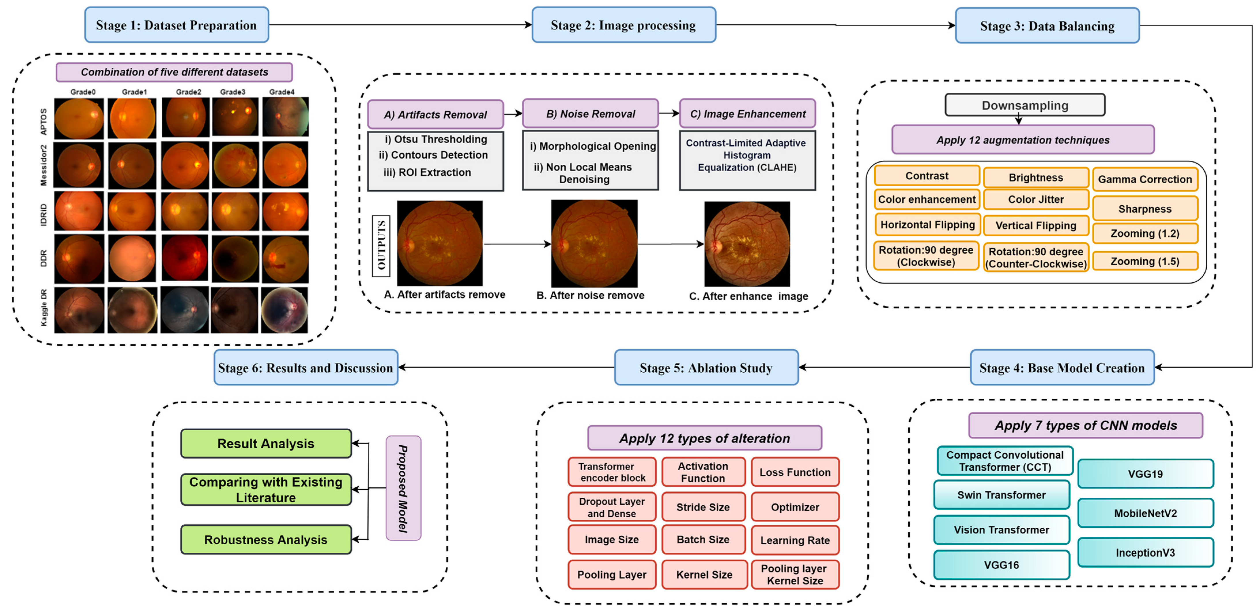
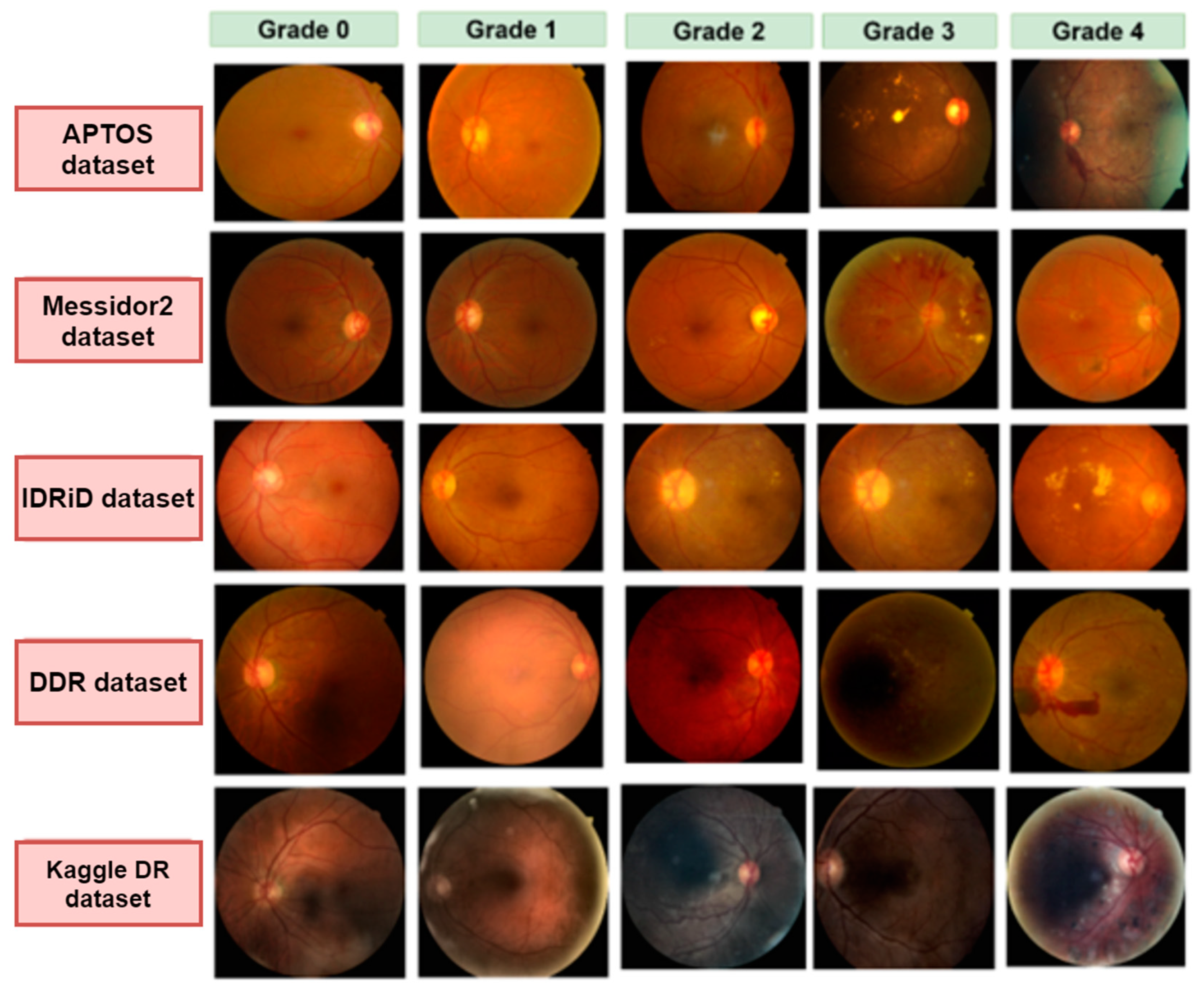
- A total of five datasets are amalgamated to generate a larger and more encompassing dataset, and a wide range of diabetic retinopathy images with diverse resolutions and image quality are utilized. The resulting datahub contains 53,185 raw images.
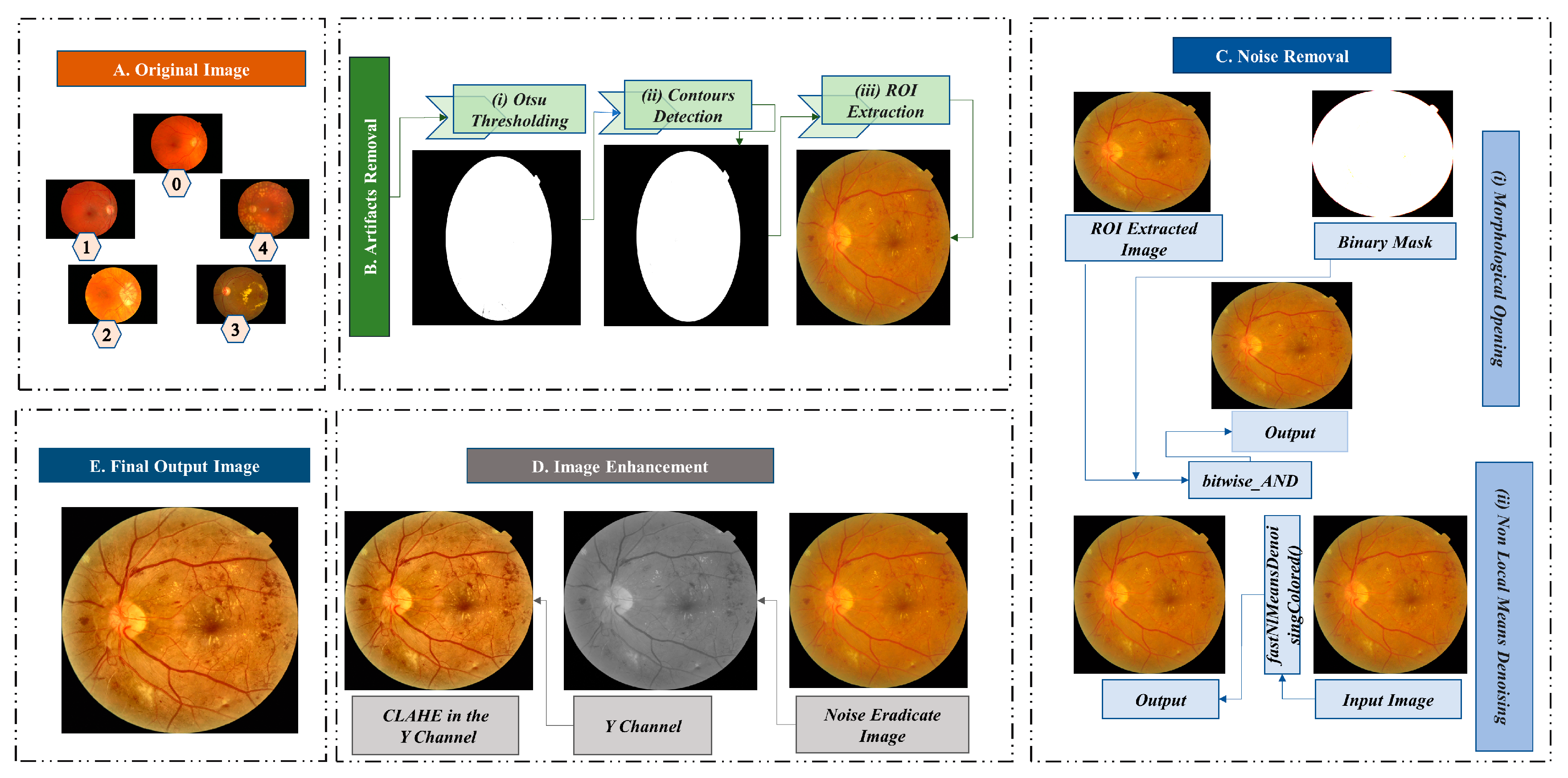
- Several image pre-processing techniques, including Otsu thresholding, contour detection, region of interest (ROI) extraction, morphological opening, non-local means denoising, and Contrast Limited Adaptive Histogram Equalization (CLAHE), are used to eliminate artifacts and noise from retinal fundus images and enhance their quality.
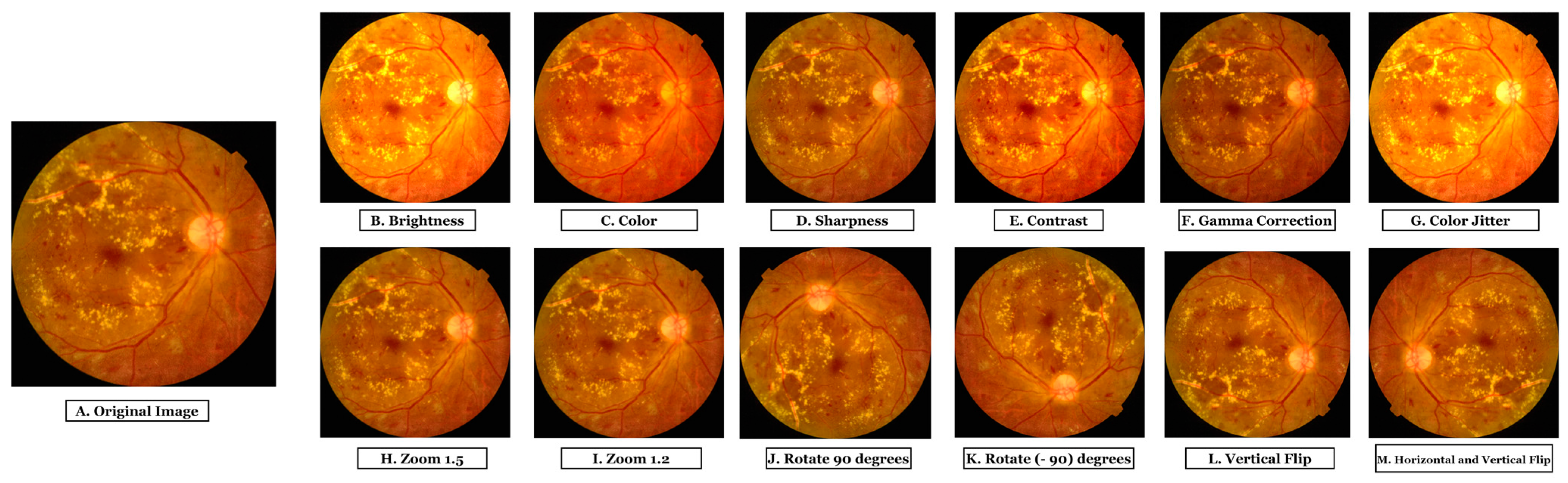
- An augmentation strategy is applied to increase the number of images and create a large data hub.
- A detailed comparison between three transformer models (Vision transformer, Swin transformer, and Compact Convolutional Transformer) and four transfer learning models (VGG19, VGG16, MobileNetV2, and ResNet50) using our dataset is done to evaluate how well the models perform in terms of accuracy and training time and to find the optimal transformer or transfer learning model for a vast number of images.
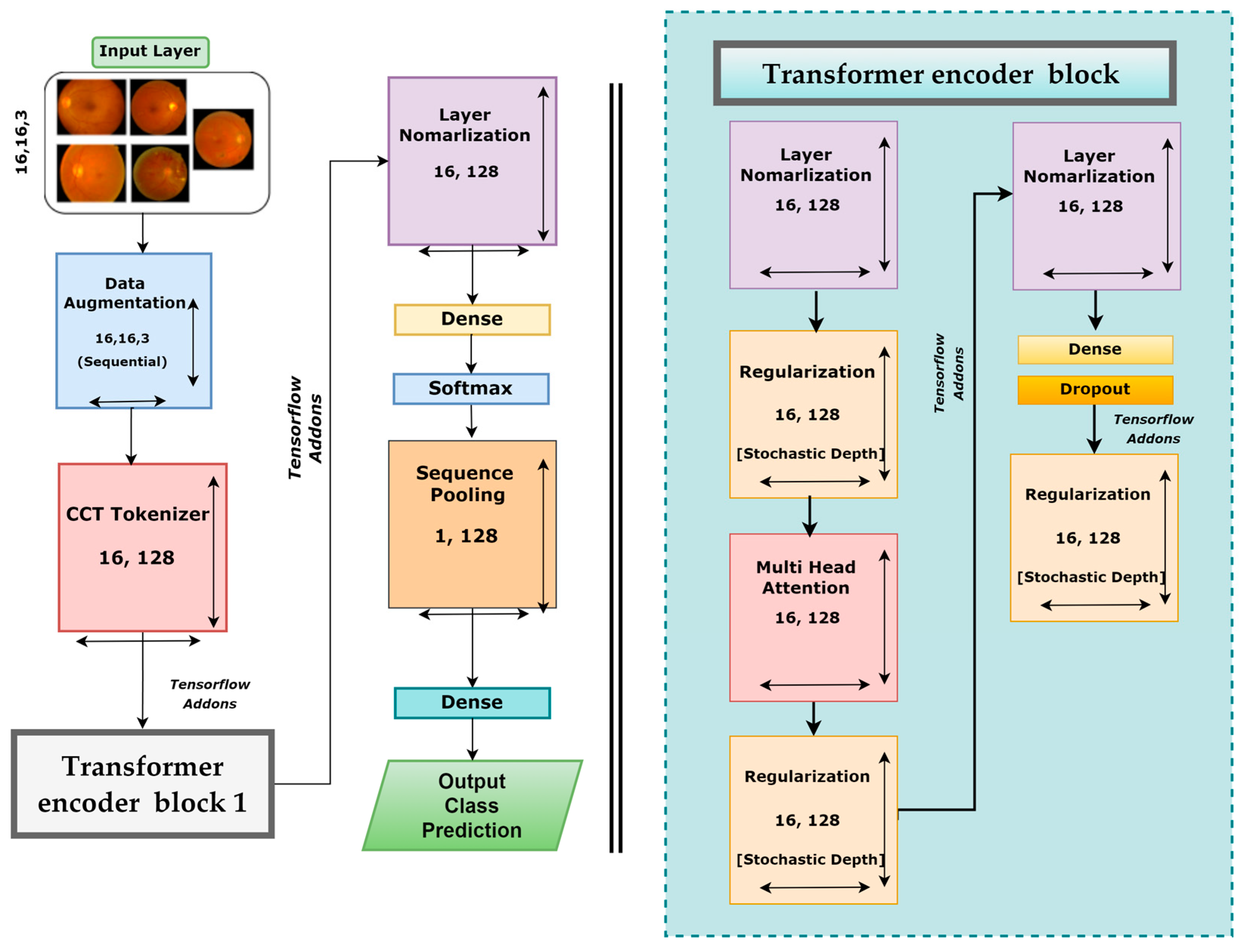
- A new model, DR-CCTNet, is proposed. It is constructed by modifying the original CCT model to overcome the long training times issue and work with a large data hub. Using convolutional blocks, the tokenization step of the vision transformer is accomplished, drastically lowering model training time while attaining high accuracy, even with low-pixel images.
- An ablation study is carried out by modifying the proposed model’s various hyper-parameters and layer architecture to improve its performance further, reducing the number of parameters and making the training process less complicated and time-consuming.
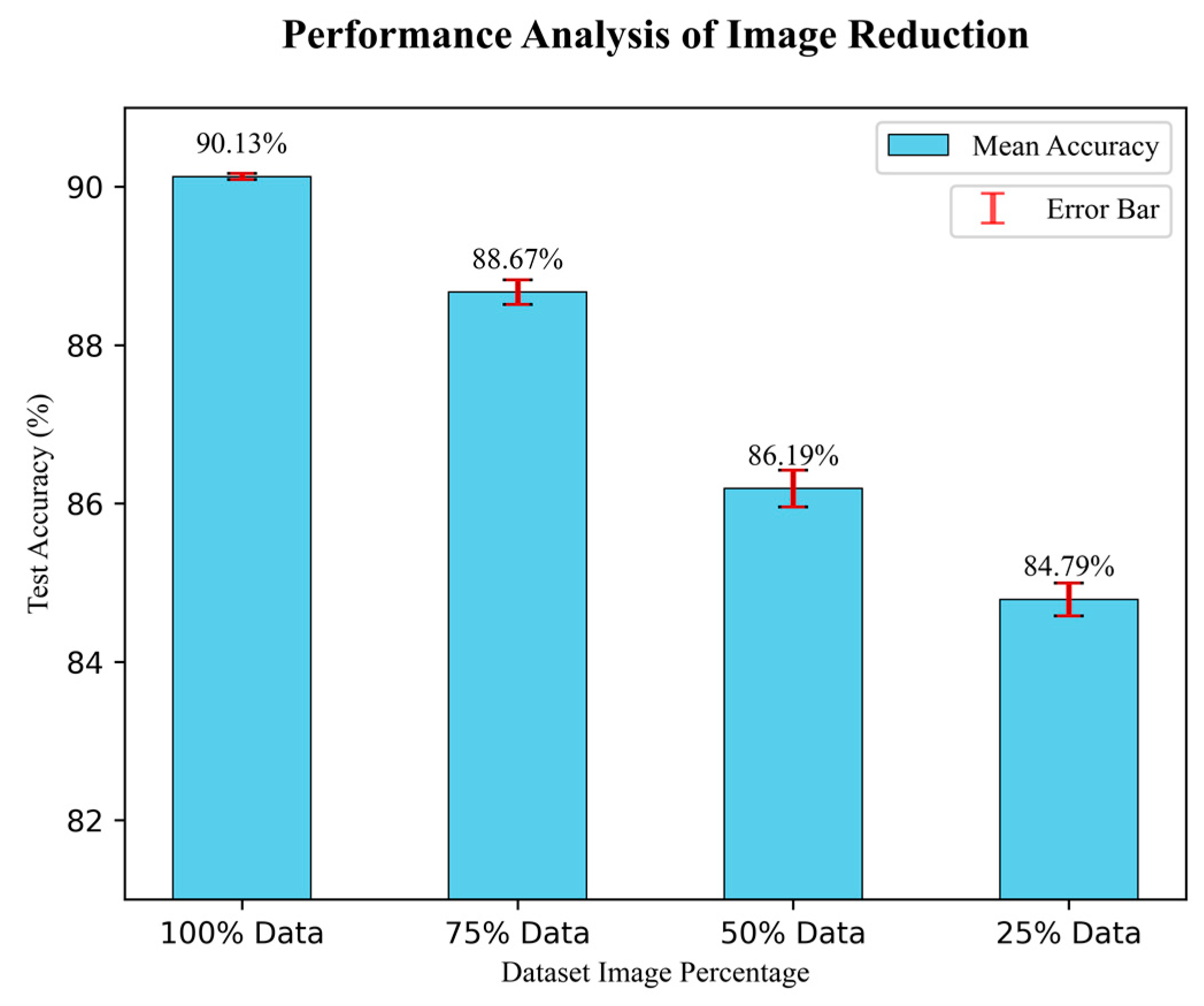
- To further examine the generalization capabilities and robustness of our model in relation to the size of the training dataset, the model is trained four times with a gradually decreasing number of images. Even with a smaller number of images, the model demonstrates good performance, demonstrating the robustness of the DR-CCTNet model.
2. Literature Review
3. Methodology
3.1. Dataset Description
3.2. Image Pre-Processing
3.2.1. Artifacts Removal
Otsu Thresholding
Contour Detection
Regions of Interest Extraction
3.2.2. Noise Eradication
Morphological Opening
Non-Local Means Denoising (NLMD)
3.2.3. Image Enhancement (CLAHE)
3.3. Data Balancing
3.3.1. Under Sampling
| Algorithm 1: Under Sampling |
| 1. Define class names class_names = [‘Grade 0’, ‘Grade 1’, ‘Grade 2, ‘Grade 3’, ‘Grade 4’] 2. Define image numbers for each class class_image_numbers = [7 ‘Grade 3’: 1441, ‘Grade 4’: 1987] 3. Calculate the average image numbers of the smaller three classes smallest_classes = [‘Grade 1’, ‘Grade 3’, ‘Grade 4’] Smaller classes image numbers = [class_image_numbers[class_names] for class_name in smaller_classes] average_image_numbers = int(np.mean(lower_classes_image_numbers)) 4. Random under sample the higher two classes to the average size Larger_classes = [‘Grade 0’, ‘Grade 2’] for class_name in larger_classes class_image_number = class_image_numbers[class_names] undersample_ratio = average_image_numbers/class_image_number undersampled_image_numbers = int(class_image_number × undersample_ratio) class_image_numbers[class_name] = undersampled_image_numbers |
3.3.2. Data Augmentation
3.4. Model Comparison
3.4.1. Training Strategy for Transfer Learning Models
3.4.2. Transfer Learning Models
VGG16
VGG19
ResNet50
MobileNetV2
3.4.3. Transformer Models
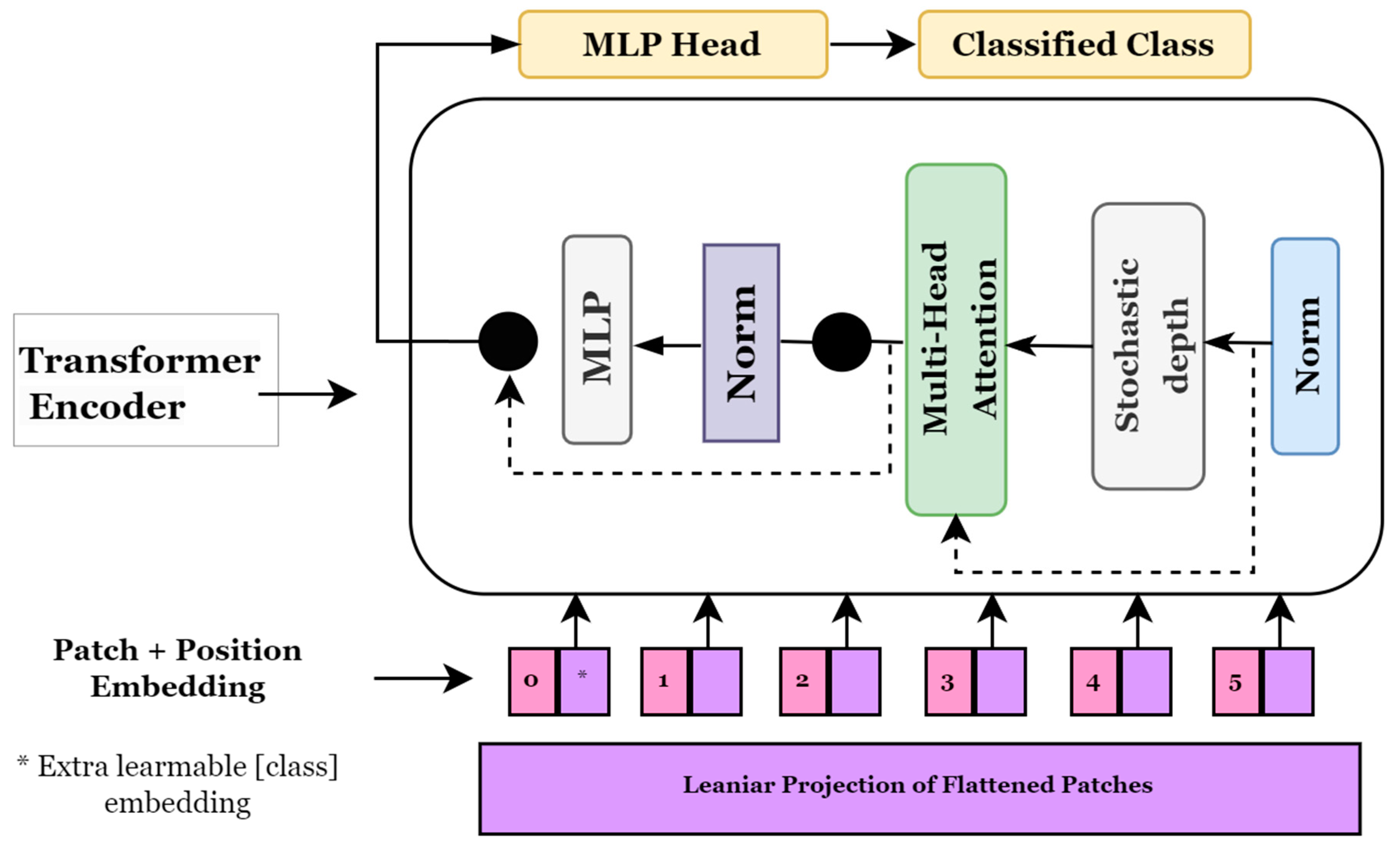
Vision Transformer (ViT)
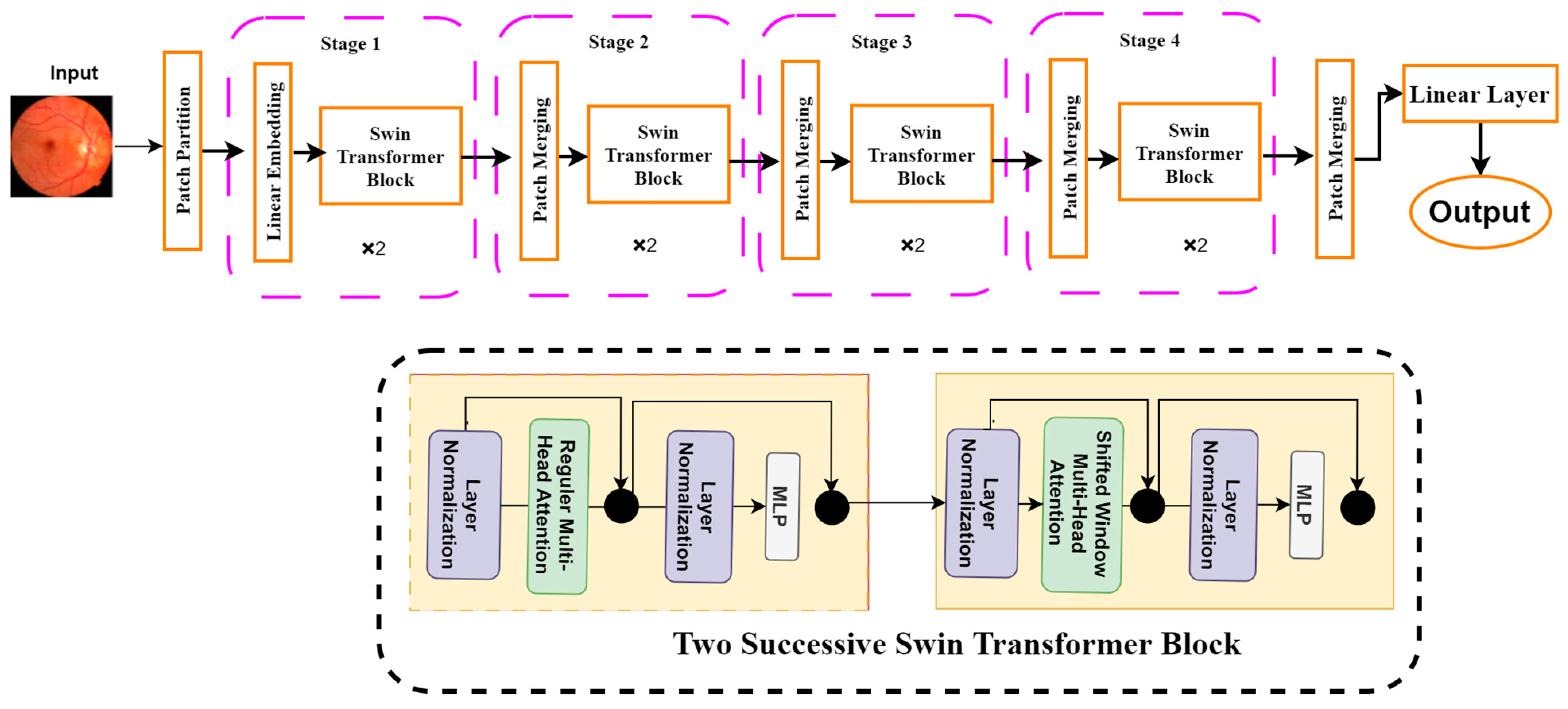
Shifted Window Transformers (Swin Transformers)
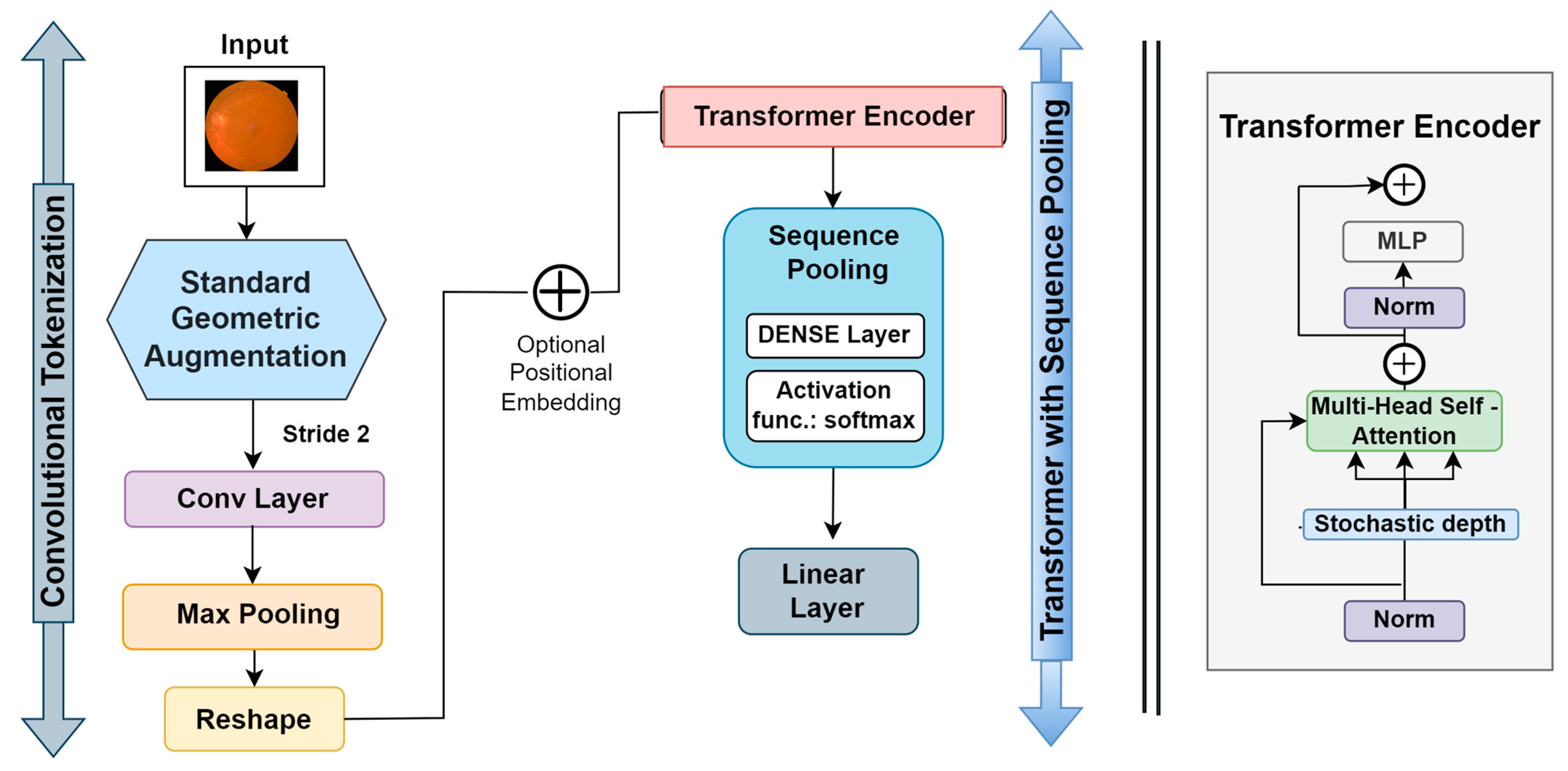
Compact convolutional transformer (CCT)
3.4.4. Results of the Transfer Learning and Transformer Models
3.5. Base Model
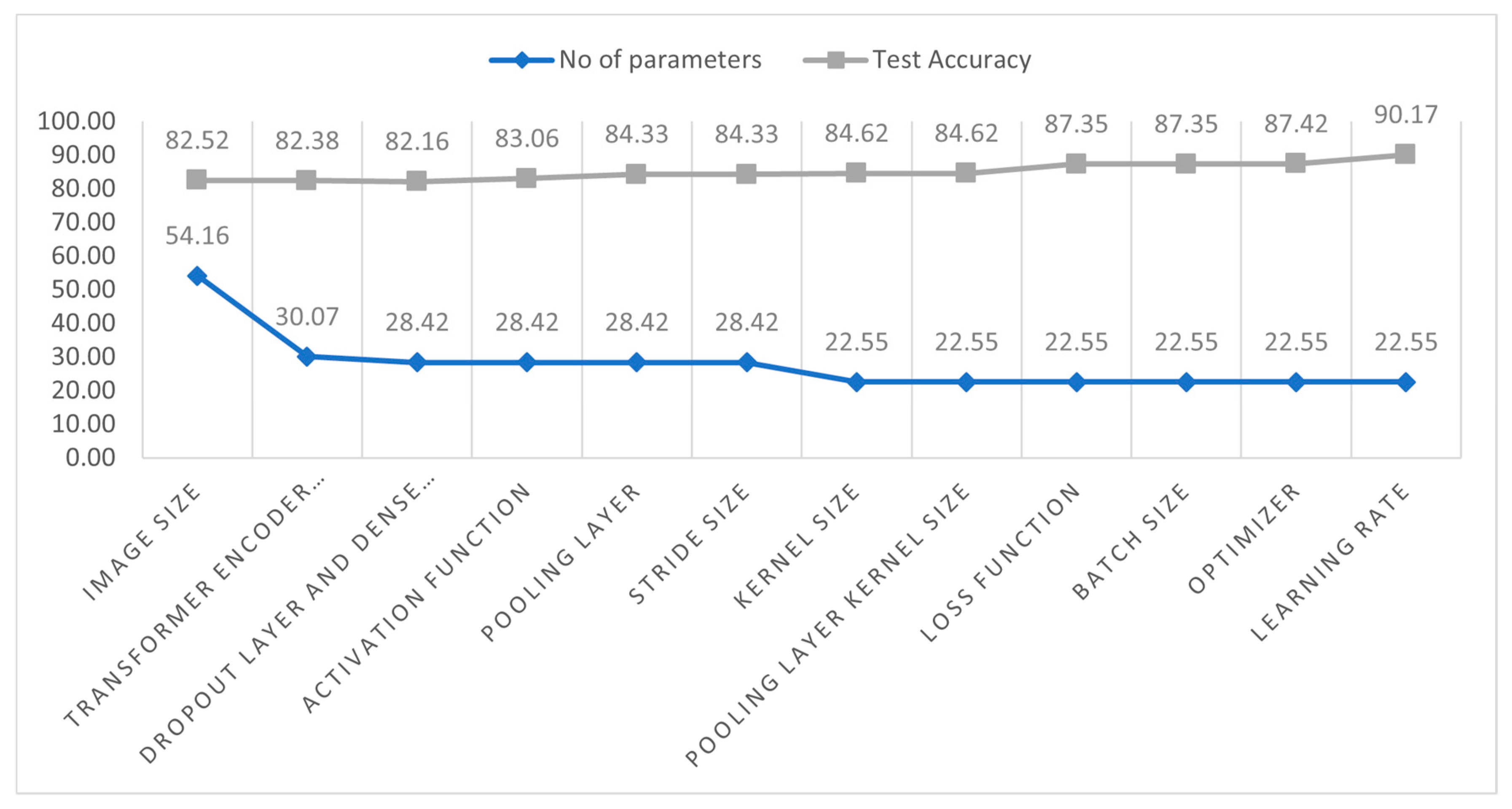
3.6. Ablation Study
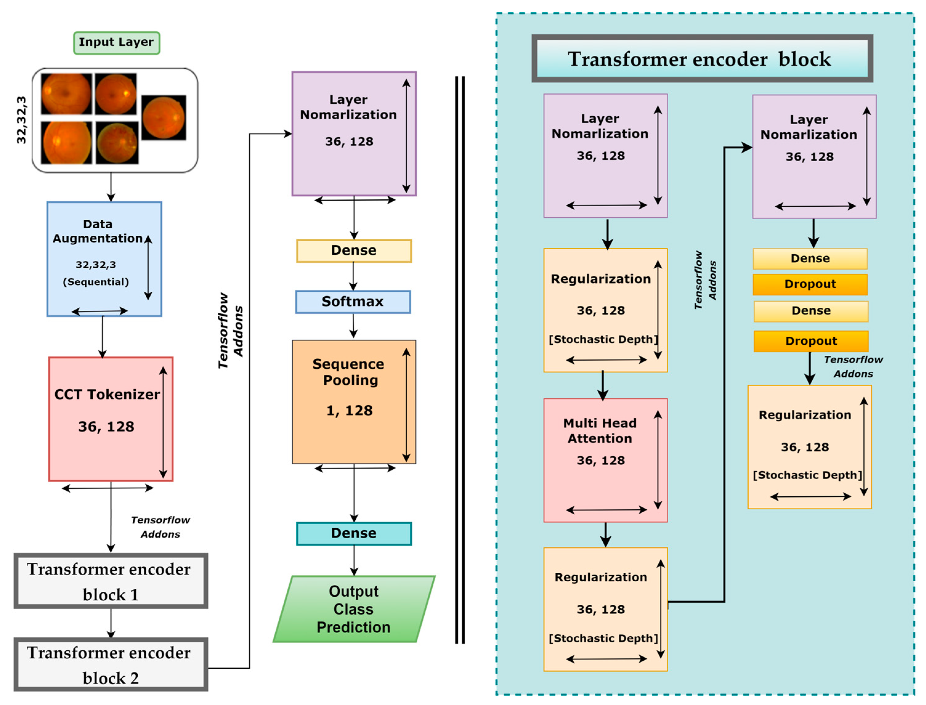
3.7. DR-CCTNet
4. Analysis of Results
4.1. Performance Metrics
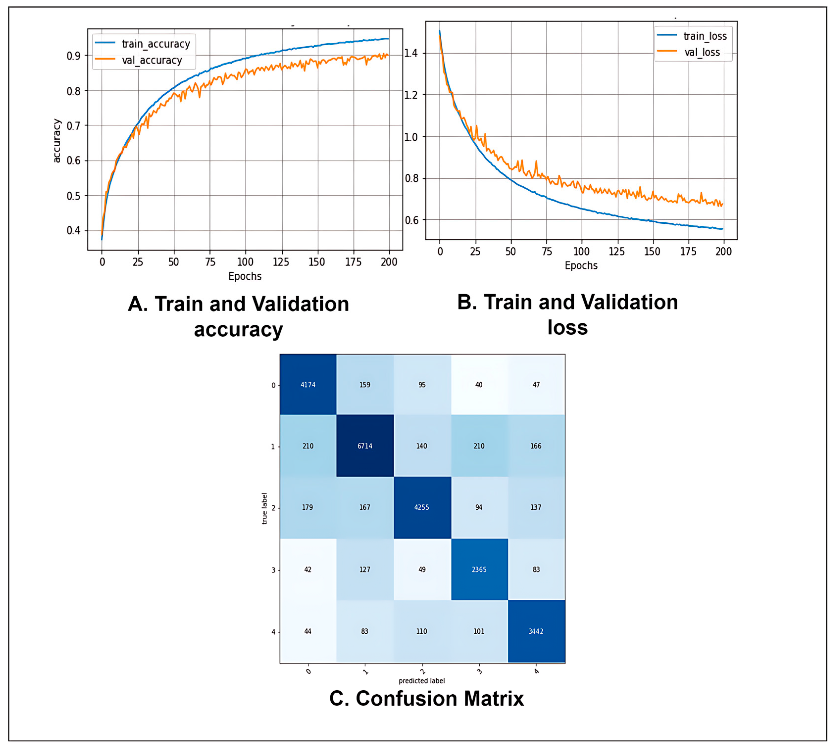
4.2. Performance Analysis of the Proposed Model
4.3. Analysis of Image Size Tuning
4.4. Analysis of the Performance with Image Reduction
5. Conclusions
6. Limitations and Future Research
Author Contributions
Funding
Institutional Review Board Statement
Informed Consent Statement
Data Availability Statement
Acknowledgments
Conflicts of Interest
References
- Wykoff, C.C.; Khurana, R.N.; Nguyen, Q.D.; Kelly, S.P.; Lum, F.; Hall, R.; Abbass, I.M.; Abolian, A.M.; Stoilov, I.; To, T.M. Risk of blindness among patients with diabetes and newly diagnosed diabetic retinopathy. Diabetes Care 2021, 44, 748–756. [Google Scholar] [CrossRef]
- Harris-Hayes, M.; Schootman, M.; Schootman, J.C.; Hastings, M.K. The role of physical therapists in fighting the type 2 diabetes epidemic. J. Orthop. Sport. Phys. Ther. 2020, 50, 5–16. [Google Scholar] [CrossRef] [PubMed]
- Shanthi, T.; Sabeenian, R. Modified Alexnet architecture for classification of diabetic retinopathy images. Comput. Electr. Eng. 2019, 76, 56–64. [Google Scholar] [CrossRef]
- Lanzetta, P.; Sarao, V.; Scanlon, P.H.; Barratt, J.; Porta, M.; Bandello, F.; Loewenstein, A. Fundamental principles of an effective diabetic retinopathy screening program. Acta Diabetol. 2020, 57, 785–798. [Google Scholar] [CrossRef] [PubMed]
- Alyoubi, W.L.; Shalash, W.M.; Abulkhair, M.F. Diabetic retinopathy detection through deep learning techniques: A review. Inform. Med. Unlocked 2020, 20, 100377. [Google Scholar] [CrossRef]
- Khan, I.U.; Azam, S.; Montaha, S.; Al Mahmud, A.; Rafid, A.R.H.; Hasan, M.Z.; Jonkman, M. An effective approach to address processing time and computational complexity employing modified CCT for lung disease classification. Intell. Syst. Appl. 2022, 16, 200147. [Google Scholar] [CrossRef]
- Sabbagh, F.; Muhamad, I.I.; Niazmand, R.; Dikshit, P.K.; Kim, B.S. Recent progress in polymeric non-invasive insulin delivery. Int. J. Biol. Macromol. 2022, 203, 222–243. [Google Scholar] [CrossRef]
- Hassani, A.; Walton, S.; Shah, N.; Abuduweili, A.; Li, J.; Shi, H. Escaping the big data paradigm with compact transformers. arXiv 2021, arXiv:2104.05704. [Google Scholar]
- Qureshi, I.; Ma, J.; Abbas, Q. Diabetic retinopathy detection and stage classification in eye fundus images using active deep learning. Multimed. Tools Appl. 2021, 80, 11691–11721. [Google Scholar] [CrossRef]
- Hemanth, D.J.; Deperlioglu, O.; Kose, U. An enhanced diabetic retinopathy detection and classification approach using deep convolutional neural network. Neural Comput. Appl. 2020, 32, 707–721. [Google Scholar] [CrossRef]
- Gu, Z.; Li, Y.; Wang, Z.; Kan, J.; Shu, J.; Wang, Q. Classification of Diabetic Retinopathy Severity in Fundus Images Using the Vision Transformer and Residual Attention. Comput. Intell. Neurosci. 2023, 2023, 1305583. [Google Scholar] [CrossRef] [PubMed]
- Qummar, S.; Khan, F.G.; Shah, S.; Khan, A.; Shamshirband, S.; Rehman, Z.U.; Khan, I.A.; Jadoon, W. A deep learning ensemble approach for diabetic retinopathy detection. IEEE Access 2019, 7, 150530–150539. [Google Scholar] [CrossRef]
- Liu, H.; Yue, K.; Cheng, S.; Pan, C.; Sun, J.; Li, W. Hybrid model structure for diabetic retinopathy classification. J. Healthc. Eng. 2020, 2020, 8840174. [Google Scholar] [CrossRef]
- Wu, Z.; Shi, G.; Chen, Y.; Shi, F.; Chen, X.; Coatrieux, G.; Yang, J.; Luo, L.; Li, S. Coarse-to-fine classification for diabetic retinopathy grading using convolutional neural network. Artif. Intell. Med. 2020, 108, 101936. [Google Scholar] [CrossRef]
- Lam, C.; Yi, D.; Guo, M.; Lindsey, T. Automated detection of diabetic retinopathy using deep learning. AMIA Summits Transl. Sci. Proc. 2018, 2018, 147. [Google Scholar]
- Gao, Z.; Li, J.; Guo, J.; Chen, Y.; Yi, Z.; Zhong, J. Diagnosis of diabetic retinopathy using deep neural networks. IEEE Access 2018, 7, 3360–3370. [Google Scholar] [CrossRef]
- APTOS 2019 Blindness Detection. Available online: https://www.kaggle.com/competitions/aptos2019-blindness-detection/data,2019 (accessed on 20 February 2023).
- Patry, G.G.; Gervais; Bruno, L.A.Y.; Roger, J.; Elie, D.; Foltete, M.; Donjon, A.; Maffre, H. Messidor-2. Available online: https://www.adcis.net/en/third-party/messidor2/ (accessed on 20 February 2023).
- Porwal, P.; Pachade, S.; Kamble, R.; Kokare, M.; Deshmukh, G.; Sahasrabuddhe, V.; Meriaudeau, F. Indian diabetic retinopathy image dataset (IDRiD): A database for diabetic retinopathy screening research. Data 2018, 3, 25. [Google Scholar] [CrossRef]
- Li, T.; Gao, Y.; Wang, K.; Guo, S.; Liu, H.; Kang, H. Diagnostic assessment of deep learning algorithms for diabetic retinopathy screening. Inf. Sci. 2019, 501, 511–522. [Google Scholar] [CrossRef]
- Diabetic Retinopathy Detection. Available online: https://www.kaggle.com/c/diabetic-retinopathy-detection (accessed on 20 February 2023).
- Rasta, S.H.; Partovi, M.E.; Seyedarabi, H.; Javadzadeh, A. A comparative study on preprocessing techniques in diabetic retinopathy retinal images: Illumination correction and contrast enhancement. J. Med. Signals Sens. 2015, 5, 40. [Google Scholar] [CrossRef]
- Pinedo-Diaz, G.; Ortega-Cisneros, S.; Moya-Sanchez, E.U.; Rivera, J.; Mejia-Alvarez, P.; Rodriguez-Navarrete, F.J.; Sanchez, A. Suitability Classification of Retinal Fundus Images for Diabetic Retinopathy Using Deep Learning. Electronics 2022, 11, 2564. [Google Scholar] [CrossRef]
- Goh, T.Y.; Basah, S.N.; Yazid, H.; Safar, M.J.A.; Saad, F.S.A. Performance analysis of image thresholding: Otsu technique. Measurement 2018, 114, 298–307. [Google Scholar] [CrossRef]
- Ming, Y.; Li, H.; He, X. Contour completion without region segmentation. IEEE Trans. Image Process. 2016, 25, 3597–3611. [Google Scholar] [CrossRef]
- Alban, M.; Gilligan, T. Automated detection of diabetic retinopathy using fluorescein angiography photographs. Rep. Standford Educ. 2016.
- Montaha, S.; Azam, S.; Rafid, A.K.M.R.H.; Ghosh, P.; Hasan, M.; Jonkman, M.; De Boer, F. BreastNet18: A high accuracy fine-tuned VGG16 model evaluated using ablation study for diagnosing breast cancer from enhanced mammography images. Biology 2021, 10, 1347. [Google Scholar] [CrossRef] [PubMed]
- Raiaan, M.A.K.; Fatema, K.; Khan, I.U.; Azam, S.; Rashid, R.U.; Mukta, S.H.; Jonkman, M.; De Boer, F. A Lightweight Robust Deep Learning Model Gained High Accuracy in Classifying a Wide Range of Diabetic Retinopathy Images. IEEE Access 2023, 11, 42361–42388. [Google Scholar] [CrossRef]
- Shao, F.; Yang, Y.; Jiang, Q.; Jiang, G.; Ho, Y.-S. Automated quality assessment of fundus images via analysis of illumination, naturalness and structure. IEEE Access 2017, 6, 806–817. [Google Scholar] [CrossRef]
- Nie, Y.; Zamzam, A.S.; Brandt, A. Resampling and data augmentation for short-term PV output prediction based on an imbalanced sky images dataset using convolutional neural networks. Sol. Energy 2021, 224, 341–354. [Google Scholar] [CrossRef]
- Hussain, Z.; Gimenez, F.; Yi, D.; Rubin, D. Differential data augmentation techniques for medical imaging classification tasks. AMIA Annu. Symp. Proc. 2017, 2017, 979–984. [Google Scholar] [PubMed]
- Shazia, A.; Xuan, T.Z.; Chuah, J.H.; Usman, J.; Qian, P.; Lai, K.W. A comparative study of multiple neural network for detection of COVID-19 on chest X-ray. EURASIP J. Adv. Signal Process. 2021, 2021, 50. [Google Scholar] [CrossRef]
- Fahad, N.M.; Sakib, S.; Raiaan, M.A.K.; Mukta, M.S.H. SkinNet-8: An Efficient CNN Architecture for Classifying Skin Cancer on an Imbalanced Dataset. In Proceedings of the 2023 International Conference on Electrical, Computer and Communication Engineering (ECCE), Chittagong, Bangladesh, 23–25 February 2023; pp. 1–6. [Google Scholar]
- Fatema, K.; Montaha, S.; Rony, M.A.H.; Azam, S.; Hasan, M.Z.; Jonkman, M. A Robust Framework Combining Image Processing and Deep Learning Hybrid Model to Classify Cardiovascular Diseases Using a Limited Number of Paper-Based Complex ECG Images. Biomedicines 2022, 10, 2835. [Google Scholar] [CrossRef] [PubMed]
- Vaswani, A.; Shazeer, N.; Parmar, N.; Uszkoreit, J.; Jones, L.; Gomez, A.N.; Kaiser, Ł.; Polosukhin, I. Attention is all you need. Adv. Neural Inf. Process. Syst. 2017, 30. [Google Scholar]
- Islam, M.N.; Hasan, M.; Hossain, M.K.; Alam, M.G.R.; Uddin, M.Z.; Soylu, A. Vision transformer and explainable transfer learning models for auto detection of kidney cyst, stone and tumor from CT-radiography. Sci. Rep. 2022, 12, 11440. [Google Scholar] [CrossRef] [PubMed]
- Dosovitskiy, A.; Beyer, L.; Kolesnikov, A.; Weissenborn, D.; Zhai, X.; Unterthiner, T.; Dehghani, M.; Minderer, M.; Heigold, G.; Gelly, S. An image is worth 16x16 words: Transformers for image recognition at scale. arXiv 2020, arXiv:2010.11929. [Google Scholar]
- Lin, T.-Y.; Dollár, P.; Girshick, R.; He, K.; Hariharan, B.; Belongie, S. Feature pyramid networks for object detection. In Proceedings of the IEEE conference on computer vision and pattern recognition, Honolulu, HI, USA, 21–26 July 2017; pp. 2117–2125. [Google Scholar]
- Ronneberger, O.; Fischer, P.; Brox, T. U-net: Convolutional networks for biomedical image segmentation. In Proceedings of the Medical Image Computing and Computer-Assisted Intervention–MICCAI 2015: 18th International Conference, Munich, Germany, 5–9 October 2015; Proceedings, Part III 18, 2015. pp. 234–241. [Google Scholar]


| Paper | Model | Datasets | Number of Image | Image Size (Pixels) |
|---|---|---|---|---|
| Shanthi et al. [3] | Modified AlexNet | Messidor | 1190 | 259 × 259 |
| Hemanth et al. [10] | Proposed CNN model | MESSIDOR | 400 | 150× 255 |
| Gu et al. [11] | Proposed transformer model by using vision transformers and residual attention | DDR and IDRiD | 13,673 and 516 | 512 × 512 |
| Sehrish et al. [12] | Ensemble Classifier | DR’s Kaggle dataset | 35,126 | 512 × 512 |
| Liu et al. [13] | Hybrid deep learning model | DeepDR, APOTS, and EyePACS | 1200, 3662 and 35,126 | 380 × 380 |
| Wu et al. [14] | CF-DRNet | IDRiD and DR’s Kaggle dataset | 413 and 35,126 | 256 × 256 |
| Lam et al. [15] | CNN based architectures | DR’s Kaggle dataset and Messidor-1 | 35,126 and 1090 | 256 × 256 |
| Gao et al. [16] | Inception@4 | DR Fundus | 4476 | 600 × 600 |
| Datasets | Messidor2 | APTOS | IDRiD | Diabetic Retinopathy | DDR | Merge |
|---|---|---|---|---|---|---|
| No DR (0) | 1017 | 1805 | 134 | 25,810 | 6265 | 34,830 |
| Mild NPDR (1) | 270 | 370 | 20 | 2443 | 630 | 3718 |
| Moderate NPDR (2) | 347 | 999 | 136 | 5292 | 4447 | 11,209 |
| Severe NPDR (3) | 75 | 193 | 74 | 873 | 236 | 1441 |
| PDR (4) | 35 | 295 | 49 | 708 | 913 | 1987 |
| Total Images | 1744 | 3662 | 413 | 35,126 | 12,491 | 53,185 |
| Grade | Merge | Under Sampling | After Augmentation |
|---|---|---|---|
| 0 | 34,830 | 2384 | 30,992 |
| 1 | 3718 | 3718 | 48,334 |
| 2 | 11,209 | 2384 | 30,992 |
| 3 | 1441 | 1441 | 18,733 |
| 4 | 1987 | 1987 | 25,831 |
| Total | 53,185 | 11,914 | 154,882 |
| Model Name | Image Size | Accuracy | Epoch × Time |
|---|---|---|---|
| MobileNetV2 | 32 × 32 | 71.98% | 195 × 386 s |
| VGG16 | 32 × 32 | 73.22% | 165 × 391 s |
| VGG19 | 32 × 32 | 72.88% | 177 × 404 s |
| ResNet50 | 32 × 32 | 76.67% | 142 × 423 s |
| Swin Transformer | 32 × 32 | 82.23% | 200 × 95 s |
| Vit | 32 × 32 | 81.56% | 200 ×104 s |
| CCT | 32 × 32 | 84.52% | 200 × 78 s |
| Study 1: Changing Image Size | |||||
| Configuration No. | Image Size | No. of Parameters | Epoch | Training Time | Test Accuracy (%) |
| 1 | 32 × 32 (Base model) | 5,41,638 | 200 | 78 s | 84.88% |
| 2 | 28 × 28 | 541,638 | 200 | 60 s | 83.91% |
| 3 | 24 × 24 | 541,638 | 200 | 48 s | 83.23% |
| 4 | 16 × 16 | 541,638 | 200 | 38 s | 82.52% |
| Study 2: Changing the Transformer Encoder Block | |||||
| Configuration No. | No of transformer encoder blocks | No. of Parameters | Epoch | training time | Test accuracy (%) |
| 1 | 3 | 707,142 | 200 | 70 s | 82.88 |
| 2 | 2 | 541,638 | 200 | 38 s | 82.52 |
| 3 | 1 | 300,678 | 200 | 21 s | 82.38 |
| Study 3: Changing the Dropout Layer and Dense Layer | |||||
| Configuration No. | No of dropout layer | No of dense layer | No. of Parameters | Epoch × training time | Test accuracy (%) |
| 1 | 3 | 3 | 317,190 | 200 × 21 s | 82.42 |
| 2 | 2 | 2 | 300,678 | 200 × 20 s | 82.38 |
| 3 | 1 | 1 | 284,166 | 200 × 19 s | 82.16 |
| Study 4: Changing the activation function | |||||
| Configuration No. | Activation function | No. of parameters | Epoch × training time | Test accuracy (%) | Findings |
| 1 | Tanh | 284,166 | 200 × 19 s | 82.16 | Previous accuracy |
| 2 | relu | 284,166 | 200 × 19 s | 83.06 | Highest Accuracy |
| 3 | elu | 284,166 | 200 × 19 s | 82.38 | Accuracy improved |
| 4 | softsign | 284,166 | 200 × 19 s | 76.40 | Accuracy dropped |
| 5 | softplus | 284,166 | 200 × 19 s | 75.97 | Accuracy dropped |
| Study 5: Changing the pooling layer | |||||
| Configuration No. | Type of pooling layer | No of parameters | Epoch × training time | Test accuracy (%) | Findings |
| 1 | Max | 284,166 | 200 × 19 s | 84.33 | Highest Accuracy |
| 2 | Average | 284,166 | 200 × 19 s | 83.06 | Previous accuracy |
| Study 6: Changing the stride size | |||||
| Configuration No. | No. of strides | No. of Parameters | Epoch × training time | Test accuracy (%) | Findings |
| 1 | 1 | 284,166 | 200 × 19 s | 84.33 | Previous Accuracy |
| 2 | 2 | 284,166 | 200 × 19 s | 83.16 | Accuracy dropped |
| 3 | 3 | 284,166 | 200 × 19 s | 82.97 | Accuracy dropped |
| 4 | 4 | 284,166 | 200 × 19 s | 81.43 | Accuracy dropped |
| Study 7: Changing the Kernel Size | |||||
| Configuration No. | No. of Kernel Size | No. of Parameter | Epoch × Training Time | Test Accuracy (%) | Finding |
| 1 | 4 | 284,166 | 200 × 19 s | 84.33 | Previous accuracy |
| 2 | 3 | 225,478 | 200 × 16 s | 84.62 | Highest Accuracy |
| 3 | 2 | 183,558 | 200 × 13 s | 80.12 | Accuracy dropped |
| 4 | 1 | 158,406 | 200 × 11 s | 76.31 | Accuracy dropped |
| Study 8: Changing the kernel size of the pooling layer | |||||
| Configuration No. | No. of pooling kernel size | No. of Parameter | Epoch × training time | Test accuracy (%) | Finding |
| 1 | 5 | 225,478 | 200 × 16 s | 84.57 | Accuracy dropped |
| 2 | 4 | 225,478 | 200 × 16 s | 85.12 | Accuracy improved |
| 3 | 3 | 225,478 | 200 × 16 s | 85.68 | Highest Accuracy |
| 4 | 2 | 225,478 | 200 × 16 s | 84.62 | Previous accuracy |
| 5 | 1 | 225,478 | 200 × 16 s | 83.9 | Accuracy dropped |
| Study 9: Changing the loss function | |||||
| Configuration No. | Loss Function | No. of Parameter | Epoch × training time | Test accuracy (%) | Finding |
| 1 | Binary Cross-entropy | 225,478 | 200 × 16 s | 87.12 | Accuracy improved |
| 2 | Categorical Cross-entropy | 225,478 | 200 × 16 s | 87.35 | Highest Accuracy |
| 3 | Mean Squared Error | 225,478 | 200 × 16 s | 85.68 | Previous accuracy |
| 4 | Mean absolute error | 225,478 | 200 × 16 s | 84.93 | Accuracy dropped |
| 5 | Mean squared logarithmic error | 225,478 | 200 × 16 s | 85.76 | Accuracy dropped |
| Study 10: Changing the batch size | |||||
| Configuration No. | Batch size | No. of Parameter | Epoch × training time | Test accuracy (%) | Finding |
| 1 | 256 | 225,478 | 200 × 12 s | 86.88 | Accuracy dropped |
| 2 | 128 | 225,478 | 200 × 16 s | 87.35 | Previous accuracy |
| 3 | 64 | 225,478 | 200 × 22 s | 87.53 | Accuracy improved |
| 4 | 32 | 225,478 | 200 × 31 s | 87.78 | Accuracy improved |
| Study 11: Changing the optimizer | |||||
| Configuration No. | Optimizer | No. of Parameter | Epoch × training time | Test accuracy (%) | Finding |
| 1 | Adam | 225,478 | 200 × 16 s | 87.42 | Highest Accuracy |
| 2 | Nadam | 225,478 | 200 × 16 s | 86.78 | Accuracy dropped |
| 3 | SGD | 225,478 | 200 × 16 s | 87.35 | Previous accuracy |
| 4 | Adamax | 225,478 | 200 × 16 s | 84.18 | Accuracy dropped |
| 5 | RMSprop | 225,478 | 200 × 16 s | 86.8 | Accuracy dropped |
| Study 12: Changing the learning rate | |||||
| Configuration No. | Learning rate | No. of Parameter | Epoch × training time | Test accuracy (%) | Finding |
| 1 | 0.01 | 225,478 | 200 × 16 s | 86.12 | Accuracy dropped |
| 2 | 0.006 | 225,478 | 200 × 16 s | 87.42 | Previous accuracy |
| 3 | 0.001 | 225,478 | 200 × 16 s | 90.17 | Highest Accuracy |
| 4 | 0.0008 | 225,478 | 200 × 16 s | 89.8 | Accuracy improved |
| Configuration | Value |
|---|---|
| Image size | 16 × 16 |
| Epochs | 100 |
| Optimization function | Adam |
| Learning rate | 0.001 |
| Batch size | 256 |
| Kernel size | 3 |
| Activation function | ReLU |
| Loss Function | Categorical Cross-Entropy |
| Kernel size of the pooling layer | 3 |
| Stride size | 1 |
| Pooling layer | Max pooling |
| Projection_dim | 128 |
| Stochastic_depth_rate | 0.1 |
| Weight_decay | 0.001 |
| Measure | Value |
|---|---|
| Recall | 90.10% |
| Specificity | 97.51% |
| Precision | 89.38% |
| F1 Score (F1) | 89.72% |
| Fall-out or False Positive Rate (FPR) | 0.02492 |
| Miss Rate or False Negative Rate (FNR) | 0.09526 |
| False Discovery Rate (FDR) | 0.10618 |
| Negative Predictive Value (NPV) | 97.46% |
| Matthews Correlation Coefficient (MCC) | 87.22% |
| No. of Parameters | Image Size | Accuracy | Epoch × Time |
|---|---|---|---|
| 225,478 | 32 × 32 | 93.81% | 200 × 32 s |
| 225,478 | 28 × 28 | 93.33% | 200 × 28 s |
| 225,478 | 24 × 24 | 91.12% | 200 × 23 s |
| 225,478 | 16 × 16 | 90.17% | 200 × 16 s |
Disclaimer/Publisher’s Note: The statements, opinions and data contained in all publications are solely those of the individual author(s) and contributor(s) and not of MDPI and/or the editor(s). MDPI and/or the editor(s) disclaim responsibility for any injury to people or property resulting from any ideas, methods, instructions or products referred to in the content. |
© 2023 by the authors. Licensee MDPI, Basel, Switzerland. This article is an open access article distributed under the terms and conditions of the Creative Commons Attribution (CC BY) license (https://creativecommons.org/licenses/by/4.0/).
Share and Cite
Khan, I.U.; Raiaan, M.A.K.; Fatema, K.; Azam, S.; Rashid, R.u.; Mukta, S.H.; Jonkman, M.; De Boer, F. A Computer-Aided Diagnostic System to Identify Diabetic Retinopathy, Utilizing a Modified Compact Convolutional Transformer and Low-Resolution Images to Reduce Computation Time. Biomedicines 2023, 11, 1566. https://doi.org/10.3390/biomedicines11061566
Khan IU, Raiaan MAK, Fatema K, Azam S, Rashid Ru, Mukta SH, Jonkman M, De Boer F. A Computer-Aided Diagnostic System to Identify Diabetic Retinopathy, Utilizing a Modified Compact Convolutional Transformer and Low-Resolution Images to Reduce Computation Time. Biomedicines. 2023; 11(6):1566. https://doi.org/10.3390/biomedicines11061566
Chicago/Turabian StyleKhan, Inam Ullah, Mohaimenul Azam Khan Raiaan, Kaniz Fatema, Sami Azam, Rafi ur Rashid, Saddam Hossain Mukta, Mirjam Jonkman, and Friso De Boer. 2023. "A Computer-Aided Diagnostic System to Identify Diabetic Retinopathy, Utilizing a Modified Compact Convolutional Transformer and Low-Resolution Images to Reduce Computation Time" Biomedicines 11, no. 6: 1566. https://doi.org/10.3390/biomedicines11061566