
A Systematic Review and Meta-Analysis of Cerebrospinal Fluid Amyloid and Tau Levels Identifies Mild Cognitive Impairment Patients Progressing to Alzheimer’s Disease


Abstract
:1. Introduction
1.1. Alzheimer’s Disease in Context
1.2. Early-Stage Diagnosis of AD
1.3. Current Status of AD Diagnosis versus AD Prediction
1.4. Usage of Biomarkers in Prediction and Diagnosis of AD
1.5. Overview of Study
2. Materials and Methods
2.1. Search Strategy
2.2. Inclusion and Exclusion Criteria
2.3. Statistical Analysis
2.4. Use of Diagnostic Criteria to Define MCI and AD
3. Results
3.1. Methods to Determine Analyte Concentration in CSF
3.2. Baseline CSF Biomarker Measurements
3.3. Aβ1-42/T-Tau and Aβ1-42/P-Tau Ratio
3.4. Follow-Up Duration
3.5. Meta Analysis of Studies Investigating the Association between Levels of Amyloid Beta and Tau in CSF, and Progression to Alzheimer’s Disease
4. Discussion
4.1. Limitations of Current Study
4.2. The Effect of Follow-Up Length
Supplementary Materials
Author Contributions
Funding
Institutional Review Board Statement
Informed Consent Statement
Data Availability Statement
Conflicts of Interest
Appendix A. Meta-Analyses of Three Cerebrospinal Fluid Markers in Stable_MCI, MCI_AD, and HC
Appendix A.1. Software and Methodology
Appendix A.1.1. Required Software
Appendix A.1.2. Meta-Analysis Approach
Effect Measure
Models and Significance Tests for Overall Effects
Measurements and Tests of Between-Study Heterogeneity
Normality Assumptions
Bias Analysis
Summary Plot of the Meta-Analysis Results
Appendix A.2. Amyloid
| data <- read.csv(“sheet_Amyloid_3groups.csv”, as.is=TRUE) |
Appendix A.2.1. Stable MCI (MCI_St) versus MCI_AD
Models and Significance Tests for Overall Effect and Between-Study Heterogeneity
| meta <- metacont(N.MCI_St, Mean.MCI_St, SD.MCI_St, N.MCI_AD, Mean.MCI_AD, SD.MCI_AD, |
| sm=“SMD”, data=data, studlab=paste(Author, Year)) |
| meta$label.e <- “MCI_St” |
| meta$label.c <- “MCI_AD” |
| print(meta, digits=2) |
| ## SMD 95%-CI %W(fixed) %W(random) |
| ## Bjerke 2009 1.70 [ 1.11; 2.28] 2.1 4.3 |
| ## Mattsson 2009 0.54 [ 0.38; 0.69] 30.4 5.7 |
| ## Hertze 2010 0.90 [ 0.53; 1.26] 5.5 5.1 |
| ## Palmqvist 2012 1.46 [ 1.04; 1.87] 4.2 4.9 |
| ## Spencer 2019 0.76 [ 0.45; 1.06] 8.0 5.3 |
| ## Hansson 2006 1.50 [ 1.08; 1.92] 4.2 4.9 |
| ## Hansson 2007 1.03 [ 0.63; 1.43] 4.6 5.0 |
| ## Hampel 2004 0.79 [ 0.22; 1.36] 2.3 4.3 |
| ## Herukka 2007 0.85 [ 0.38; 1.32] 3.4 4.7 |
| ## Lanari 2009 1.30 [ 0.66; 1.94] 1.8 4.1 |
| ## Papaliagkas 2009 1.09 [ 0.15; 2.04] 0.8 3.0 |
| ## Eckerstrom 2010 1.26 [ 0.50; 2.02] 1.3 3.6 |
| ## Kester 2011 0.93 [ 0.51; 1.35] 4.2 4.9 |
| ## Seppala 2011 0.81 [ 0.21; 1.41] 2.0 4.2 |
| ## Buchhave 2012 1.93 [ 1.47; 2.39] 3.4 4.8 |
| ## Parnetti 2012 3.46 [ 2.79; 4.14] 1.6 3.9 |
| ## Prestia 2013 1.14 [ 0.49; 1.79] 1.7 4.0 |
| ## Leuzy 2015 0.70 [-0.03; 1.44] 1.4 3.7 |
| ## Baldeiras 2018 1.21 [ 0.85; 1.56] 5.8 5.2 |
| ## Khoonsari 2019 1.64 [ 1.07; 2.21] 2.2 4.3 |
| ## Santangelo 2020 0.78 [ 0.32; 1.25] 3.4 4.7 |
| ## Eckerstrom 2020 0.94 [ 0.58; 1.30] 5.7 5.2 |
| ## |
| ## Number of studies combined: k = 22 |
| ## Number of observations: o = 2581 |
| ## |
| ## SMD 95%-CI z p-value |
| ## Fixed effect model 0.97 [0.88; 1.05] 22.18 < 0.0001 |
| ## Random effects model 1.19 [0.96; 1.42] 10.10 < 0.0001 |
| ## |
| ## Quantifying heterogeneity: |
| ## tau^2 = 0.2360; tau = 0.4858; I^2 = 83.8% [76.6%; 88.8%]; H = 2.48 [2.07; 2.98] |
| ## |
| ## Test of heterogeneity: |
| ## Q d.f. p-value |
| ## 129.49 21 < 0.0001 |
| ## ##Details on meta-analytical method: |
| ## - Inverse variance method |
| ## - DerSimonian-Laird estimator for tau^2 |
| ## - Hedges’ g (bias corrected standardised mean difference) |
Normality Assumptions
| hist(meta$TE, xlim=c(0,4), breaks=12, cex.main=0.9, main=“Histogram of standardised |
| mean difference”, xlab=“Standardised mean difference (SMD)”) |

Bias Analysis
funnel(meta)

Summary Plot of the Meta-Analysis Results
| pdf(file=“forest_Amyloid_MCI_StvsMCI_AD.pdf”, paper=“a4r”) |
| forest(meta, xlab=“Standardised difference in mean response (MCI_St - MCI_AD)”, |
| xlab.pos=-20, smlab.pos=-20, fontsize =5) |
| dev.off() |
Appendix A.2.2. HC versus MCI_AD
Models and Significance Tests for Overall Effect and Between-Study Heterogeneity
| meta <- metacont(N.HC, Mean.HC, SD.HC, N.MCI_AD, Mean.MCI_AD, SD.MCI_AD, sm=“SMD”, |
| data=data, studlab=paste(Author, Year)) |
| ## Warning in metacont(N.HC, Mean.HC, SD.HC, N.MCI_AD, Mean.MCI_AD, SD.MCI_AD, : |
| ## Note, studies with non-positive values for n.e and / or n.c get no weight in |
| ## meta-analysis. |
| meta$label.e <- “HC” |
| meta$label.c <- “MCI_AD” |
| print(meta, digits=2) |
| ## SMD 95%-CI %W(fixed) %W(random) |
| ## Bjerke 2009 3.40 [2.63; 4.16] 2.5 6.9 |
| ## Mattsson 2009 1.31 [1.13; 1.49] 44.8 10.4 |
| ## Hertze 2010 1.54 [1.06; 2.01] 6.4 8.9 |
| ## Palmqvist 2012 NA 0.0 0.0 |
| ## Spencer 2019 NA 0.0 0.0 |
| ## Hansson 2006 2.68 [2.12; 3.25] 4.6 8.3 |
| ## Hansson 2007 1.66 [1.18; 2.15] 6.1 8.8 |
| ## Hampel 2004 1.95 [1.10; 2.80] 2.0 6.4 |
| ## Herukka 2007 1.43 [0.96; 1.90] 6.5 8.9 |
| ## Lanari 2009 NA 0.0 0.0 |
| ## Papaliagkas 2009 NA 0.0 0.0 |
| ## Eckerstrom 2010 0.77 [0.16; 1.38] 3.9 7.9 |
| ## Kester 2011 NA 0.0 0.0 |
| ## Seppala 2011 1.03 [0.31; 1.75] 2.8 7.2 |
| ## Buchhave 2012 2.47 [1.96; 2.98] 5.6 8.6 |
| ## Parnetti 2012 NA 0.0 0.0 |
| ## Prestia 2013 NA 0.0 0.0 |
| ## Leuzy 2015 NA 0.0 0.0 |
| ## Baldeiras 2018 1.36 [0.99; 1.74] 10.4 9.5 |
| ## Khoonsari 2019 1.51 [0.93; 2.09] 4.3 8.2 |
| ## Santangelo 2020 NA 0.0 0.0 |
| ## Eckerstrom 2020 NA 0.0 0.0 |
| ## |
| ## Number of studies combined: k = 12 |
| ## |
| Number of observations: o = 1855 |
| ## |
| ## SMD 95%-CI z p-value |
| ## Fixed effect model 1.53 [1.41; 1.65] 24.86 < 0.0001 |
| ## Random effects model 1.73 [1.39; 2.07] 9.98 < 0.0001 |
| ## |
| ## Quantifying heterogeneity: |
| ## tau^2 = 0.2799; tau = 0.5291; I^2 = 83.7% [72.9%; 90.1%]; H = 2.47 [1.92; 3.19] |
| ## |
| ## Test of heterogeneity: |
| ## Q d.f. p-value |
| ## 67.35 11 < 0.0001 |
| ## |
| ## Details on meta-analytical method: |
| ## - Inverse variance method |
| ## - DerSimonian-Laird estimator for tau^2 |
| ## - Hedges’ g (bias corrected standardised mean difference) |
Normality Assumptions
| hist(meta$TE, xlim=c(0,4), breaks=12, cex.main=0.9, main=“Histogram of standardised mean difference”, xlab=“Standardised mean difference (SMD)”) |

Bias Analysis
	     funnel
        (meta)

Summary Plot of the Meta-Analysis Results
| pdf(file=“forest_Amyloid_HCvsMCI_AD.pdf”, paper=“a4r”) |
| forest(meta, xlab=“Standardised difference in mean response (HC - MCI_AD)”, |
| xlab.pos=-20, smlab.pos=-20, fontsize = 5) |
| dev.off() |
Appendix A.3. T-Tau
data <- read.csv(“sheet_Ttau_3groups.csv”, as.is=TRUE)
Appendix A.3.1. Stable MCI (MCI_St) versus MCI_AD
Models and Significance Tests for Overall Effect and Between-Study Heterogeneity
| meta <- metacont(N.MCI_St, Mean.MCI_St, SD.MCI_St, N.MCI_AD, Mean.MCI_AD, SD.MCI_AD, |
| sm=“SMD”, data=data, studlab=paste(Author, Year)) |
| ## Warning in metacont(N.MCI_St, |
| Mean.MCI_St, SD.MCI_St, N.MCI_AD, Mean.MCI_AD, : |
| ## Note, studies with non-positive values for n.e and / or n.c get no weight in |
| ## meta-analysis. |
| meta$label.e <- “MCI_St” |
| meta$label.c <- “MCI_AD” |
| print(meta, digits=2) |
| ## SMD 95%-CI %W(fixed) %W(random) ## Bjerke 2009 -0.74 [-1.27; -0.21] 2.8 4.8 |
| ## Mattsson 2009 -0.95 [-1.11; -0.79] 30.3 6.6 |
| ## Hertze 2010 -1.09 [-1.46; -0.72] 5.7 5.6 |
| ## Palmqvist 2012 -1.08 [-1.48; -0.69] 5.0 5.5 |
| ## Spencer 2019 -0.32 [-0.62; -0.03] 9.0 6.0 |
| ## Hansson 2006 -1.40 [-1.81; -0.99] 4.6 5.4 |
| ## Hansson 2007 NA 0.0 0.0 |
| ## Hampel 2004 -0.29 [-0.84; 0.26] 2.6 4.7 |
| ## Herukka 2007 -1.19 [-1.67; -0.70] 3.3 5.0 |
| ## Lanari 2009 -0.62 [-1.21; -0.02] 2.2 4.4 |
| ## Papaliagkas 2009 NA 0.0 0.0 |
| ## Eckerstrom 2010 -1.14 [-1.89; -0.39] 1.4 3.7 |
| ## Kester 2011 -1.12 [-1.54; -0.69] 4.3 5.3 |
| ## Seppala 2011 -1.19 [-1.82; -0.56] 2.0 4.2 |
| ## Buchhave 2012 -1.22 [-1.64; -0.81] 4.5 5.4 |
| ## Parnetti 2012 -2.99 [-3.61; -2.37] 2.0 4.3 |
| ## Prestia 2013 NA 0.0 0.0 |
| ## Leuzy 2015 -0.40 [-1.12; 0.31] 1.5 3.8 |
| ## Baldeiras 2018 -1.07 [-1.42; -0.72] 6.4 5.8 |
| ## Khoonsari 2019 -1.85 [-2.44; -1.26] 2.2 4.4 |
| ## Santangelo 2020 -0.64 [-1.10; -0.18] 3.7 5.2 |
| ## Eckerstrom 2020 -0.64 [-1.10; -0.18] 3.7 5.2 |
| ## Brys 2009 -1.00 [-1.55; -0.46] 2.7 4.7 |
| ## |
| ## Number of studies combined: k = 20 |
| ## Number of observations: o = 2344 |
| ## |
| ## SMD 95%-CI z p-value |
| ## Fixed effect model -0.97 [-1.06; -0.89] -21.56 < 0.0001 |
| ## Random effects model -1.03 [-1.24; -0.82] -9.66 < 0.0001 |
| ## |
| ## Quantifying heterogeneity: |
| ## tau^2 = 0.1665; tau = 0.4081; I^2 = 79.0% [68.2%; 86.1%]; H = 2.18 [1.77; 2.69] |
| ## |
| ## Test of heterogeneity: |
| ## Q d.f. p-value |
| ## 90.45 19 < 0.0001 |
| ## |
| ## Details on meta-analytical method: |
| ## - Inverse variance method |
| ## - DerSimonian-Laird estimator for tau^2 |
| ## - Hedges’ g (bias corrected standardised mean difference) |
Normality Assumptions
| hist(as.numeric(meta$TE, na.rm=TRUE), xlim=c(-3,0), breaks=12, cex.main=0.9, main=“H |
| istogram of standardised mean difference”, xlab=“Standardised mean difference (SMD)” |
| ) |

Bias Analysis
	      funnel
        (meta)

Summary Plot of the Meta-Analysis Results
| pdf(file=“forest_Ttau_MCI_StvsMCI_AD.pdf”, paper=“a4r”) |
| forest(meta, xlab=“Standardised difference in mean response (MCI_St - MCI_AD)”, |
| xlab.pos=-20, smlab.pos=-20, fontsize =5) |
| dev.off() |
Appendix A.3.2. HC versus MCI_AD
Models and Significance Tests for Overall Effect and Between-Study Heterogeneity
| meta <- metacont(N.HC, Mean.HC, SD.HC, N.MCI_AD, |
| Mean.MCI_AD, SD.MCI_AD, sm=“SMD”, data=data, studlab=paste(Author, Year)) |
| ## Warning in metacont(N.HC, Mean.HC, SD.HC, N.MCI_AD, Mean.MCI_AD, SD.MCI_AD, : |
| ## Note, studies with non-positive values for n.e and / or n.c get no weight in |
| ## meta-analysis. |
| meta$label.e <- “HC” |
| meta$label.c <- “MCI_AD” |
| print(meta, digits=2) |
| ## SMD 95%-CI %W(fixed) %W(random) |
| ## Bjerke 2009 -0.60 [-1.13; -0.08] 5.4 9.0 |
| ## Mattsson 2009 -1.17 [-1.34; -0.99] 47.3 19.2 |
| ## Hertze 2010 -0.85 [-1.29; -0.41] 7.8 11.0 |
| ## Palmqvist 2012 NA 0.0 0.0 |
| ## Spencer 2019 NA 0.0 0.0 |
| ## Hansson 2006 NA 0.0 0.0 |
| ## Hansson 2007 NA 0.0 0.0 |
| ## Hampel 2004 -1.92 [-2.77; -1.07] 2.1 4.6 |
| ## Herukka 2007 -1.31 [-1.77; -0.84] 6.8 10.3 |
| ## Lanari 2009 NA 0.0 0.0 |
| ## Papaliagkas 2009 NA 0.0 0.0 |
| ## Eckerstrom 2010 -1.81 [-2.48; -1.14] 3.3 6.5 |
| ## Kester 2011 NA 0.0 0.0 |
| ## Seppala 2011 -0.76 [-1.47; -0.06] 3.0 6.1 |
| ## Buchhave 2012 -1.15 [-1.57; -0.73] 8.5 11.5 |
| ## Parnetti 2012 NA 0.0 0.0 |
| ## Prestia 2013 NA 0.0 0.0 |
| ## Leuzy 2015 NA 0.0 0.0 |
| ## Baldeiras 2018 -1.36 [-1.74; -0.99] 10.6 12.8 |
| ## Khoonsari 2019 -0.72 [-1.26; -0.19] 5.2 8.8 |
| ## Santangelo 2020 NA 0.0 0.0 |
| ## Eckerstrom 2020 NA 0.0 0.0 |
| ## Brys 2009 NA 0.0 0.0 |
| ## |
| ## Number of studies combined: k = 10 |
| ## Number of observations: o = 1758 |
| ## |
| ## SMD 95%-CI z p-value |
| ## Fixed effect model -1.14 [-1.26; -1.02] -18.35 < 0.0001 |
| ## Random effects model -1.13 [-1.33; -0.93] -10.88 < 0.0001 |
| ## |
| ## Quantifying heterogeneity: |
| ## tau^2 = 0.0481; tau = 0.2192; I^2 = 50.5% [0.0%; 76.0%]; H = 1.42 |
| [1.00; 2.04] |
| ## |
| ## Test of heterogeneity: |
| ## Q d.f. p-value |
| ## 18.18 9 0.0331 |
| ## |
| ## Details on meta-analytical method: |
| ## - Inverse variance method |
| ## - DerSimonian-Laird estimator for tau^2 |
| ## - Hedges’ g (bias corrected standardised mean difference) |
Normality Assumptions
| hist(as.numeric(meta$TE, na.rm=TRUE), xlim=c(-3,0), breaks=12, cex.main=0.9, main=“H |
| istogram of standardised mean difference”, xlab=“Standardised mean difference (SMD)” |
| ) |

Bias Analysis
	      funnel
        (meta)

Summary Plot of the Meta-Analysis Results
| pdf(file=“forest_Ttau_HCvsMCI_AD.pdf”, paper=“a4r”) |
| forest(meta, xlab=“Standardised difference in mean response (HC - MCI_AD)”, |
| xlab.pos=-20, smlab.pos=-20, fontsize = 5) |
| dev.off() |
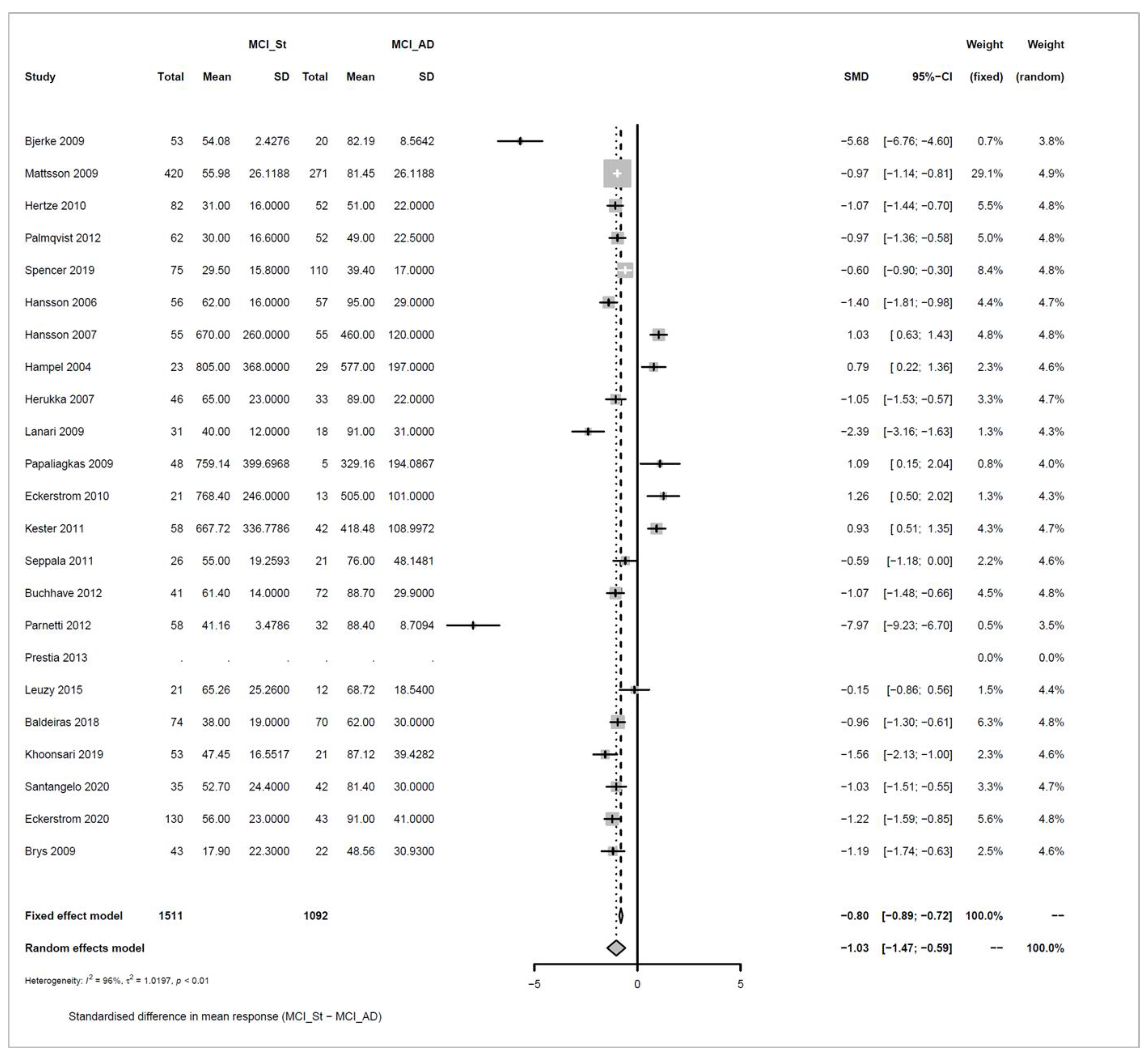
Appendix A.4. P-Tau
data <- read.csv(“sheet_Ptau_3groups.csv”, as.is=TRUE)
Appendix A.4.1. Stable MCI (MCI_St) versus MCI_AD
Models and Significance Tests for Overall Effect and Between-Study Heterogeneity
| meta <- metacont(N.MCI_St, Mean.MCI_St, SD.MCI_St, N.MCI_AD, Mean.MCI_AD, SD.MCI_AD, |
| sm=“SMD”, data=data, studlab=paste(Author, Year)) |
| ## Warning in metacont(N.MCI_St, Mean.MCI_St, SD.MCI_St, N.MCI_AD, Mean.MCI_AD,: |
| ## Note, studies with non-positive values for n.e and / or n.c get no weight in |
| ## meta-analysis. |
| meta$label.e <- “MCI_St” |
| meta$label.c <- “MCI_AD” |
| print(meta, digits=2) |
| ## SMD 95%-CI %W(fixed) %W(random) |
| ## Bjerke 2009 -5.68 [-6.76; -4.60] 0.7 3.8 |
| ## Mattsson 2009 -0.97 [-1.14; -0.81] 29.1 4.9 |
| ## Hertze 2010 -1.07 [-1.44; -0.70] 5.5 4.8 |
| ## Palmqvist 2012 -0.97 [-1.36; -0.58] 5.0 4.8 |
| ## Spencer 2019 -0.60 [-0.90; -0.30] 8.4 4.8 |
| ## Hansson 2006 -1.40 [-1.81; -0.98] 4.4 4.7 |
| ## Hansson 2007 1.03 [ 0.63; 1.43] 4.8 4.8 |
| ## Hampel 2004 0.79 [ 0.22; 1.36] 2.3 4.6 |
| ## Herukka 2007 -1.05 [-1.53; -0.57] 3.3 4.7 |
| ## Lanari 2009 -2.39 [-3.16; -1.63] 1.3 4.3 |
| ## Papaliagkas 2009 1.09 [ 0.15; 2.04] 0.8 4.0 |
| ## Eckerstrom 2010 1.26 [ 0.50; 2.02] 1.3 4.3 |
| ## Kester 2011 0.93 [ 0.51; 1.35] 4.3 4.7 |
| ## Seppala 2011 -0.59 [-1.18; 0.00] 2.2 4.6 |
| ## Buchhave 2012 -1.07 [-1.48; -0.66] 4.5 4.8 |
| ## Parnetti 2012 -7.97 [-9.23; -6.70] 0.5 3.5 |
| ## Prestia 2013 NA 0.0 0.0 |
| ## Leuzy 2015 -0.15 [-0.86; 0.56] 1.5 4.4 |
| ## Baldeiras 2018 -0.96 [-1.30; -0.61] 6.3 4.8 |
| ## Khoonsari 2019 -1.56 [-2.13; -1.00] 2.3 4.6 |
| ## Santangelo 2020 -1.03 [-1.51; -0.55] 3.3 4.7 |
| ## Eckerstrom 2020 -1.22 [-1.59; -0.85] 5.6 4.8 |
| ## Brys 2009 -1.19 [-1.74; -0.63] 2.5 4.6 |
| ## |
| ## Number of studies combined: k = 22 |
| ## Number of observations: o = 2603 |
| ## |
| ## SMD 95%-CI z p-value |
| ## Fixed effect model -0.80 [-0.89; -0.72] -18.08 < 0.0001 |
| ## Random effects model -1.03 [-1.47; -0.59] -4.56 < 0.0001 |
| ## |
| ## Quantifying heterogeneity: |
| ## tau^2 = 1.0197; tau = 1.0098; I^2 = 95.6% [94.4%; 96.6%]; H = 4.77 [4.21; 5.40] |
| ## |
| ## Test of heterogeneity: |
| ## Q d.f. p-value |
| ## 477.66 21 < 0.0001 |
| ## |
| ## Details on meta-analytical method: |
| ## - Inverse variance method |
| ## - DerSimonian-Laird estimator for tau^2 |
| ## - Hedges’ g (bias corrected standardised mean difference) |
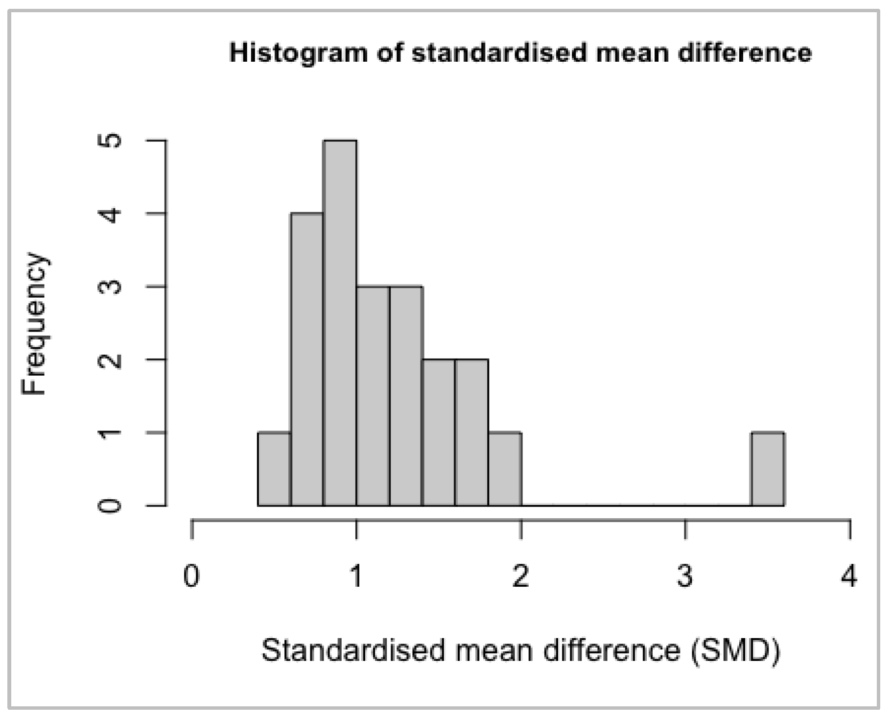
Normality Assumptions
| hist(as.numeric(meta$TE, na.rm=TRUE), xlim=c(-10,4), breaks=12, cex.main=0.9, main=“ |
| Histogram of standardised mean difference”, xlab=“Standardised mean difference (SMD) |
| ” ) |

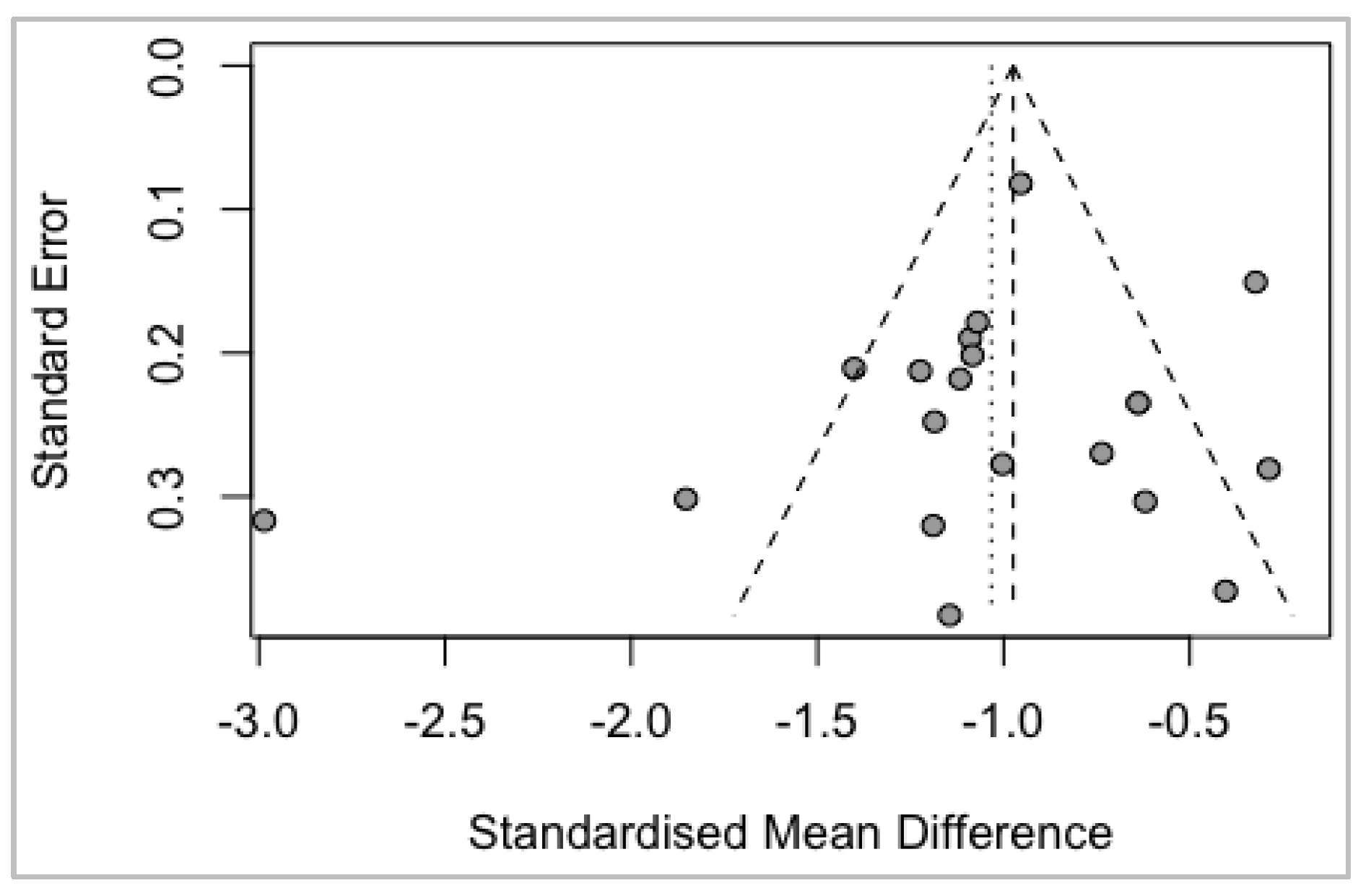
Bias Analysis
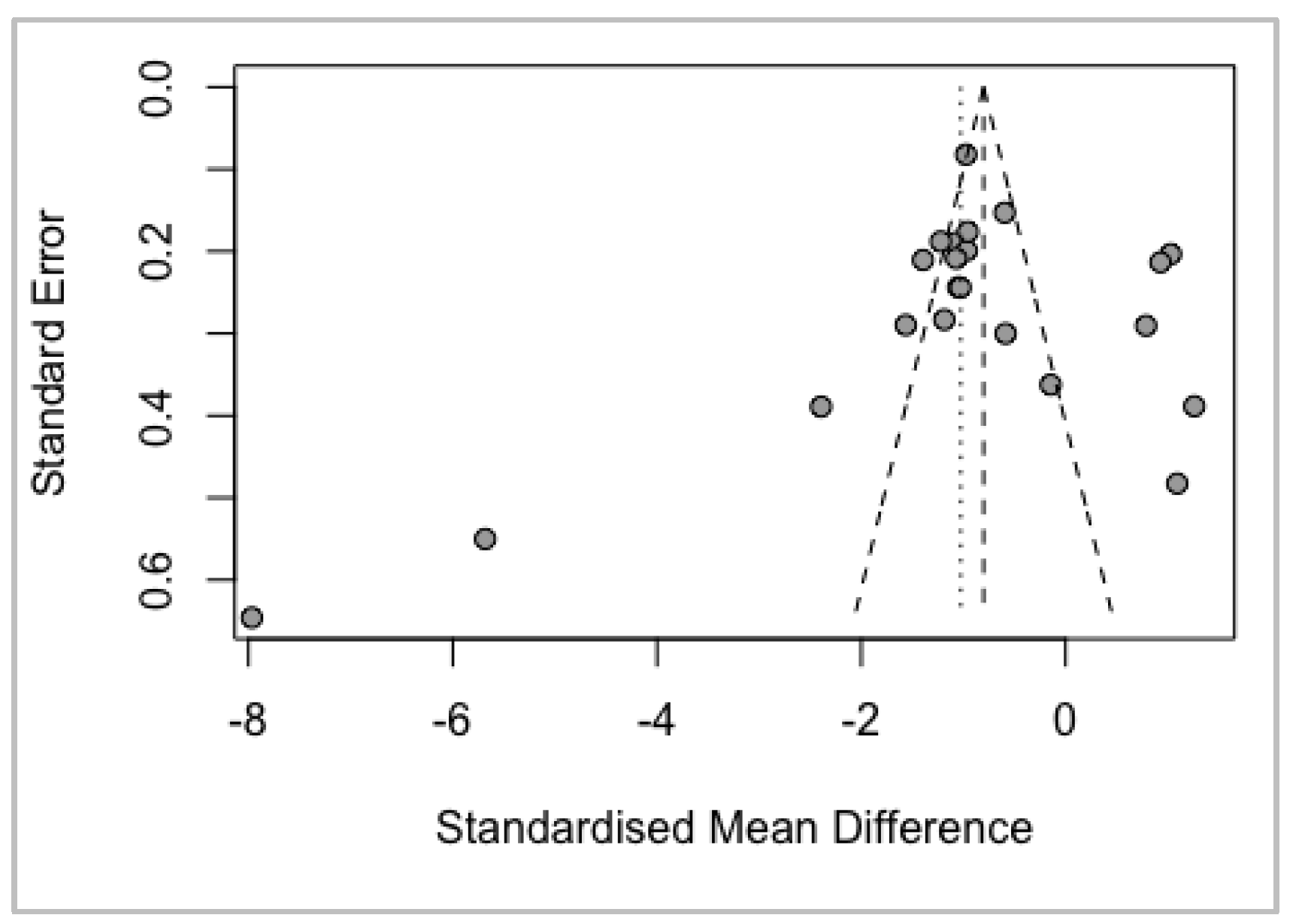
	      funnel
        (meta)

Summary Plot of the Meta-Analysis Results
| pdf(file=“forest_Ptau_MCI_StvsMCI_AD.pdf”, paper=“a4r”) |
| forest(meta, xlab=“Standardised difference in mean response (MCI_St - MCI_AD)”, |
| xlab.pos=-20, smlab.pos=-20, fontsize =5) |
| dev.off() |
Appendix A.4.2. HC vs. MCI_AD
Models and Significance Tests for Overall Effect and Between-Study Heterogeneity
| meta <- metacont(N.HC, Mean.HC, SD.HC, N.MCI_AD, Mean.MCI_AD, SD.MCI_AD, |
| sm=“SMD”, data=data, studlab=paste(Author, Year)) |
| ## Warning in metacont(N.HC, Mean.HC, SD.HC, N.MCI_AD, Mean.MCI_AD, SD.MCI_AD, : |
| ## Note, studies with non-positive values for n.e and / or n.c get no weight in |
| ## meta-analysis. |
| meta$label.e <- “HC” |
| meta$label.c <- “MCI_AD” |
| print(meta, digits=2) |
| ## SMD 95%-CI %W(fixed) %W(random) |
| ## Bjerke 2009 NA 0.0 0.0 |
| ## Mattsson 2009 -1.13 [-1.31; -0.96] 55.9 55.9 |
| ## Hertze 2010 -0.99 [-1.43; -0.55] 8.9 8.9 |
| ## Palmqvist 2012 NA 0.0 0.0 |
| ## Spencer 2019 NA 0.0 0.0 |
| ## Hansson 2006 NA 0.0 0.0 |
| ## Hansson 2007 NA 0.0 0.0 |
| ## Hampel 2004 NA 0.0 0.0 |
| ## Herukka 2007 -1.14 [-1.59; -0.68] 8.4 8.4 |
| ## Lanari 2009 NA 0.0 0.0 |
| ## Papaliagkas 2009 NA 0.0 0.0 |
| ## Eckerstrom 2010 NA 0.0 0.0 |
| ## Kester 2011 NA 0.0 0.0 |
| ## Seppala 2011 -0.47 [-1.15; 0.22] 3.7 3.7 |
| ## Buchhave 2012 -1.04 [-1.46; -0.63] 10.2 10.2 |
| ## Parnetti 2012 NA 0.0 0.0 |
| ## Prestia 2013 NA 0.0 0.0 |
| ## Leuzy 2015 NA 0.0 0.0 |
| ## Baldeiras 2018 -1.21 [-1.57; -0.84] 13.0 13.0 |
| ## Khoonsari 2019 NA 0.0 0.0 |
| ## Santangelo 2020 NA 0.0 0.0 |
| ## Eckerstrom 2020 NA 0.0 0.0 |
| ## Brys 2009 NA 0.0 0.0 |
| ## |
| ## Number of studies combined: k = 6 |
| ## Number of observations: o = 1749 |
| ## |
| ## SMD 95%-CI z p-value |
| ## Fixed effect model -1.10 [-1.23; -0.96] -16.29 < 0.0001 |
| ## Random effects model -1.10 [-1.23; -0.96] -16.29 < 0.0001 |
| ## |
| ## Quantifying heterogeneity: |
| ## tau^2 = 0; tau = 0; I^2 = 0.0% [0.0%; 74.6%]; H = 1.00 [1.00; 1.99] |
| ## |
| ## Test of heterogeneity: |
| ## Q d.f. p-value |
| ## 4.06 5 0.5414 |
| ## |
| ## Details on meta-analytical method: |
| ## - Inverse variance method |
| ## - DerSimonian-Laird estimator for tau^2 |
| ## - Hedges’ g (bias corrected standardised mean difference) |
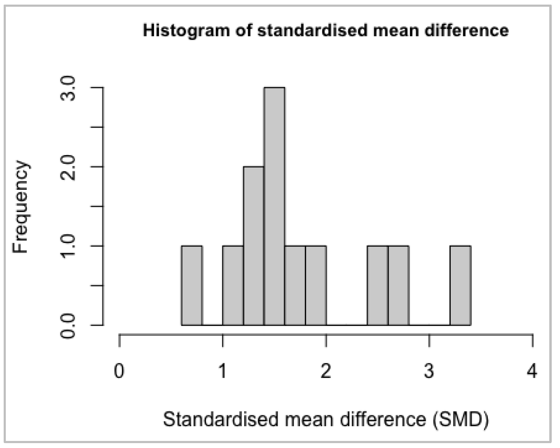
Normality Assumptions
| hist(as.numeric(meta$TE, na.rm=TRUE), xlim=c(-1.5,0), breaks=12, cex.main=0.9, main= |
| “Histogram of standardised mean difference”, xlab=“Standardised mean difference (SMD |
| )”) |

Bias Analysis
funnel(meta)

Summary Plot of the Meta-Analysis Results
| pdf(file=“forest_Ptau_HCvsMCI_AD.pdf”, paper=“a4r”) |
| forest(meta, xlab=“Standardised difference in mean response (HC - MCI_AD)”, |
| xlab.pos=-20, smlab.pos=-20, fontsize =5) |
| dev.off() |
References
- World Health Organization. Life Expectancy at Birth (Years). Available online: https://www.who.int/data/gho/data/indicators/indicator-details/GHO/life-expectancy-at-birth-(years) (accessed on 18 June 2022).
- Xia, X.; Jiang, Q.; McDermott, J.; Han, J.-D.J. Aging and Alzheimer’s disease: Comparison and associations from molecular to system level. Aging Cell 2018, 17, e12802. [Google Scholar] [CrossRef] [Green Version]
- Guerreiro, R.; Bras, J. The age factor in Alzheimer’s disease. Genome Med. 2015, 7, 106. [Google Scholar] [CrossRef] [Green Version]
- Sperling, R.A.; Karlawish, J.; Johnson, K.A. Preclinical Alzheimer disease-the challenges ahead. Nat. Rev. Neurol. 2013, 9, 54–58. [Google Scholar] [CrossRef] [Green Version]
- Bachurin, S.O.; Bovina, E.V.; Ustyugov, A.A. Drugs in Clinical Trials for Alzheimer’s Disease: The Major Trends. Med. Res. Rev. 2017, 37, 1186–1225. [Google Scholar] [CrossRef]
- Karran, E.; Hardy, J. A critique of the drug discovery and phase 3 clinical programs targeting the amyloid hypothesis for Alzheimer disease. Ann. Neurol. 2014, 76, 185–205. [Google Scholar] [CrossRef]
- Hebert, L.E.; Scherr, P.A.; Bienias, J.L.; Bennett, D.A.; Evans, D.A. Alzheimer disease in the US population: Prevalence estimates using the 2000 census. Arch. Neurol. 2003, 60, 1119–1122. [Google Scholar] [CrossRef] [Green Version]
- Hebert, L.E.; Weuve, J.; Scherr, P.A.; Evans, D.A. Alzheimer disease in the United States (2010–2050) estimated using the 2010 census. Neurology 2013, 80, 1778–1783. [Google Scholar] [CrossRef] [Green Version]
- Ritchie, C.W.; Smailagic, N.; Noel-Storr, A.; Takwoingi, Y.; Flicker, L.; Mason, S.E.; McShane, R. Plasma and cerebrospinal fluid amyloid beta for the diagnosis of Alzheimer’s disease dementia and other dementias in people with mild cognitive impairment (MCI). Cochrane Database Syst. Rev. 2014, 6, CD008782. [Google Scholar] [CrossRef]
- Vellas, B.; Andrieu, S.; Sampaio, C.; Coley, N.; Wilcock, G. Endpoints for trials in Alzheimer’s disease: A European task force consensus. Lancet. Neurol. 2008, 7, 436–450. [Google Scholar] [CrossRef]
- Peters, D.G.; Connor, J.R.; Meadowcroft, M.D. The relationship between iron dyshomeostasis and amyloidogenesis in Alzheimer’s disease: Two sides of the same coin. Neurobiol. Dis. 2015, 81, 49–65. [Google Scholar] [CrossRef] [Green Version]
- Lewczuk, P.; Riederer, P.; O’Bryant, S.E.; Verbeek, M.M.; Dubois, B.; Visser, P.J.; Jellinger, K.A.; Engelborghs, S.; Ramirez, A.; Parnetti, L.; et al. Cerebrospinal fluid and blood biomarkers for neurodegenerative dementias: An update of the Consensus of the Task Force on Biological Markers in Psychiatry of the World Federation of Societies of Biological Psychiatry. World J. Biol. Psychiatry 2018, 19, 244–328. [Google Scholar] [CrossRef] [PubMed]
- Yokomizo, J.E.; Simon, S.S.; de Campos Bottino, C.M. Cognitive screening for dementia in primary care: A systematic review. Int. Psychogeriatr. 2014, 26, 1783–1804. [Google Scholar] [CrossRef] [PubMed]
- Cullen, B.; O’Neill, B.; Evans, J.J.; Coen, R.F.; Lawlor, B.A. A review of screening tests for cognitive impairment. J. Neurol. Neurosurg Psychiatry 2007, 78, 790–799. [Google Scholar] [CrossRef] [Green Version]
- Molinuevo, J.L.; Ayton, S.; Batrla, R.; Bednar, M.M.; Bittner, T.; Cummings, J.; Fagan, A.M.; Hampel, H.; Mielke, M.M.; Mikulskis, A.; et al. Current state of Alzheimer’s fluid biomarkers. Acta Neuropathol. 2018, 136, 821–853. [Google Scholar] [CrossRef] [Green Version]
- Olsson, B.; Lautner, R.; Andreasson, U.; Öhrfelt, A.; Portelius, E.; Bjerke, M.; Hölttä, M.; Rosén, C.; Olsson, C.; Strobel, G.; et al. CSF and blood biomarkers for the diagnosis of Alzheimer’s disease: A systematic review and meta-analysis. Lancet Neurol. 2016, 15, 673–684. [Google Scholar] [CrossRef]
- Braak, H.; Del Tredici, K. The pathological process underlying Alzheimer’s disease in individuals under thirty. Acta Neuropathol. 2011, 121, 171–181. [Google Scholar] [CrossRef]
- Jack, C.R., Jr.; Knopman, D.S.; Jagust, W.J.; Petersen, R.C.; Weiner, M.W.; Aisen, P.S.; Shaw, L.M.; Vemuri, P.; Wiste, H.J.; Weigand, S.D.; et al. Tracking pathophysiological processes in Alzheimer’s disease: An updated hypothetical model of dynamic biomarkers. Lancet Neurol. 2013, 12, 207–216. [Google Scholar] [CrossRef] [Green Version]
- Mankhong, S.; Kim, S.; Lee, S.; Kwak, H.-B.; Park, D.-H.; Joa, K.-L.; Kang, J.-H. Development of Alzheimer’s Disease Biomarkers: From CSF- to Blood-Based Biomarkers. Biomedicines 2022, 10, 850. [Google Scholar] [CrossRef]
- Li, X.; Li, T.Q.; Andreasen, N.; Wiberg, M.K.; Westman, E.; Wahlund, L.O. The association between biomarkers in cerebrospinal fluid and structural changes in the brain in patients with Alzheimer’s disease. J. Intern. Med. 2014, 275, 418–427. [Google Scholar] [CrossRef] [Green Version]
- Blennow, K.; Hampel, H.; Weiner, M.; Zetterberg, H. Cerebrospinal fluid and plasma biomarkers in Alzheimer disease. Nat. Rev. Neurol. 2010, 6, 131–144. [Google Scholar] [CrossRef]
- de Souza, L.C.; Chupin, M.; Lamari, F.; Jardel, C.; Leclercq, D.; Colliot, O.; Lehéricy, S.; Dubois, B.; Sarazin, M. CSF tau markers are correlated with hippocampal volume in Alzheimer’s disease. Neurobiol. Aging 2012, 33, 1253–1257. [Google Scholar] [CrossRef] [PubMed]
- Skillbäck, T.; Farahmand, B.Y.; Rosén, C.; Mattsson, N.; Nägga, K.; Kilander, L.; Religa, D.; Wimo, A.; Winblad, B.; Schott, J.M.; et al. Cerebrospinal fluid tau and amyloid-β1-42 in patients with dementia. Brain 2015, 138, 2716–2731. [Google Scholar] [CrossRef] [PubMed] [Green Version]
- Sämgård, K.; Zetterberg, H.; Blennow, K.; Hansson, O.; Minthon, L.; Londos, E. Cerebrospinal fluid total tau as a marker of Alzheimer’s disease intensity. Int. J. Geriatr. Psychiatry 2010, 25, 403–410. [Google Scholar] [CrossRef]
- Iqbal, K.; Liu, F.; Gong, C.X.; Grundke-Iqbal, I. Tau in Alzheimer disease and related tauopathies. Curr. Alzheimer Res. 2010, 7, 656–664. [Google Scholar] [CrossRef] [Green Version]
- Seppälä, T.T.; Nerg, O.; Koivisto, A.M.; Rummukainen, J.; Puli, L.; Zetterberg, H.; Pyykkö, O.T.; Helisalmi, S.; Alafuzoff, I.; Hiltunen, M.; et al. CSF biomarkers for Alzheimer disease correlate with cortical brain biopsy findings. Neurology 2012, 78, 1568–1575. [Google Scholar] [CrossRef] [PubMed]
- Mielke, M.M.; Dage, J.L.; Frank, R.D.; Algeciras-Schimnich, A.; Knopman, D.S.; Lowe, V.J.; Bu, G.; Vemuri, P.; Graff-Radford, J.; Jack, C.R.; et al. Performance of plasma phosphorylated tau 181 and 217 in the community. Nat. Med. 2022. [Google Scholar] [CrossRef]
- Page, M.J.; McKenzie, J.E.; Bossuyt, P.M.; Boutron, I.; Hoffmann, T.C.; Mulrow, C.D.; Shamseer, L.; Tetzlaff, J.M.; Akl, E.A.; Brennan, S.E.; et al. The PRISMA 2020 statement: An updated guideline for reporting systematic reviews. BMJ 2021, 372, n71. [Google Scholar] [CrossRef] [PubMed]
- Zetterberg, H.; Wahlund, L.O.; Blennow, K. Cerebrospinal fluid markers for prediction of Alzheimer’s disease. Neurosci. Lett. 2003, 352, 67–69. [Google Scholar] [CrossRef]
- Spencer, B.E.; Jennings, R.G.; Brewer, J.B.; Alzheimer’s Disease Neuroimaging Initiative. Combined Biomarker Prognosis of Mild Cognitive Impairment: An 11-Year Follow-Up Study in the Alzheimer’s Disease Neuroimaging Initiative. J. Alzheimers Dis. 2019, 68, 1549–1559. [Google Scholar] [CrossRef]
- Cui, Y.; Liu, B.; Luo, S.; Zhen, X.; Fan, M.; Liu, T.; Zhu, W.; Park, M.; Jiang, T.; Jin, J.S. Identification of conversion from mild cognitive impairment to Alzheimer’s disease using multivariate predictors. PLoS ONE 2011, 6, e21896. [Google Scholar] [CrossRef]
- Hansson, O.; Zetterberg, H.; Buchhave, P.; Londos, E.; Blennow, K.; Minthon, L. Association between CSF biomarkers and incipient Alzheimer’s disease in patients with mild cognitive impairment: A follow-up study. Lancet Neurol. 2006, 5, 228–234. [Google Scholar] [CrossRef] [Green Version]
- Hansson, O.; Zetterberg, H.; Buchhave, P.; Andreasson, U.; Londos, E.; Minthon, L.; Blennow, K. Prediction of Alzheimer’s disease using the CSF Abeta42/Abeta40 ratio in patients with mild cognitive impairment. Dement. Geriatr. Cogn. Disord. 2007, 23, 316–320. [Google Scholar] [CrossRef] [PubMed]
- Herukka, S.-K.; Helisalmi, S.; Hallikainen, M.; Tervo, S.; Soininen, H.; Pirttilä, T. CSF Aβ42, Tau and phosphorylated Tau, APOE ɛ4 allele and MCI type in progressive MCI. Neurobiol. Aging 2007, 28, 507–514. [Google Scholar] [CrossRef] [PubMed]
- Khoonsari, P.E.; Shevchenko, G.; Herman, S.; Remnestål, J.; Giedraitis, V.; Brundin, R.; Degerman Gunnarsson, M.; Kilander, L.; Zetterberg, H.; Nilsson, P.; et al. Improved Differential Diagnosis of Alzheimer’s Disease by Integrating ELISA and Mass Spectrometry-Based Cerebrospinal Fluid Biomarkers. J. Alzheimers Dis. 2019, 67, 639–651. [Google Scholar] [CrossRef] [PubMed] [Green Version]
- Santangelo, R.; Masserini, F.; Agosta, F.; Sala, A.; Caminiti, S.P.; Cecchetti, G.; Caso, F.; Martinelli, V.; Pinto, P.; Passerini, G.; et al. CSF p-tau/Aβ(42) ratio and brain FDG-PET may reliably detect MCI “imminent” converters to AD. Eur. J. Nucl. Med. Mol. Imaging 2020, 47, 3152–3164. [Google Scholar] [CrossRef]
- Baldeiras, I.; Santana, I.; Leitão, M.J.; Gens, H.; Pascoal, R.; Tábuas-Pereira, M.; Beato-Coelho, J.; Duro, D.; Almeida, M.R.; Oliveira, C.R. Addition of the Aβ42/40 ratio to the cerebrospinal fluid biomarker profile increases the predictive value for underlying Alzheimer’s disease dementia in mild cognitive impairment. Alzheimers Res. 2018, 10, 33. [Google Scholar] [CrossRef] [Green Version]
- Luo, D.; Wan, X.; Liu, J.; Tong, T. Optimally estimating the sample mean from the sample size, median, mid-range, and/or mid-quartile range. Stat. Methods Med. Res. 2018, 27, 1785–1805. [Google Scholar] [CrossRef] [Green Version]
- Wan, X.; Wang, W.; Liu, J.; Tong, T. Estimating the sample mean and standard deviation from the sample size, median, range and/or interquartile range. BMC Med. Res. Methodol. 2014, 14, 135. [Google Scholar] [CrossRef] [Green Version]
- Petersen, R.C.; Smith, G.E.; Ivnik, R.J.; Tangalos, E.G.; Schaid, D.J.; Thibodeau, S.N.; Kokmen, E.; Waring, S.C.; Kurland, L.T. Apolipoprotein E status as a predictor of the development of Alzheimer’s disease in memory-impaired individuals. JAMA 1995, 273, 1274–1278. [Google Scholar] [CrossRef]
- Petersen, R.C.; Smith, G.E.; Waring, S.C.; Ivnik, R.J.; Tangalos, E.G.; Kokmen, E. Mild cognitive impairment: Clinical characterization and outcome. Arch. Neurol. 1999, 56, 303–308. [Google Scholar] [CrossRef]
- Petersen, R.C. Clinical practice. Mild cognitive impairment. N. Engl. J. Med. 2011, 364, 2227–2234. [Google Scholar] [CrossRef] [PubMed] [Green Version]
- Brys, M.; Pirraglia, E.; Rich, K.; Rolstad, S.; Mosconi, L.; Switalski, R.; Glodzik-Sobanska, L.; De Santi, S.; Zinkowski, R.; Mehta, P.; et al. Prediction and longitudinal study of CSF biomarkers in mild cognitive impairment. Neurobiol. Aging 2009, 30, 682–690. [Google Scholar] [CrossRef] [Green Version]
- Buchhave, P.; Minthon, L.; Zetterberg, H.; Wallin, A.K.; Blennow, K.; Hansson, O. Cerebrospinal fluid levels of β-amyloid 1-42, but not of tau, are fully changed already 5 to 10 years before the onset of Alzheimer dementia. Arch. Gen. Psychiatry 2012, 69, 98–106. [Google Scholar] [CrossRef] [PubMed]
- Bjerke, M.; Andreasson, U.; Rolstad, S.; Nordlund, A.; Lind, K.; Zetterberg, H.; Edman, A.; Blennow, K.; Wallin, A. Subcortical vascular dementia biomarker pattern in mild cognitive impairment. Dement. Geriatr. Cogn. Disord. 2009, 28, 348–356. [Google Scholar] [CrossRef] [PubMed]
- Mattsson, N.; Zetterberg, H.; Hansson, O.; Andreasen, N.; Parnetti, L.; Jonsson, M.; Herukka, S.K.; van der Flier, W.M.; Blankenstein, M.A.; Ewers, M.; et al. CSF biomarkers and incipient Alzheimer disease in patients with mild cognitive impairment. Jama 2009, 302, 385–393. [Google Scholar] [CrossRef]
- Hertze, J.; Minthon, L.; Zetterberg, H.; Vanmechelen, E.; Blennow, K.; Hansson, O. Evaluation of CSF biomarkers as predictors of Alzheimer’s disease: A clinical follow-up study of 4.7 years. J. Alzheimers Dis. 2010, 21, 1119–1128. [Google Scholar] [CrossRef] [Green Version]
- Palmqvist, S.; Hertze, J.; Minthon, L.; Wattmo, C.; Zetterberg, H.; Blennow, K.; Londos, E.; Hansson, O. Comparison of brief cognitive tests and CSF biomarkers in predicting Alzheimer’s disease in mild cognitive impairment: Six-year follow-up study. PLoS ONE 2012, 7, e38639. [Google Scholar] [CrossRef] [Green Version]
- Hampel, H.; Teipel, S.J.; Fuchsberger, T.; Andreasen, N.; Wiltfang, J.; Otto, M.; Shen, Y.; Dodel, R.; Du, Y.; Farlow, M.; et al. Value of CSF beta-amyloid1-42 and tau as predictors of Alzheimer’s disease in patients with mild cognitive impairment. Mol. Psychiatry 2004, 9, 705–710. [Google Scholar] [CrossRef] [Green Version]
- Lanari, A.; Parnetti, L. Cerebrospinal fluid biomarkers and prediction of conversion in patients with mild cognitive impairment: 4-year follow-up in a routine clinical setting. Sci. World J. 2009, 9, 961–966. [Google Scholar] [CrossRef] [Green Version]
- Papaliagkas, V.T.; Anogianakis, G.; Tsolaki, M.N.; Koliakos, G.; Kimiskidis, V.K. Progression of mild cognitive impairment to Alzheimer’s disease: Improved diagnostic value of the combined use of N200 latency and beta-amyloid(1-42) levels. Dement. Geriatr. Cogn. Disord. 2009, 28, 30–35. [Google Scholar] [CrossRef]
- Eckerström, C.; Andreasson, U.; Olsson, E.; Rolstad, S.; Blennow, K.; Zetterberg, H.; Malmgren, H.; Edman, A.; Wallin, A. Combination of hippocampal volume and cerebrospinal fluid biomarkers improves predictive value in mild cognitive impairment. Dement. Geriatr. Cogn. Disord. 2010, 29, 294–300. [Google Scholar] [CrossRef] [PubMed]
- Kester, M.I.; Verwey, N.A.; van Elk, E.J.; Blankenstein, M.A.; Scheltens, P.; van der Flier, W.M. Progression from MCI to AD: Predictive value of CSF Aβ42 is modified by APOE genotype. Neurobiol. Aging 2011, 32, 1372–1378. [Google Scholar] [CrossRef] [PubMed]
- Seppälä, T.T.; Koivisto, A.M.; Hartikainen, P.; Helisalmi, S.; Soininen, H.; Herukka, S.K. Longitudinal changes of CSF biomarkers in Alzheimer’s disease. J. Alzheimers Dis. 2011, 25, 583–594. [Google Scholar] [CrossRef] [PubMed]
- Parnetti, L.; Chiasserini, D.; Eusebi, P.; Giannandrea, D.; Bellomo, G.; De Carlo, C.; Padiglioni, C.; Mastrocola, S.; Lisetti, V.; Calabresi, P. Performance of A beta(1-40), A beta(1-42), Total Tau, and Phosphorylated Tau as Predictors of Dementia in a Cohort of Patients with Mild Cognitive Impairment. J. Alzheimers Dis. 2012, 29, 229–238. [Google Scholar] [CrossRef] [Green Version]
- Prestia, A.; Caroli, A.; van der Flier, W.M.; Ossenkoppele, R.; Van Berckel, B.; Barkhof, F.; Teunissen, C.E.; Wall, A.E.; Carter, S.F.; Schöll, M.; et al. Prediction of dementia in MCI patients based on core diagnostic markers for Alzheimer disease. Neurology 2013, 80, 1048–1056. [Google Scholar] [CrossRef] [Green Version]
- Leuzy, A.; Carter, S.F.; Chiotis, K.; Almkvist, O.; Wall, A.; Nordberg, A. Concordance and Diagnostic Accuracy of [11C]PIB PET and Cerebrospinal Fluid Biomarkers in a Sample of Patients with Mild Cognitive Impairment and Alzheimer’s Disease. J. Alzheimers Dis. 2015, 45, 1077–1088. [Google Scholar] [CrossRef] [Green Version]
- Eckerström, C.; Eckerström, M.; Göthlin, M.; Molinder, A.; Jonsson, M.; Kettunen, P.; Svensson, J.; Rolstad, S.; Wallin, A. Characteristic Biomarker and Cognitive Profile in Incipient Mixed Dementia. J. Alzheimers Dis. 2020, 73, 597–607. [Google Scholar] [CrossRef] [Green Version]
- Lewczuk, P.; Kornhuber, J.; Vanderstichele, H.; Vanmechelen, E.; Esselmann, H.; Bibl, M.; Wolf, S.; Otto, M.; Reulbach, U.; Kölsch, H.; et al. Multiplexed quantification of dementia biomarkers in the CSF of patients with early dementias and MCI: A multicenter study. Neurobiol. Aging 2008, 29, 812–818. [Google Scholar] [CrossRef]
- Shaw, L.M.; Vanderstichele, H.; Knapik-Czajka, M.; Clark, C.M.; Aisen, P.S.; Petersen, R.C.; Blennow, K.; Soares, H.; Simon, A.; Lewczuk, P.; et al. Cerebrospinal fluid biomarker signature in Alzheimer’s disease neuroimaging initiative subjects. Ann. Neurol. 2009, 65, 403–413. [Google Scholar] [CrossRef] [Green Version]
- Rosenberg, A.; Solomon, A.; Jelic, V.; Hagman, G.; Bogdanovic, N.; Kivipelto, M. Progression to dementia in memory clinic patients with mild cognitive impairment and normal β-amyloid. Alzheimers Res. 2019, 11, 99. [Google Scholar] [CrossRef] [Green Version]
- Thijssen, E.H.; La Joie, R.; Strom, A.; Fonseca, C.; Iaccarino, L.; Wolf, A.; Spina, S.; Allen, I.E.; Cobigo, Y.; Heuer, H.; et al. Plasma phosphorylated tau 217 and phosphorylated tau 181 as biomarkers in Alzheimer’s disease and frontotemporal lobar degeneration: A retrospective diagnostic performance study. Lancet Neurol. 2021, 20, 739–752. [Google Scholar] [CrossRef]
- Schwarzer, G.; Carpenter, J.; Rücker, G. Meta-Analysis with R; Springer: Berlin/Heidelberg, Germany, 2015. [Google Scholar]
- Higgins, J.P.; Thomas, J.; Chandler, J.; Cumpston, M.; Li, T.; Page, M.J.; Welch, V.A. Cochrane Handbook for Systematic Reviews of Interventions, Version 6.3 (Updated 2022). Cochrane. 2022. Available online: www.training.cochrane.org/handbook (accessed on 18 June 2022).
- Higgins, J.P.T.; Thompson, S.G.; Deeks, J.J.; Altman, D.G. Measuring inconsistency in meta-analyses. BMJ 2003, 327, 557–560. [Google Scholar] [CrossRef] [PubMed] [Green Version]
- Israel, H.; Richter, R.R. A guide to understanding meta-analysis. J. Orthop. Sports Phys. 2011, 41, 496–504. [Google Scholar] [CrossRef] [PubMed] [Green Version]


| Number of Individual Studies | Effect Size (Random Where Applicable) | Measures of Heterogeneity | Test for Heterogeneity | |||||
|---|---|---|---|---|---|---|---|---|
| SMD | p | tau2 | I2 | Q | p | |||
| Stable_MCI vs. MCI_AD | Amyloid | 22 | 1.19 | <0.0001 | 0.236 | 83.8% | 129.49 | <0.0001 |
| T-tau | 20 | −1.03 | <0.0001 | 0.167 | 79.0% | 90.45 | <0.0001 | |
| P-tau | 22 | −1.03 | <0.0001 | 1.020 | 95.6% | 477.66 | <0.0001 | |
| HC vs. MCI_AD | Amyloid | 12 | 1.73 | <0.0001 | 0.280 | 83.7% | 67.35 | <0.0001 |
| T-tau | 10 | −1.13 | <0.0001 | 0.048 | 50.5% | 18.18 | 0.0331 | |
| P-tau | 6 | −1.10 | <0.0001 | 0 | 0.0% | 4.06 | 0.5414 | |
| (a) Summary of data at early follow-up [32]. Data are given as mean (standard deviation). | |||
|---|---|---|---|
| Category (number) | Aβ1-42 (ng/L) | T-tau (ng/L) | P-tau (ng/L) |
| Non-progressive MCI (n = 56) | 551 (188) | 340 (212) | 62 (16) |
| Progressive MCI (n = 57) | 324 (101) | 816 (426) | 95 (29) |
| (b) Summary of data at late follow-up [44]. Data are given as mean (standard deviation). | |||
| Category (number) | Aβ1-42 (ng/L) | T-tau (ng/L) | P-tau (ng/L) |
| Non-progressive MCI (n = 41) | 607 (165) | 297 (182) | 61.4 (14.0) |
| Progressive MCI (n = 72) | 337 (122) | 737 (425) | 88.7 (29.9) |
| (c) Summary of patients who develop AD and other forms of dementia after being classified as non-progressive at early follow-up [29,38]. Data shown are the mean values. | |||
| Number of patients | Aβ1-42 (ng/L) | T-tau (ng/L) | P-tau (ng/L) |
| n = 15 | 397 | 490 | 63.6 |
Publisher’s Note: MDPI stays neutral with regard to jurisdictional claims in published maps and institutional affiliations. |
© 2022 by the authors. Licensee MDPI, Basel, Switzerland. This article is an open access article distributed under the terms and conditions of the Creative Commons Attribution (CC BY) license (https://creativecommons.org/licenses/by/4.0/).
Share and Cite
Ma, Y.; Brettschneider, J.; Collingwood, J.F. A Systematic Review and Meta-Analysis of Cerebrospinal Fluid Amyloid and Tau Levels Identifies Mild Cognitive Impairment Patients Progressing to Alzheimer’s Disease. Biomedicines 2022, 10, 1713. https://doi.org/10.3390/biomedicines10071713
Ma Y, Brettschneider J, Collingwood JF. A Systematic Review and Meta-Analysis of Cerebrospinal Fluid Amyloid and Tau Levels Identifies Mild Cognitive Impairment Patients Progressing to Alzheimer’s Disease. Biomedicines. 2022; 10(7):1713. https://doi.org/10.3390/biomedicines10071713
Chicago/Turabian StyleMa, Yunxing, Julia Brettschneider, and Joanna F. Collingwood. 2022. "A Systematic Review and Meta-Analysis of Cerebrospinal Fluid Amyloid and Tau Levels Identifies Mild Cognitive Impairment Patients Progressing to Alzheimer’s Disease" Biomedicines 10, no. 7: 1713. https://doi.org/10.3390/biomedicines10071713