
Machine Learning to Predict the Progression of Bone Mass Loss Associated with Personal Characteristics and a Metabolic Syndrome Scoring Index


Abstract
:1. Introduction
2. Materials and Methods
2.1. Data Source
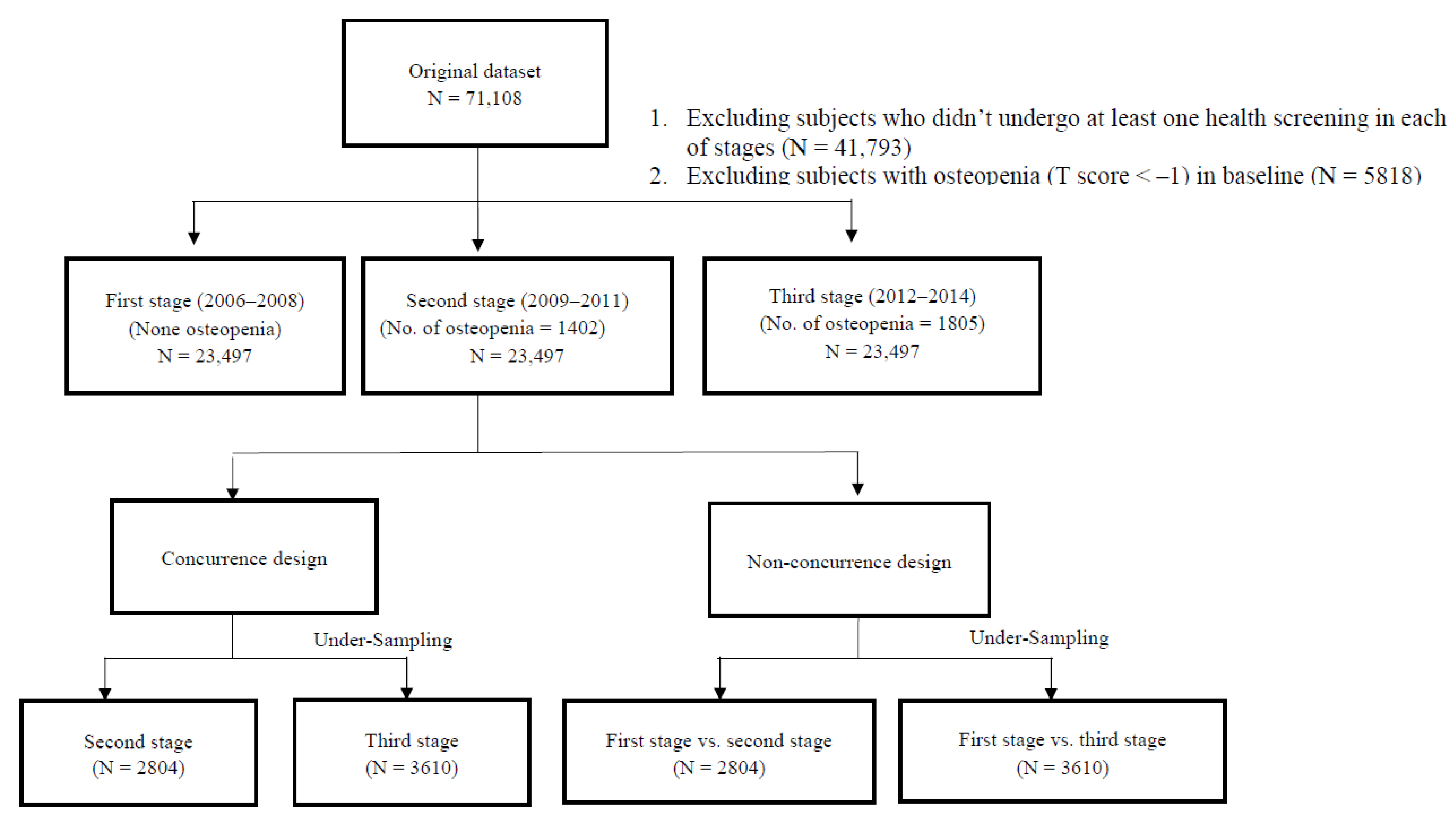
2.2. Study Sample
2.3. Response Variables
2.4. Explanatory Variables
2.5. Study Design
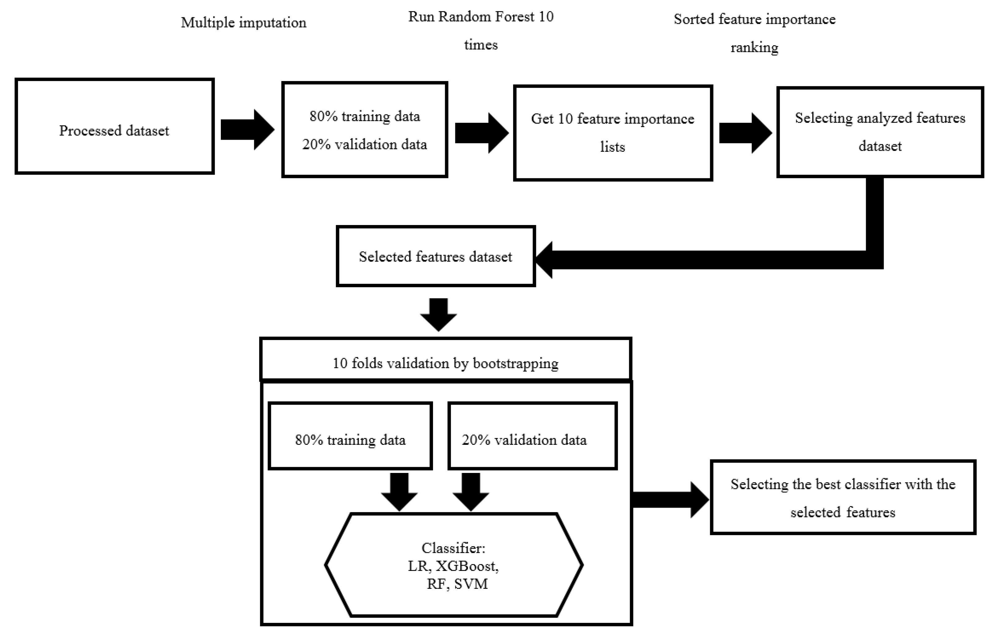
2.6. Feature Selection and Machine Learning
2.7. Model Evaluation
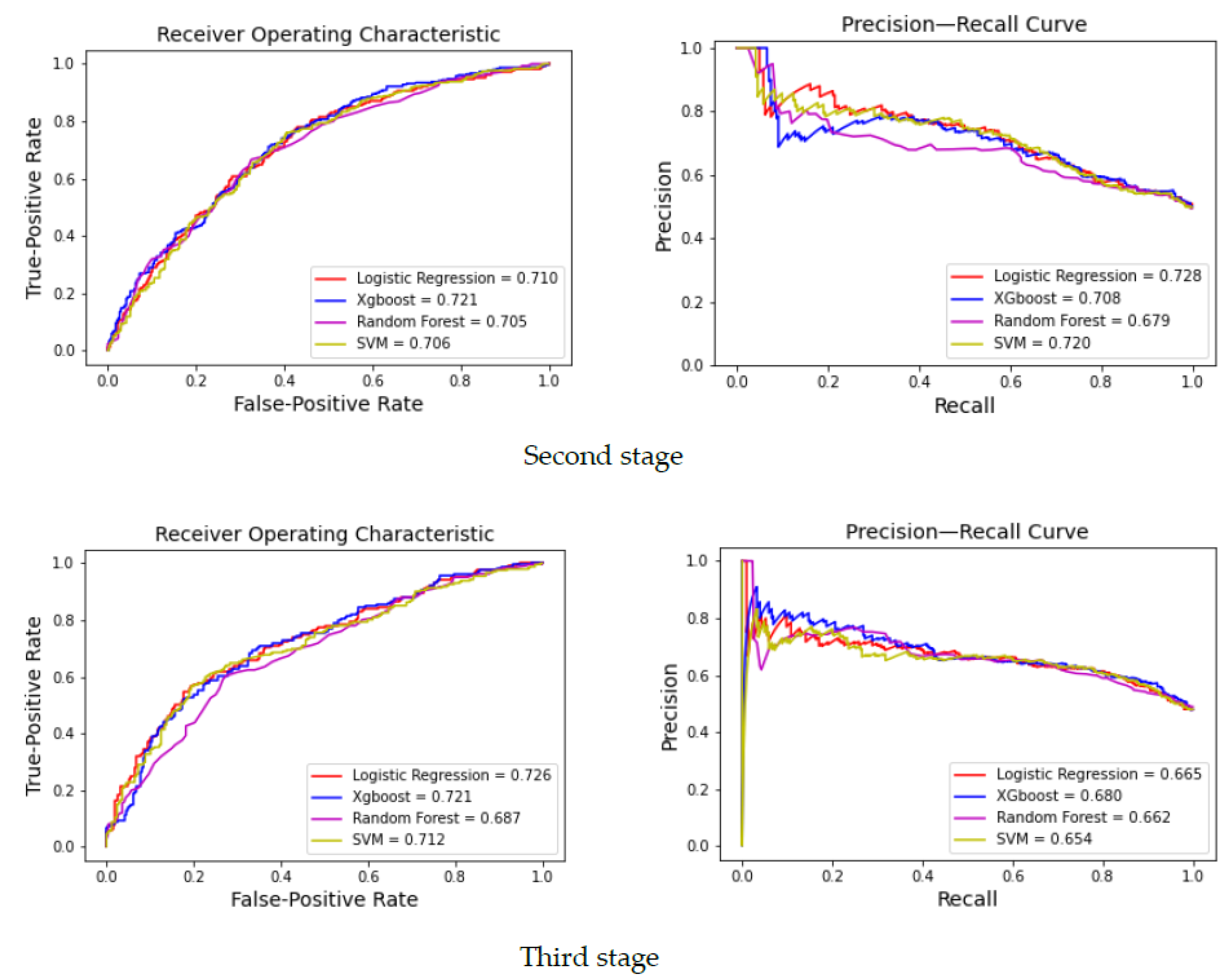
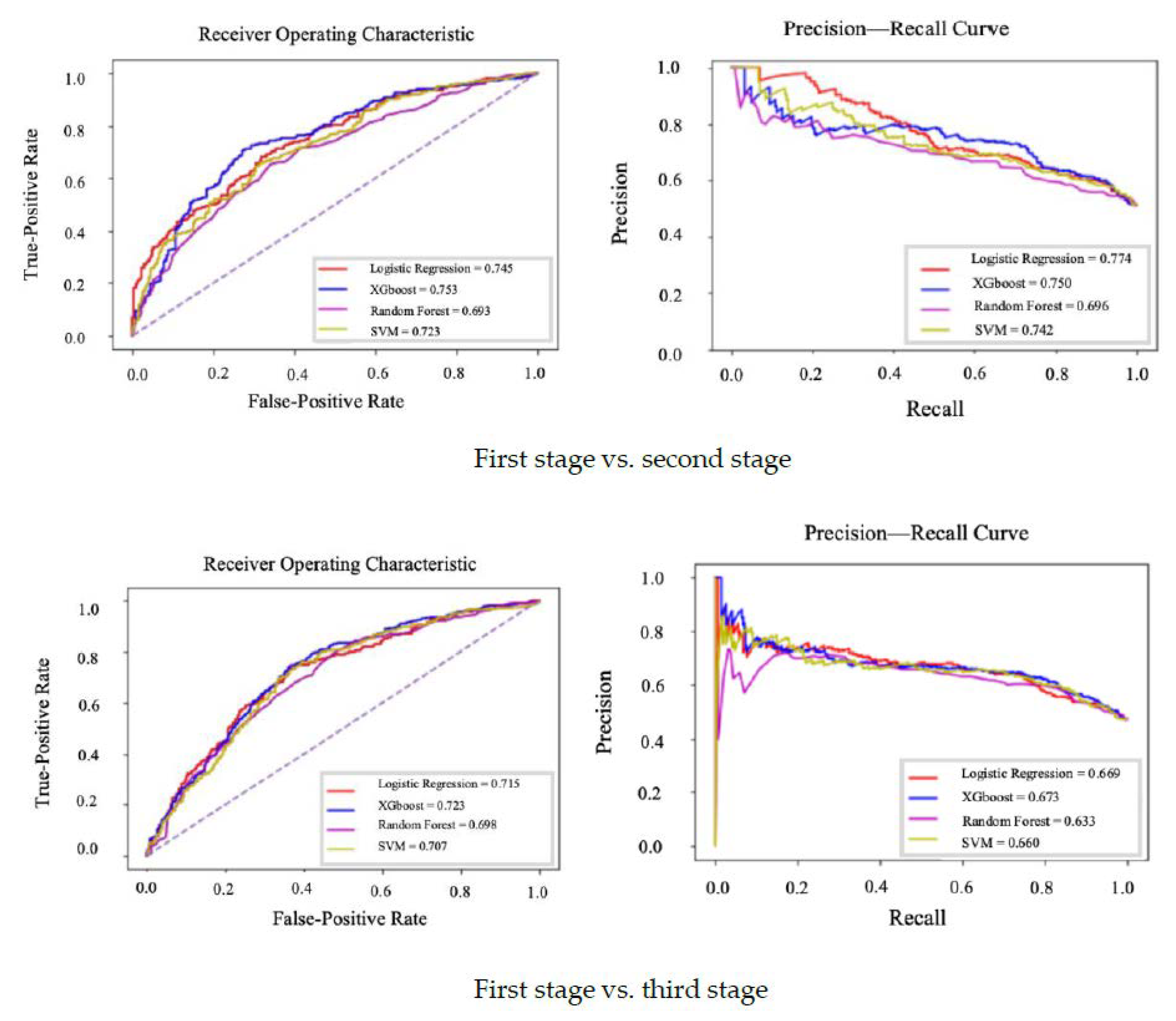
3. Results
4. Discussion
5. Conclusions
Supplementary Materials
Author Contributions
Funding
Institutional Review Board Statement
Informed Consent Statement
Data Availability Statement
Conflicts of Interest
References
- Bliuc, D.; Nguyen, N.D.; Milch, V.E.; Nguyen, T.V.; Eisman, J.A.; Center, J.R. Mortality Risk Associated with Low-Trauma Osteoporotic Fracture and Subsequent Fracture in Men and Women. JAMA J. Am. Med. Assoc. 2009, 301, 513–521. [Google Scholar] [CrossRef] [PubMed] [Green Version]
- Wright, N.C.; Looker, A.C.; Saag, K.G.; Curtis, J.R.; Delzell, E.S.; Randall, S.; Dawson-Hughes, B. The recent prevalence of osteoporosis and low bone mass in the United States based on bone mineral density at the femoral neck or lumbar spine. J. Bone Miner. Res. 2014, 29, 2520–2526. [Google Scholar] [CrossRef] [Green Version]
- Muka, T.; Trajanoska, K.; Kiefte-de Jong, J.C.; Oei1, L.; Uitterlinden, A.; Hofman, A.; Dehghan, A.; Zillikens, M.C.; Franco, O.H.; Rivadeneira, F. The Association between Metabolic Syndrome, Bone Mineral Density, Hip Bone Geometry and Fracture Risk: The Rotterdam Study. PLoS ONE 2015, 10, e0129116. [Google Scholar] [CrossRef] [PubMed]
- Clynes, M.A.; Harvey, N.C.; Curtis, E.M.; Fuggle, N.R.; Dennison, E.M.; Cooper, C. The epidemiology of osteoporosis. Br. Med. Bull. 2020, 133, 105–117. [Google Scholar] [CrossRef]
- Chen, F.P.; Huang, T.S.; Fu, T.S.; Sun, C.C.; Chao, A.S.; Tsai, T.L. Secular trends in incidence of osteoporosis in Taiwan: A nationwide population-based study. Biomed. J. 2018, 41, 314–320. [Google Scholar] [CrossRef]
- Hsu, W.L.; Chen, C.Y.; Tsauo, J.Y. Balance control in elderly people with osteoporosis. J. Formos. Med. Assoc. 2014, 113, 334–339. [Google Scholar] [CrossRef] [PubMed] [Green Version]
- Ye, C.; Xu, M.; Wang, S.; Jiang, S.; Chen, X.; Zhou, X.; He, R. Decreased Bone Mineral Density Is an Independent Predictor for the Development of Atherosclerosis: A Systematic Review and Meta-Analysis. PLoS ONE 2016, 11, e0154740. [Google Scholar] [CrossRef] [PubMed] [Green Version]
- Zhang, Y.; Feng, B. Systematic review and meta-analysis for the association of bone mineral density and osteoporosis/osteopenia with vascular calcification in women. Int. J. Rheum. Dis. 2016, 20, 154–160. [Google Scholar] [CrossRef] [PubMed]
- Rodríguez, A.J.; Scott, D.; Hodge, A.M.; English, D.R.; Giles, G.G.; Ebeling, P.R. Associations between hip bone mineral density, aortic calcification and cardiac workload in community-dwelling older Australians. Osteoporos. Int. 2017, 28, 2239–2245. [Google Scholar] [CrossRef]
- Zhang, Y.; He, B.; Wang, H.; Shi, J.; Liang, H. Associations between bone mineral density and coronary artery disease: A meta-analysis of cross-sectional studies. Arch. Osteoporos. 2020, 15, 24. [Google Scholar] [CrossRef] [PubMed]
- Almeida, M.; Han, L.; Martin-Millan, M.; Plotkin, L.I.; Stewart, S.A.; Roberson, P.K.; Kousteni, S.; O’Brien, C.A.; Bellido, T.; Parfitt, A.M.; et al. Skeletal involution by age-associated oxidative stress and its acceleration by loss of sex steroids. J. Biol. Chem. 2007, 282, 27285–27297. [Google Scholar] [CrossRef] [PubMed] [Green Version]
- Ding, C.; Parameswaran, V.; Udayan, R.; Burgess, J.; Jones, G. Circulating levels of inflammatory markers predict change in bone mineral density and resorption in older adults: A longitudinal study. J. Clin. Endocrinol. Metab. 2008, 93, 1952–1958. [Google Scholar] [CrossRef] [PubMed] [Green Version]
- Wong, S.K.; Chin, K.Y.; Suhaimi, F.H.; Ahmad, F.; Ima-Nirwana, S. The Relationship between Metabolic Syndrome and Osteoporosis: A Review. Nutrients 2016, 8, 347. [Google Scholar] [CrossRef] [PubMed] [Green Version]
- Kim, J.; Choi, Y.H. Physical activity, dietary vitamin C, and metabolic syndrome in Korean adults: The Korea National Health and Nutrition Examination Survey 2008 to 2012. Public Health 2016, 135, 30–37. [Google Scholar] [CrossRef] [PubMed]
- Liao, C.M.; Lin, C.M. Life Course Effects of Socioeconomic and Lifestyle Factors on Metabolic Syndrome and 10-Year Risk of Cardiovascular Disease: A Longitudinal Study in Taiwan Adults. Int. J. Environ. Res. Public Health. 2018, 15, 2178. [Google Scholar] [CrossRef] [Green Version]
- Yoo, S.; Cho, H.J.; Khang, Y.H. General and abdominal obesity in South Korea, 1998–2007: Gender and socioeconomic differences. Prev. Med. 2010, 51, 460–465. [Google Scholar] [CrossRef]
- Kim, J.Y.; Kim, S.H.; Cho, Y.J. Socioeconomic status in association with metabolic syndrome and coronary heart disease risk. Korean J. Fam. Med. 2013, 34, 131–138. [Google Scholar] [CrossRef] [Green Version]
- Loke, S.S.; Chang, H.W.; Li, W.C. Association between metabolic syndrome and bone mineral density in a Taiwanese elderly population. J. Bone. Miner. Metab. 2018, 36, 200–208. [Google Scholar] [CrossRef] [PubMed]
- de Cos Juez, F.J.; Suárez-Suárez, M.A.; SánchezLasheras, F.; Murcia-Mazón, A. Application of neural networks to the study of the influence of diet and lifestyle on the value of bone mineral density in postmenopausal women. Math. Comp. Model. 2011, 54, 1665–1670. [Google Scholar] [CrossRef]
- Liua, Q.; Cuia, X.; Chou, Y.C.; Abbodd, M.F.; Line, J.; Shieh, J.S. Ensemble artificial neural networks applied to predict the key risk factors of hip bone fracture for elders. Biomed. Signal. Process. Control 2015, 21, 146–156. [Google Scholar] [CrossRef] [Green Version]
- Shioji, M.; Yamamoto, T.; Ibata, T.; Tsuda, T.; Adachi, K.; Yoshimura, N. Artificial neural networks to predict future bone mineral density and bone loss rate in Japanese postmenopausal women. BMC Res. Notes 2017, 10, 590. [Google Scholar] [CrossRef] [Green Version]
- Cruz, A.S.; Lins, H.C.; Medeiros, R.V.A.; Filho, J.M.F.; da Silva, S.G. Artificial intelligence on the identification of risk groups for osteoporosis, a general review. Biomed. Eng. Online 2018, 17, 12. [Google Scholar] [CrossRef] [Green Version]
- Gurka, M.J.; Ice, C.L.; Sun, S.S.; DeBoer, M.D. A confirmatory factor analysis of the metabolic syndrome in adolescents: An examination of sex and racial/ethnic differences. Card. Diab. 2012, 11, 128. [Google Scholar] [CrossRef] [Green Version]
- Lin, C.M. An Application of Metabolic Syndrome Severity Scores in the Lifestyle Risk Assessment of Taiwanese Adults. Int. J. Environ. Res. Public Health 2020, 17, 3348. [Google Scholar] [CrossRef]
- Huang, K.C.; Lee, L.T.; Chen, C.Y.; Sung, P.K. All-cause and cardiovascular disease mortality increased with metabolic syndrome in Taiwanese. Obesity 2008, 1, 1–6. [Google Scholar] [CrossRef] [PubMed]
- Yang, X.; Tao, Q.; Sun, F.; Zhan, S. The impact of socioeconomic status on the incidence of metabolic syndrome in a Taiwanese health screening population. Int. J. Public Health 2012, 57, 551–559. [Google Scholar] [CrossRef] [PubMed]
- Looker, A.C.; Wahner, H.W.; Dunn, W.L.; Calvo, M.S.; Harris, T.B.; Heyse, S.P.; Johnston, C.C., Jr.; Lindsay, R. Updated data on proximal femur bone mineral levels of US adults. Osteoporos. Int. 1998, 8, 468–489. [Google Scholar] [CrossRef]
- Kanis, J.A.; Oden, A.; Johnell, O.; Johansson, H.; de Laet, C.; Brown, J.; Burckhardt, P.; Cooper, C.; Christiansen, C.; Cummings, S.; et al. The use of clinical risk factors enhances the performance of BMD in the prediction of hip and osteoporotic fractures in men and women. Osteoporos. Int. 2007, 18, 1033–1046. [Google Scholar] [CrossRef] [PubMed]
- Chen, J.H.; Asch, S.M. Machine Learning and Prediction in Medicine Beyond the Peak of Inflated Expectations. N. Engl. J. Med. 2017, 376, 2507–2509. [Google Scholar] [CrossRef] [PubMed] [Green Version]
- Shi, X.; Wong, Y.D.; Li, M.Z.F.; Palanisamy, C.; Chai, C. A feature learning approach based on XGBoost for driving assessment and risk prediction. Accid. Anal. Prev. 2019, 129, 170–179. [Google Scholar] [CrossRef]
- Greenwood, D. An overview of neural networks. Behav. Sci. 1991, 36, 1–33. [Google Scholar] [CrossRef] [PubMed]
- Wiener, M. Classification and Regression by randomForest. R News 2002, 2, 18–22. [Google Scholar]
- Chawla, N.V.; Bowyer, K.W.; Hall, L.O.; Kegelmeyer, W.P. SMOTE: Synthetic minority over-sampling technique. J. Artif. Intell. Res. 2002, 16, 321–357. [Google Scholar] [CrossRef]
- Friedman, J.H.; Hastie, T.; Tibshirani, R. Regularization paths for generalized linear models via coordinate descent. J. Stat. Softw. 2010, 33, 1–22. [Google Scholar] [CrossRef] [Green Version]
- Abd Elrahman, S.M.; Abraham, A. A review of class imbalance problem. J. Network Innov. Comput. 2013, 1, 332–340. [Google Scholar]
- Wu, Q.; Nasoz, F.; Jung, J.; Bhattarai, B.; Han, M.V.; Greenes, R.A.; Saag, K.G. Machine Learning Approaches for the Prediction Bone Mineral Density by using genomic and phenotypic data of 5130 older Men. Sci. Rep. 2021, 11, 4482. [Google Scholar] [CrossRef]
- Camelo, L.V.; Giatti, L.; Chor, D.; Griep, R.H.; Benseñor, I.M.; Santos, I.S.; Kawachi, I.; Barreto, S.M. Associations of life course socioeconomic position and job stress with carotid intima-media thickness. The Brazilian Longitudinal Study of Adult Health (ELSA-Brasil). Soc. Sci. Med. 2015, 141, 91–99. [Google Scholar] [CrossRef] [PubMed]
- Hoffmann, R.; Kröger, H.; Pakpahan, E. Pathways between socioeconomic status and health: Does health selection or social causation dominate in Europe? Adv. Life Course Res. 2018, 36, 23–36. [Google Scholar] [CrossRef]


| Feature | Rank | Relative Importance |
|---|---|---|
| MetS score | 1 | 1.000 |
| Body mass index | 2 | 0.959 |
| Age | 3 | 0.253 |
| Education | 4 | 0.243 |
| Sweetened beverage | 5 | 0.216 |
| Milk intake | 6 | 0.207 |
| Income | 7 | 0.194 |
| Physical activity | 8 | 0.187 |
| Sleep | 9 | 0.184 |
| Occupation | 10 | 0.162 |
| Cheese intake | 11 | 0.154 |
| Sex | 12 | 0.151 |
| Smoke | 13 | 0.133 |
| Alcohol | 14 | 0.127 |
| Vitamin C/E intake | 15 | 0.105 |
| Calcium intake | 16 | 0.103 |
| Marital status | 17 | 0.102 |
| Characteristics | Participants in 2006–2008 | Osteopenia in 2009–2011 | Osteopenia in 2012–2014 |
|---|---|---|---|
| n (%) | n (%) | n (%) | |
| Sex | |||
| Male | 13,012 (55.4) | 953 (7.3) | 1080 (8.3) |
| Female | 10,485 (44.8) | 449 (4.3) | 725 (6.9) |
| Age (yrs) | |||
| 20–39 | 11,055 (47.0) | 240 (2.9) | 176 (3.0) |
| 40–64 | 11,781 (50.1) | 1029 (7.2) | 1404 (8.7) |
| ≥65 | 661 (2.8) | 133 (14.0) | 225 (16.4) |
| Marital status | |||
| Unmarried | 5163 (23.3) | 211 (4.7) | 258 (6.5) |
| Married | 16,956 (76.7) | 1100 (6.3) | 1386 (7.8) |
| Education (yrs) | |||
| <12 | 2178 (9.4) | 289 (13.6) | 346 (16.5) |
| 12–15 | 10,529 (45.6) | 635 (6.2) | 777 (7.9) |
| ≥16 | 10,397 (45.0) | 444 (4.2) | 586 (5.5) |
| Income (NTD/yr) | |||
| <400,000 | 2676 (12.4) | 226 (9.0) | 297 (12.1) |
| 400,000–799,999 | 5797 (26.8) | 332 (6.4) | 403 (8.4) |
| >800,000 | 13,174 (60.9) | 699 (5.0) | 899 (6.4) |
| Occupation | |||
| Unemployed | 3707 (17.5) | 284 (7.5) | 422 (10.8) |
| Managed | 2562 (11.7) | 150 (5.5) | 183 (6.6) |
| Non-managed | 15,557 (71.3) | 815 (5.4) | 970 (6.6) |
| Smoke (pack/day) | |||
| None | 18,545 (82.2) | 1062 (5.6) | 1503 (7.6) |
| ≤1 | 3177 (14.1) | 181 (6.6) | 196 (7.6) |
| >1 | 839 (3.7) | 71 (10.4) | 57 (8.9) |
| Alcohol (cup/day) | |||
| None | 18,601 (83.9) | 1041 (5.7) | 1477 (7.6) |
| 1 | 1726 (7.8) | 94 (5.5) | 140 (7.6) |
| ≥2 | 1847 (8.3) | 129 (7.2) | 140 (7.8) |
| Chewing betel nut | |||
| No | 21,521 (93.8) | 1208 (5.7) | 1659 (7.6) |
| Yes | 1428 (6.2) | 93 (8.1) | 102 (8.5) |
| Physical activity (hrs/wk) | |||
| <1 | 9042 (39.6) | 503 (5.4) | 552 (6.7) |
| 1–6 | 12,805 (56.1) | 573 (6.1) | 801 (7.8) |
| ≥7 | 987 (4.3) | 126 (7.3) | 197 (10.8) |
| Sleep (hrs/day) | |||
| <6 | 4523 (20.1) | 369 (7.0) | 524 (8.9) |
| 6 | 16,467 (73.2) | 676 (5.9) | 845 (7.3) |
| ≥7 | 1506 (6.7) | 312 (5.1) | 388 (6.9) |
| Vegetarian diet | |||
| Yes | 592 (2.5) | 56 (8.2) | 271 (7.9) |
| No | 22,774 (97.5) | 1330 (5.9) | 1534 (7.6) |
| Sweetened beverage (cup/wk) | |||
| None | 7148 (30.8) | 707 (7.2) | 996 (8.8) |
| 1–6 | 10,981 (47.3) | 483 (5.0) | 560 (6.4) |
| ≥7 | 5067 (21.8) | 176 (4.9) | 189 (6.5) |
| Milk intake (cup/wk) | |||
| None | 11,545 (49.9) | 701 (6.0) | 871 (7.6) |
| 1–6 | 9491 (41.0) | 505 (5.6) | 679 (7.2) |
| ≥7 | 2093 (9.0) | 158 (7.4) | 187 (9.3) |
| Cheese intake (slice/wk) | |||
| None | 13,276 (57.5) | 824 (6.3) | 1119 (8.4) |
| 1–6 | 9390 (40.7) | 503 (5.3) | 581 (6.4) |
| ≥7 | 430 (1.9) | 33 (6.3) | 32 (6.9) |
| Vitamin C, E intake | |||
| Yes | 4180 (17.8) | 175 (4.8) | 271 (7.9) |
| No | 19,312 (82.2) | 1227 (6.2) | 1534 (7.6) |
| Calcium intake | |||
| Yes | 3990 (17.0) | 326 (8.6) | 403 (12.0) |
| No | 19,502 (93.0) | 1076 (5.5) | 1402 (7.0) |
| Hypertension medicine | |||
| Yes | 1399 (6.0) | 138 (7.1) | 226 (9.3) |
| No | 22,093 (94.0) | 1264 (5.9) | 1579 (7.5) |
| Diabetes medicine | |||
| Yes | 440 (1.9) | 47 (7.1) | 72 (8.5) |
| No | 23,052 (98.1) | 1355 (5.9) | 1733 (7.7) |
| Thyroid medicine | |||
| Yes | 252 (1.1) | 21 (6.5) | 27 (7.3) |
| No | 23,240 (98.9) | 1381 (6.0) | 1778 (7.7) |
| Lipidemia medicine | |||
| Yes | 400 (1.7) | 35 (5.7) | 68 (8.1) |
| No | 23,092 (98.3) | 1367 (6.0) | 1737 (7.7) |
| Hormone medicine | |||
| Yes | 272 (1.2) | 18 (7.9) | 15 (7.1) |
| No | 23,220 (98.8) | 1384 (5.9) | 1790 (7.7) |
| Body mass index (sd) | 23.25 (3.41) | 22.79 (3.09) | 22.85 (3.07) |
| MetS score (sd) | 0.09 (1.02) | −0.22 (0.99) | −0.22 (0.94) |
| Logistic Regression | XGBoost | Random Forest | SVM | |||||
|---|---|---|---|---|---|---|---|---|
| Non-Concurrent | Concurrent | Non-Concurrent | Concurrent | Non-Concurrent | Concurrent | Non-Concurrent | Concurrent | |
| Sensitivity | 0.682 | 0.684 | 0.733 | 0.678 | 0.663 | 0.636 | 0.736 | 0.702 |
| Specificity | 0.648 | 0.681 | 0.689 | 0.672 | 0.623 | 0.636 | 0.575 | 0.632 |
| Accuracy | 0.665 | 0.683 | 0.711 | 0.675 | 0.643 | 0.636 | 0.658 | 0.667 |
| Precision | 0.655 | 0.694 | 0.713 | 0.694 | 0.650 | 0.631 | 0.646 | 0.651 |
| ROC | 0.726 | 0.745 | 0.753 | 0.721 | 0.693 | 0.687 | 0.723 | 0.712 |
| PRC | 0.728 | 0.774 | 0.750 | 0.708 | 0.696 | 0.697 | 0.742 | 0.720 |
| F1 | 0.668 | 0.689 | 0.723 | 0.686 | 0.656 | 0.633 | 0.688 | 0.676 |
| Logistic Regression | XGBoost | Random Forest | SVM | |||||
|---|---|---|---|---|---|---|---|---|
| Non-Concurrent | Concurrent | Non-Concurrent | Concurrent | Non-Concurrent | Concurrent | Non-Concurrent | Concurrent | |
| Sensitivity | 0.704 | 0.698 | 0.745 | 0.662 | 0.680 | 0.672 | 0.751 | 0.698 |
| Specificity | 0.646 | 0.620 | 0.633 | 0.657 | 0.622 | 0.660 | 0.600 | 0.627 |
| Accuracy | 0.673 | 0.657 | 0.686 | 0.659 | 0.650 | 0.666 | 0.669 | 0.661 |
| Precision | 0.640 | 0.628 | 0.645 | 0.639 | 0.617 | 0.645 | 0.624 | 0.632 |
| ROC | 0.715 | 0.710 | 0.723 | 0.721 | 0.698 | 0.705 | 0.707 | 0.706 |
| PRC | 0.669 | 0.665 | 0.673 | 0.680 | 0.633 | 0.662 | 0.660 | 0.654 |
| F1 | 0.670 | 0.661 | 0.691 | 0.650 | 0.647 | 0.658 | 0.681 | 0.663 |
Publisher’s Note: MDPI stays neutral with regard to jurisdictional claims in published maps and institutional affiliations. |
© 2021 by the authors. Licensee MDPI, Basel, Switzerland. This article is an open access article distributed under the terms and conditions of the Creative Commons Attribution (CC BY) license (https://creativecommons.org/licenses/by/4.0/).
Share and Cite
Cheng, C.-H.; Lin, C.-Y.; Cho, T.-H.; Lin, C.-M. Machine Learning to Predict the Progression of Bone Mass Loss Associated with Personal Characteristics and a Metabolic Syndrome Scoring Index. Healthcare 2021, 9, 948. https://doi.org/10.3390/healthcare9080948
Cheng C-H, Lin C-Y, Cho T-H, Lin C-M. Machine Learning to Predict the Progression of Bone Mass Loss Associated with Personal Characteristics and a Metabolic Syndrome Scoring Index. Healthcare. 2021; 9(8):948. https://doi.org/10.3390/healthcare9080948
Chicago/Turabian StyleCheng, Chao-Hsin, Ching-Yuan Lin, Tsung-Hsun Cho, and Chih-Ming Lin. 2021. "Machine Learning to Predict the Progression of Bone Mass Loss Associated with Personal Characteristics and a Metabolic Syndrome Scoring Index" Healthcare 9, no. 8: 948. https://doi.org/10.3390/healthcare9080948