
The Application of Projection Word Embeddings on Medical Records Scoring System

 , and
, and
Abstract
:
1. Introduction
2. Method
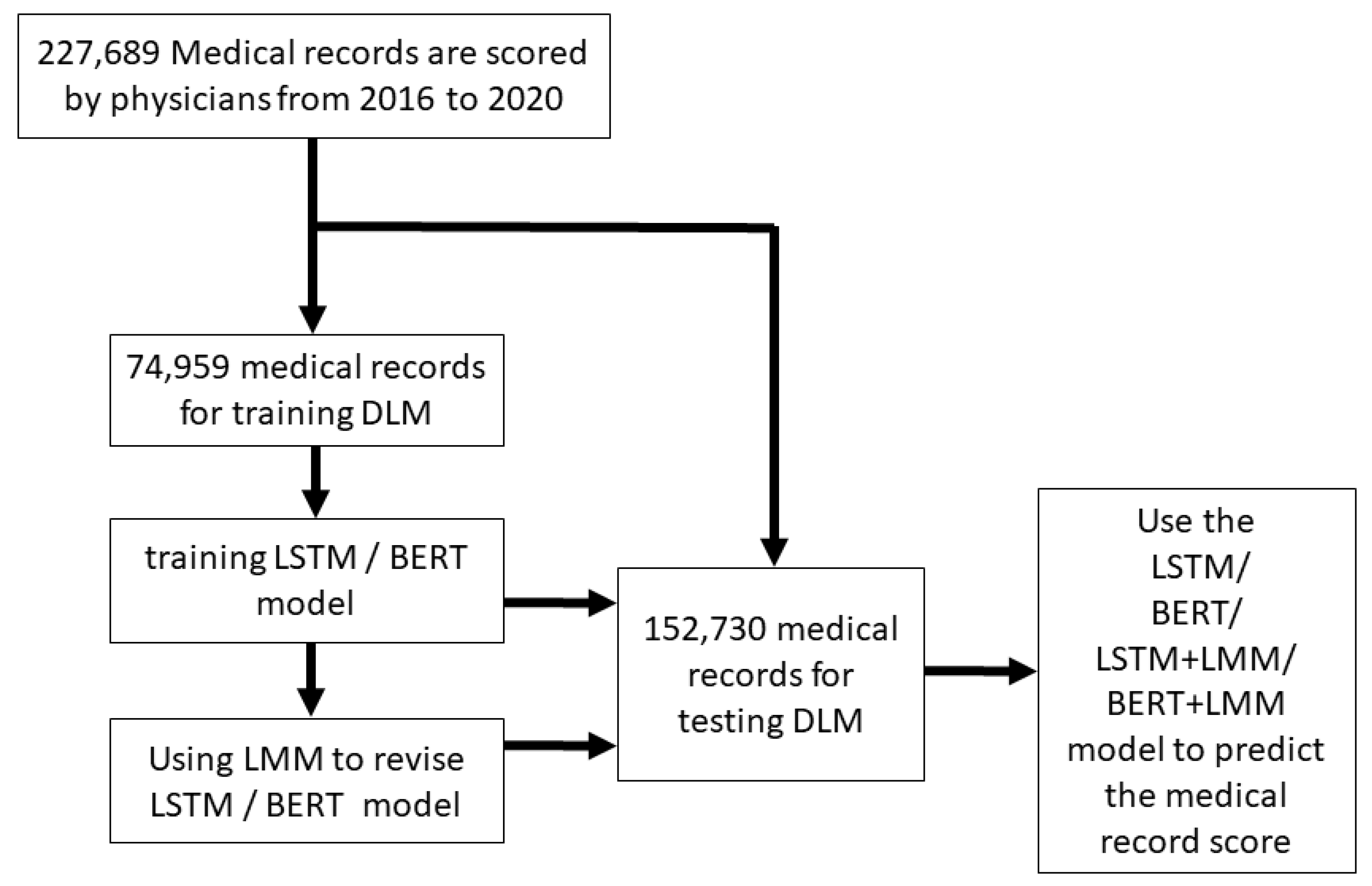
2.1. Data Source
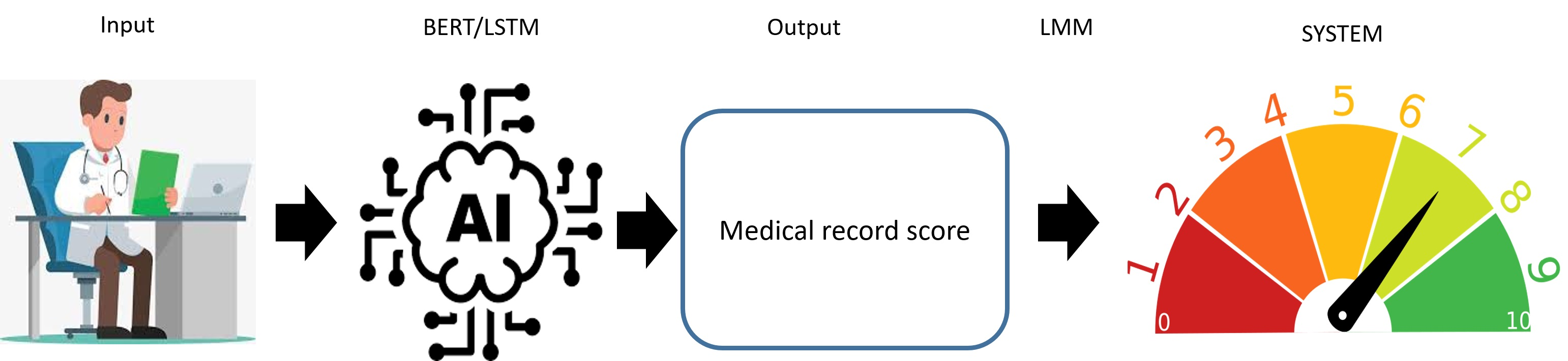
2.2. AI Algorithm
2.2.1. Long Short-Term Memory (LSTM)
2.2.2. Bidirectional Encoder Representation from Transformers (BERT)
2.3. Linear Mixed Model Function for Medical Records Scoring Prediction
2.4. Evaluation Criteria
3. Results
4. Discussion
Author Contributions
Funding
Institutional Review Board Statement
Informed Consent Statement
Data Availability Statement
Acknowledgments
Conflicts of Interest
References
- Hilbert, M.; Lopez, P. The world’s technological capacity to store, communicate, and compute information. Science 2011, 332, 60–65. [Google Scholar] [CrossRef] [Green Version]
- McAfee, A.; Brynjolfsson, E. Big data: The management revolution. Harv. Bus. Rev. 2012, 90, 60–68. [Google Scholar]
- Unstructured Data and the 80 Percent Rule; Clarabridge Bridgepoints: Reston, VA, USA, 2008; Volume Q3.
- Jeong, S.R.; Ghani, I. Semantic Computing for Big Data: Approaches, Tools, and Emerging Directions (2011–2014). TIIS 2014, 8, 2022–2042. [Google Scholar]
- Cox, M.; Ellsworth, D. Application-controlled demand paging for out-of-core visualization. In Proceedings of the 8th Conference on Visualization’97, Phoenix, AZ, USA, 24 October 1997. [Google Scholar]
- McDonald, C.J. Medical heuristics: The silent adjudicators of clinical practice. Ann. Intern. Med. 1996, 124, 56–62. [Google Scholar] [CrossRef]
- National Academies of Sciences E, Medicine. Improving Diagnosis in Health Care; National Academies Press: Washington, DC, USA, 2016. [Google Scholar]
- El-Kareh, R.; Hasan, O.; Schiff, G.D. Use of health information technology to reduce diagnostic errors. BMJ Qual. Saf. 2013, 22 (Suppl 2), ii40–ii51. [Google Scholar] [CrossRef] [Green Version]
- Murdoch, T.B.; Detsky, A.S. The inevitable application of big data to health care. JAMA 2013, 309, 1351–1352. [Google Scholar] [CrossRef]
- Spasic, I.; Livsey, J.; Keane, J.A.; Nenadic, G. Text mining of cancer-related information: Review of current status and future directions. Int. J. Med. Inform. 2014, 83, 605–623. [Google Scholar] [CrossRef]
- Cahan, A.; Cimino, J.J. A Learning Health Care System Using Computer-Aided Diagnosis. J. Med. Internet 2017, 19, e54. [Google Scholar] [CrossRef]
- Krizhevsky, A.; Sutskever, I.; Hinton, G.E. Imagenet classification with deep convolutional neural networks. Adv. Neural Inf. Process. Syst. 2012, 25, 1097–1105. [Google Scholar] [CrossRef]
- Simonyan, K.; Zisserman, A. Very deep convolutional networks for large-scale image recognition. arXiv 2014, arXiv:1409.1556. [Google Scholar]
- Szegedy, C.; Liu, W.; Jia, Y.; Sermanet, P.; Reed, S.; Anguelov, D.; Erhan, D.; Vanhoucke, V.; Rabinovich, A. Going deeper with convolutions. In Proceedings of the IEEE Conference on Computer Vision and Pattern Recognition, Boston, MA, USA, 7–12 June 2015. [Google Scholar]
- He, K.; Zhang, X.; Ren, S.; Sun, J. Deep residual learning for image recognition. In Proceedings of the IEEE Conference on Computer Vision and Pattern Recognition, Las Vegas, NV, USA, 27–30 June 2016. [Google Scholar]
- Huang, G.; Liu, Z.; Weinberger, K.Q.; van der Maaten, L. Densely connected convolutional networks. In Proceedings of the IEEE Conference on Computer Vision and Pattern Recognition, Honolulu, HI, USA, 21–26 July 2017. [Google Scholar]
- Bejnordi, B.E.; Veta, M.; van Diest, P.J.; van Ginneken, B.; Karssemeijer, N.; Litjens, G.; van der Laak, J.A.W.M.; the CAMELYON16 Consortium. Diagnostic Assessment of Deep Learning Algorithms for Detection of Lymph Node Metastases in Women with Breast Cancer. JAMA 2017, 318, 2199–2210. [Google Scholar] [CrossRef]
- Gulshan, V.; Peng, L.; Coram, M.; Stumpe, M.C.; Wu, D.; Narayanaswamy, A.; Venugopalan, S.; Widner, K.; Madams, T.; Cuadros, J.; et al. Development and Validation of a Deep Learning Algorithm for Detection of Diabetic Retinopathy in Retinal Fundus Photographs. JAMA 2016, 316, 2402–2410. [Google Scholar] [CrossRef]
- Esteva, A.; Kuprel, B.; Novoa, R.A.; Ko, J.; Swetter, S.M.; Blau, H.M.; Thrun, S. Dermatologist-level classification of skin cancer with deep neural networks. Nature 2017, 542, 115–118. [Google Scholar] [CrossRef]
- Rajpurkar, P.; Irvin, J.; Zhu, K.; Yang, B.; Mehta, H.; Duan, T.; Ding, D.; Bagul, A.; Langlotz, C.; Shpanskaya, K.; et al. CheXNet: Radiologist-Level Pneumonia Detection on Chest X-Rays with Deep Learning. arXiv 2017, arXiv:1711.05225. [Google Scholar]
- Grewal, M.; Srivastava, M.M.; Kumar, P.; Varadarajan, S. RADNET: Radiologist Level Accuracy using Deep Learning for HEMORRHAGE detection in CT Scans. arXiv 2017, arXiv:1710.04934. [Google Scholar]
- Litjens, G.; Kooi, T.; Bejnordi, B.E.; Setio AA, A.; Ciompi, F.; Ghafoorian, M.; van der Laak, J.A.W.M.; Ginneken, B.; Sánchez, C.I. A survey on deep learning in medical image analysis. Med. Image Anal. 2017, 42, 60–88. [Google Scholar] [CrossRef] [Green Version]
- Xiong, W.; Droppo, J.; Huang, X.; Seide, F.; Seltzer, M.; Stolcke, A.; Yu, D.; Zweig, G. Achieving human parity in conversational speech recognition. arXiv 2016, arXiv:1610.05256. [Google Scholar]
- Amodei, D.; Ananthanarayanan, S.; Anubhai, R.; Bai, J.; Battenberg, E.; Case, C.; Casper, J.; Catanzaro, B.; Cheng, Q.; Chen, G.; et al. Deep speech 2: End-to-end speech recognition in english and mandarin. In Proceedings of the International Conference on Machine Learning, New York, NY, USA, 20–22 June 2016. [Google Scholar]
- Dembek, Z.F.; Kortepeter, M.G.; Pavlin, J.A. Discernment between deliberate and natural infectious disease outbreaks. Epidemiol. Infect. 2007, 135, 353–371. [Google Scholar] [CrossRef]
- Tsui, F.C.; Espino, J.U.; Dato, V.M.; Gesteland, P.H.; Hutman, J.; Wagner, M.M. Technical description of RODS: A real-time public health surveillance system. J. Am. Med. Inform. Assoc. JAMIA 2003, 10, 399–408. [Google Scholar] [CrossRef] [Green Version]
- Koopman, B.; Zuccon, G.; Nguyen, A.; Bergheim, A.; Grayson, N. Automatic ICD-10 classification of cancers from free-text death certificates. Int. J. Med. Inform. 2015, 84, 956–965. [Google Scholar] [CrossRef] [Green Version]
- Koopman, B.; Karimi, S.; Nguyen, A.; McGuire, R.; Muscatello, D.; Kemp, M.; Truran, D.; Zhang, M.; Thackway, S. Automatic classification of diseases from free-text death certificates for real-time surveillance. BMC Med. Inform. Decis. Mak. 2015, 15, 53. [Google Scholar] [CrossRef] [PubMed] [Green Version]
- Koopman, B.; Zuccon, G.; Wagholikar, A.; Chu, K.; O’Dwyer, J.; Nguyen, A.; Keijzers, G. Automated Reconciliation of Radiology Reports and Discharge Summaries. In AMIA Annual Symposium Proceedings; American Medical Informatics Association: Bethesda, MD, USA, 2015; Volume 2015, pp. 775–784. [Google Scholar]
- Khachidze, M.; Tsintsadze, M.; Archuadze, M. Natural Language Processing Based Instrument for Classification of Free Text Medical Records. BioMed Res. Int. 2016, 2016, 8313454. [Google Scholar] [CrossRef] [PubMed] [Green Version]
- Mujtaba, G.; Shuib, L.; Raj, R.G.; Rajandram, R.; Shaikh, K.; Al-Garadi, M.A. Automatic ICD-10 multi-class classification of cause of death from plaintext autopsy reports through expert-driven feature selection. PLoS ONE 2017, 12, e0170242. [Google Scholar] [CrossRef] [PubMed]
- Bengio, Y.; Ducharme, R.; Vincent, P.; Jauvin, C. A neural probabilistic language model. J. Mach. Learn. Res. 2003, 3, 1137–1155. [Google Scholar]
- Yih, W.T.; Toutanova, K.; Platt, J.C.; Meek, C. Learning discriminative projections for text similarity measures. In Proceedings of the Fifteenth Conference on Computational Natural Language Learning, Portland, OR, USA, 23 June 2011. [Google Scholar]
- Mikolov, T.; Sutskever, I.; Chen, K.; Corrado, G.S.; Dean, J. Distributed representations of words and phrases and their compositionality. In Proceedings of the Advances in Neural Information Processing Systems, Lake Tahoe, Nevada, 5–10 December 2013. [Google Scholar]
- Arora, S.; Liang, Y.; Ma, T. A Simple but Tough-to-Beat Baseline for Sentence Embeddings. 2016. Available online: https://openreview.net/forum?id=SyK00v5xx (accessed on 27 September 2021).
- LeCun, Y.; Bottou, L.; Bengio, Y.; Haffner, P. Gradient-based learning applied to document recognition. Proc. IEEE. 1998, 86, 2278–2324. [Google Scholar] [CrossRef] [Green Version]
- Yih, W.T.; He, X.; Meek, C. Semantic Parsing for Single-Relation Question Answering. In Proceedings of the 52nd Annual Meeting of the Association for Computational Linguistics (Volume 2: Short Papers), Baltimore, MD, USA, 22–27 June 2014. [Google Scholar]
- Shen, Y.; He, X.; Gao, J.; Deng, L.; Mesnil, G. Learning semantic representations using convolutional neural networks for web search. In Proceedings of the 23rd International Conference on World Wide Web, Seoul, Korea, 7–11 April 2014. [Google Scholar]
- Kim, Y. Convolutional neural networks for sentence classification. arXiv 2014, arXiv:1408.5882. [Google Scholar]
- Devlin, J.; Chang, M.-W.; Lee, K.; Toutanova, K. Bert: Pre-training of deep bidirectional transformers for language understanding. arXiv 2018, arXiv:1810.04805. [Google Scholar]
- Lin, C.; Hsu, C.J.; Lou, Y.S.; Yeh, S.J.; Lee, C.C.; Su, S.L.; Chen, H.C. Artificial Intelligence Learning Semantics via External Resources for Classifying Diagnosis Codes in Discharge Notes. J. Med. Internet Res. 2017, 19, e380. [Google Scholar] [CrossRef] [Green Version]
- Choi, Y.; Chiu, C.Y.; Sontag, D. Learning Low-Dimensional Representations of Medical Concepts. AMIA Jt. Summits Transl. Sci. Proceedings. AMIA Jt. Summits Transl. Sci. 2016, 2016, 41–50. [Google Scholar]
- Wang, Y.; Liu, S.; Afzal, N.; Rastegar-Mojarad, M.; Wang, L.; Shen, F.; Kingsbury, P.; Liu, H. A comparison of word embeddings for the biomedical natural language processing. J. Biomed. Inform. 2018, 87, 12–20. [Google Scholar]
- Pakhomov, S.V.; Finley, G.; McEwan, R.; Wang, Y.; Melton, G.B. Corpus domain effects on distributional semantic modeling of medical terms. Bioinformatics 2016, 32, 3635–3644. [Google Scholar] [CrossRef] [Green Version]
- Lin, C.; Lou, Y.S.; Tsai, D.J.; Lee, C.C.; Hsu, C.J.; Wu, D.C.; Wang, M.C.; Fang, W.H. Projection Word Embedding Model With Hybrid Sampling Training for Classifying ICD-10-CM Codes: Longitudinal Observational Study. JMIR Med. Inform. 2019, 7, e14499. [Google Scholar] [CrossRef] [PubMed]
- Hochreiter, S.; Schmidhuber, J. Long Short-term Memory. Neural Comput. 1997, 9, 1735–1780. [Google Scholar] [CrossRef] [PubMed]
- Gao, Z.; Feng, A.; Song, X.; Wu, X. Target-dependent sentiment classification with BERT. IEEE Access 2019, 7, 154290–154299. [Google Scholar] [CrossRef]
- Robinson, G.K. That BLUP is a good thing: The estimation of random effects. Stat. Sci. 1991, 15–32. [Google Scholar] [CrossRef]
- Hulme, O.L.; Khurshid, S.; Weng, L.C.; Anderson, C.D.; Wang, E.Y.; Ashburner, J.M.; Ko, D.; McManus, D.D.; Benjamin, E.J.; Ellinor, P.T.; et al. Development and Validation of a Prediction Model for Atrial Fibrillation Using Electronic Health Records. JACC. Clin. Electrophysiol. 2019, 5, 1331–1341. [Google Scholar] [CrossRef] [PubMed]
- Du, Z.; Yang, Y. Accurate Prediction of Coronary Heart Disease for Patients with Hypertension from Electronic Health Records with Big Data and Machine-Learning Methods: Model Development and Performance Evaluation. JMIR Med. Inform. 2020, 8, e17257. [Google Scholar] [CrossRef] [PubMed]
- Ye, C.; Li, J.; Hao, S.; Liu, M.; Jin, H.; Zheng, L.; Xia, M.; Jin, B.; Zhu, C.; Alfreds, S.T.; et al. Identification of elders at higher risk for fall with statewide electronic health records and a machine learning algorithm. Int. J. Med. Inform. 2020, 137, 104105. [Google Scholar] [CrossRef]
- Ahuja, Y.; Kim, N.; Liang, L.; Cai, T.; Dahal, K.; Seyok, T.; Lin, C.; Finan, S.; Liao, K.; Savovoa, G.; et al. Leveraging electronic health records data to predict multiple sclerosis disease activity. Ann. Clin. Transl. Neurol. 2021, 8, 800–810. [Google Scholar] [CrossRef]
- Weegar, R.; Sundström, K. Using machine learning for predicting cervical cancer from Swedish electronic health records by mining hierarchical representations. PLoS ONE. 2020, 15, e0237911. [Google Scholar] [CrossRef]
- Manolio, T.A.; Collins, F.S.; Cox, N.J.; Goldstein, D.B.; Hindorff, L.A.; Hunter, D.J.; McCarthy, M.I.; Ramos, E.M.; Cardon, L.R.; Chakravarti, A.; et al. Finding the missing heritability of complex diseases. Nature 2009, 461, 747–753. [Google Scholar] [CrossRef] [PubMed] [Green Version]
- Lo, A.; Chernoff, H.; Zheng, T.; Lo, S.-H. Why significant variables aren’t automatically good predictors. Proc. Natl. Acad. Sci. USA 2015, 112, 13892–13897. [Google Scholar] [CrossRef] [PubMed] [Green Version]
- Visscher, P.M.; Wray, N.R.; Zhang, Q.; Sklar, P.; McCarthy, M.I.; Brown, M.A.; Yang, J. 10 years of GWAS discovery: Biology, function, and translation. Am. J. Hum. Genet. 2017, 101, 5–22. [Google Scholar] [CrossRef] [PubMed] [Green Version]
- Li, R.; Chen, Y.; Ritchie, M.D.; Moore, J.H. Electronic health records and polygenic risk scores for predicting disease risk. Nat. Rev. Genet. 2020, 21, 493–502. [Google Scholar] [CrossRef] [PubMed]
- Verma, G.; Ivanov, A. Analyses of electronic health records utilization in a large community hospital. PLoS ONE 2020, 15, e0233004. [Google Scholar] [CrossRef]
- Pizziferri, L.; Kittler, A.F.; Volk, L.A.; Honour, M.M.; Gupta, S.; Wang, S.; Wang, T.; Lippincott, M.; Li, Q.; Bates, D.W. Primary care physician time utilization before and after implementation of an electronic health record: A time-motion study. J. Biomed. Inform. 2005, 38, 176–188. [Google Scholar] [CrossRef] [PubMed] [Green Version]
- Pizziferri, L.; Kittler, A.F.; Volk, L.A.; Shulman, L.N.; Kessler, J.; Carlson, G.; Michaelidis, T.; Bates, D.W. Impact of an Electronic Health Record on oncologists’ clinic time. In Proceedings of the AMIA Annual Symposium Proceedings, Washington, DC, USA, 22–26 October 2005; p. 1083. [Google Scholar]
- Linzer, M.; Poplau, S.; Babbott, S.; Collins, T.; Guzman-Corrales, L.; Menk, J.; Murphy, M.L.; Ovington, K. Worklife and wellness in academic general internal medicine: Results from a national survey. J. Gen. Intern. Med. 2016, 31, 1004–1010. [Google Scholar] [CrossRef] [PubMed] [Green Version]
- Van der Heijden, F.; Dillingh, G.; Bakker, A.; Prins, J. Suicidal thoughts among medical residents with burnout. Arch. Suicide Res. 2008, 12, 344–346. [Google Scholar] [CrossRef]


| Training Set (n = 74,959) | Testing Set (n = 152,730) | p-Value | |
|---|---|---|---|
| Department | <0.001 * | ||
| General surgery | 4843 (6.5%) | 10,504 (6.9%) | |
| Pleural surgery | 1932 (2.6%) | 3472 (2.3%) | |
| Cardiovascular surgery | 3904 (5.2%) | 8319 (5.4%) | |
| Colorectal & rectal surgery | 491 (0.7%) | 3479 (2.3%) | |
| Urology surgery | 1330 (1.8%) | 3313 (2.2%) | |
| Pediatric Surgery | 99 (0.1%) | 85 (0.1%) | |
| Plastic surgery | 1748 (2.3%) | 4009 (2.6%) | |
| Pulmonary Medicine | 10,268 (13.7%) | 19,065 (12.5%) | |
| Cardiology | 2723 (3.6%) | 4765 (3.1%) | |
| Nephrology | 2473 (3.3%) | 3749 (2.5%) | |
| Blood Oncology | 9257 (12.3%) | 17,110 (11.2%) | |
| Endocrine and metabolic | 839 (1.1%) | 1477 (1.0%) | |
| Gastroenterology | 3861 (5.2%) | 7372 (4.8%) | |
| Rheumatism, immunology and allergy | 1247 (1.7%) | 2624 (1.7%) | |
| Trauma | 756 (1.0%) | 940 (0.6%) | |
| Infection and Tropical Medicine | 3701 (4.9%) | 8488 (5.6%) | |
| Psychiatric department | 6531 (8.7%) | 14,331 (9.4%) | |
| Neurological department | 3159 (4.2%) | 7374 (4.8%) | |
| Pediatric department | 1138 (1.5%) | 2474 (1.6%) | |
| Dental department | 1223 (1.6%) | 2483 (1.6%) | |
| Surgery department | 607 (0.8%) | 817 (0.5%) | |
| Dermatology department | 5 (0.0%) | 109 (0.1%) | |
| ENT department | 2388 (3.2%) | 3907 (2.6%) | |
| Radiology | 40 (0.1%) | 175 (0.1%) | |
| Emergency department | 0 (0.0%) | 300 (0.2%) | |
| Family and Community Medicine | 188 (0.3%) | 655 (0.4%) | |
| Nuclear Medicine Department | 144 (0.2%) | 153 (0.1%) | |
| Neurosurgery | 3219 (4.3%) | 6937 (4.5%) | |
| Orthopedic department | 3482 (4.6%) | 7876 (5.2%) | |
| Obstetrics and Gynecology | 1766 (2.4%) | 3222 (2.1%) | |
| Ophthalmology department | 607 (0.8%) | 903 (0.6%) | |
| Rehabilitation department | 990 (1.3%) | 2243 (1.5%) | |
| Experts’ scores | 7.24 ± 1.02 | 7.67 ± 0.84 | <0.001 * |
| BERT prediction score | 7.47 ± 0.89 | ||
| LSTM prediction score | 7.15 ± 1.05 |
| Experts’ Scores | BERT Prediction Scores | LSTM Prediction Scores | LMM-Modified BERT Prediction Scores | LMM-Modified LSTM Prediction Scores | |
|---|---|---|---|---|---|
| Overall | 7.69 ± 0.64 | 7.49 ± 0.28 | 7.17 ± 0.31 | 7.36 ± 0.56 | 7.33 ± 0.65 |
| Internal medicine | 7.49 ± 0.66 | 7.37 ± 0.21 | 7.01 ± 0.20 | 7.14 ± 0.56 | 7.08 ± 0.65 |
| Surgery | 7.78 ± 0.55 | 7.49 ± 0.22 | 7.16 ± 0.17 | 7.54 ± 0.43 | 7.54 ± 0.51 |
| Obstetrics and pediatrics | 8.08 ± 0.69 | 7.68 ± 0.31 | 7.37 ± 0.31 | 7.70 ± 0.61 | 7.68 ± 0.79 |
| Other departments | 7.76 ± 0.60 | 7.57 ± 0.33 | 7.32 ± 0.40 | 7.39 ± 0.53 | 7.37 ± 0.61 |
| Department | |||||
| General surgery | 7.69 ± 0.74 | 7.48 ± 0.53 | 7.26 ± 0.28 | 7.45 ± 0.56 | 7.45 ± 0.57 |
| Pleural surgery | 7.87 ± 0.25 | 7.55 ± 0.35 | 7.22 ± 0.16 | 7.55 ± 0.43 | 7.64 ± 0.48 |
| Cardiovascular surgery | 7.73 ± 0.56 | 7.38 ± 0.37 | 7.01 ± 0.05 | 7.34 ± 0.17 | 7.35 ± 0.34 |
| Colorectal & rectal surgery | 7.92 ± 0.18 | 7.73 ± 0.37 | 7.22 ± 0.16 | 7.87 ± 0.35 | 7.97 ± 0.40 |
| Urology surgery | 7.76 ± 0.18 | 7.48 ± 0.29 | 7.14 ± 0.09 | 7.54 ± 0.25 | 7.48 ± 0.37 |
| Pediatric Surgery | 6.16 ± NA | 6.86 ± 0.50 | 7.09 ± NA | 6.86 ± NA | 6.65 ± NA |
| Plastic surgery | 7.98 ± 0.08 | 7.58 ± 0.32 | 7.20 ± 0.15 | 7.65 ± 0.23 | 7.65 ± 0.29 |
| Pulmonary Medicine | 7.58 ± 0.83 | 7.30 ± 0.57 | 6.98 ± 0.19 | 7.26 ± 0.58 | 7.22 ± 0.65 |
| Cardiology | 7.19 ± 0.97 | 7.02 ± 0.64 | 6.99 ± 0.08 | 6.83 ± 0.68 | 6.75 ± 0.73 |
| Nephrology | 8.13 ± 0.69 | 7.54 ± 0.55 | 7.12 ± 0.06 | 7.42 ± 0.47 | 7.39 ± 0.60 |
| Blood Oncology | 7.21 ± 0.55 | 6.89 ± 0.50 | 6.71 ± 0.16 | 6.77 ± 0.52 | 6.71 ± 0.74 |
| Endocrine and metabolic | 7.64 ± 0.26 | 7.38 ± 0.35 | 7.17 ± 0.04 | 7.35 ± 0.44 | 7.25 ± 0.55 |
| Gastroenterology | 7.19 ± 0.25 | 7.15 ± 0.26 | 6.96 ± 0.12 | 7.16 ± 0.30 | 7.09 ± 0.33 |
| Rheumatism, immunology and allergy | 7.79 ± 0.21 | 7.33 ± 0.32 | 6.98 ± 0.14 | 7.29 ± 0.17 | 7.19 ± 0.22 |
| Trauma | 7.84 ± 1.32 | 7.39 ± 0.57 | 7.18 ± 0.02 | 7.21 ± 0.35 | 7.14 ± 0.47 |
| Infection and Tropical Medicine | 7.33 ± 0.53 | 7.09 ± 0.57 | 6.98 ± 0.07 | 6.94 ± 0.74 | 6.89 ± 0.87 |
| Psychiatric department | 8.41 ± 0.48 | 8.08 ± 0.47 | 8.00 ± 0.16 | 7.94 ± 0.59 | 7.94 ± 0.67 |
| Neurological department | 7.89 ± 0.24 | 7.62 ± 0.23 | 7.39 ± 0.06 | 7.60 ± 0.18 | 7.63 ± 0.25 |
| Pediatric department | 7.91 ± 0.85 | 7.51 ± 0.66 | 7.14 ± 0.10 | 7.52 ± 0.66 | 7.48 ± 0.93 |
| Dental department | 7.95 ± 0.25 | 7.05 ± 0.52 | 6.53 ± 0.09 | 6.89 ± 0.04 | 6.76 ± 0.04 |
| Surgery department | 7.81 ± NA | 7.40 ± 0.26 | 7.14 ± NA | 7.33 ± NA | 7.25 ± NA |
| Dermatology department | 8.58 ± NA | 7.67 ± 0.64 | 6.83 ± NA | 7.73 ± NA | 7.85 ± NA |
| ENT department | 7.37 ± 0.49 | 7.36 ± 0.38 | 7.29 ± 0.15 | 7.32 ± 0.47 | 7.37 ± 0.54 |
| Radiology | 6.85 ± NA | 6.70 ± 0.17 | 6.67 ± NA | 6.51 ± NA | 6.57 ± NA |
| Family and Community Medicine | 7.37 ± 0.41 | 7.19 ± 0.61 | 7.29 ± 0.09 | 6.91 ± 0.80 | 6.90 ± 1.15 |
| Nuclear Medicine Department | 8.76 ± NA | 8.01 ± 0.45 | 7.54 ± NA | 7.83 ± NA | 8.02 ± NA |
| Neurosurgery | 7.95 ± 0.49 | 7.59 ± 0.56 | 7.12 ± 0.07 | 7.78 ± 0.63 | 7.78 ± 0.75 |
| Orthopedic department | 7.38 ± 0.40 | 7.21 ± 0.34 | 7.09 ± 0.09 | 7.14 ± 0.38 | 7.11 ± 0.44 |
| Obstetrics and Gynecology | 8.31 ± 0.34 | 7.96 ± 0.41 | 7.67 ± 0.23 | 7.95 ± 0.49 | 7.96 ± 0.51 |
| Ophthalmology department | 7.86 ± 0.19 | 7.65 ± 0.26 | 7.56 ± 0.06 | 7.54 ± 0.27 | 7.53 ± 0.33 |
| Rehabilitation department | 8.06 ± 0.59 | 7.63 ± 0.41 | 7.29 ± 0.16 | 7.61 ± 0.25 | 7.51 ± 0.37 |
| Original MAE a | LMM-modified MAE b | p-Value | ||
|---|---|---|---|---|
| Overall | ||||
| BERT | 0.84 ± 0.27 | 0.70 ± 0.33 | <0.001 * | |
| LSTM | 1.00 ± 0.32 | 0.66 ± 0.39 | <0.001 * | |
| Internal medicine | BERT | 0.82 ± 0.27 | 0.66 ± 0.37 | 0.007 * |
| LSTM | 0.96 ± 0.32 | 0.63 ± 0.41 | <0.001 * | |
| Surgery | BERT | 0.86 ± 0.24 | 0.72 ± 0.25 | 0.011 * |
| LSTM | 1.04 ± 0.25 | 0.67 ± 0.30 | <0.001 * | |
| Obstetrics and pediatrics | BERT | 1.05 ± 0.30 | 0.82 ± 0.32 | 0.069 |
| LSTM | 1.21 ± 0.31 | 0.74 ± 0.44 | <0.001 * | |
| Other departments | BERT | 0.79 ± 0.26 | 0.70 ± 0.35 | 0.142 |
| LSTM | 0.96 ± 0.35 | 0.67 ± 0.41 | <0.001 * | |
| Department | ||||
| General surgery | BERT | 0.80 ± 0.21 | 0.75 ± 0.15 | 0.645 |
| LSTM | 1.03 ± 0.20 | 0.72 ± 0.12 | 0.003 * | |
| Pleural surgery | BERT | 0.72 ± 0.10 | 0.49 ± 0.26 | 0.200 |
| LSTM | 0.91 ± 0.20 | 0.38 ± 0.27 | 0.100 | |
| Cardiovascular surgery | BERT | 0.88 ± 0.26 | 0.86 ± 0.42 | 0.589 |
| LSTM | 1.09 ± 0.39 | 0.79 ± 0.51 | 0.065 | |
| Colorectal & rectal surgery | BERT | 0.74 ± 0.12 | 0.61 ± 0.25 | 0.686 |
| LSTM | 0.97 ± 0.10 | 0.57 ± 0.34 | 0.057 | |
| Urology surgery | BERT | 0.73 ± 0.06 | 0.67 ± 0.10 | 0.318 |
| LSTM | 0.93 ± 0.10 | 0.63 ± 0.20 | 0.002 * | |
| Plastic surgery | BERT | 0.76 ± 0.05 | 0.59 ± 0.15 | 0.057 |
| LSTM | 0.97 ± 0.08 | 0.52 ± 0.22 | 0.029 * | |
| Pulmonary Medicine | BERT | 0.94 ± 0.32 | 0.69 ± 0.29 | 0.040 * |
| LSTM | 1.14 ± 0.36 | 0.65 ± 0.27 | 0.002 * | |
| Cardiology | BERT | 1.01 ± 0.41 | 0.75 ± 0.33 | 0.136 |
| LSTM | 1.12 ± 0.34 | 0.74 ± 0.34 | 0.024 * | |
| Nephrology | BERT | 0.89 ± 0.29 | 0.89 ± 0.41 | 0.841 |
| LSTM | 1.22 ± 0.47 | 0.82 ± 0.49 | 0.222 | |
| Blood Oncology | BERT | 0.85 ± 0.21 | 0.66 ± 0.23 | 0.130 |
| LSTM | 0.91 ± 0.22 | 0.72 ± 0.28 | 0.195 | |
| Endocrine and metabolic | BERT | 0.82 ± 0.03 | 0.68 ± 0.16 | 0.343 |
| LSTM | 0.95 ± 0.09 | 0.63 ± 0.23 | 0.114 | |
| Gastroenterology | BERT | 0.60 ± 0.11 | 0.42 ± 0.20 | 0.050 * |
| LSTM | 0.66 ± 0.17 | 0.37 ± 0.23 | 0.015 * | |
| Rheumatism, immunology and allergy | BERT | 0.74 ± 0.11 | 0.69 ± 0.13 | 0.548 |
| LSTM | 1.02 ± 0.15 | 0.70 ± 0.16 | 0.032 * | |
| Trauma | BERT | 1.08 ± 0.22 | 0.88 ± 0.70 | 1.000 |
| LSTM | 1.19 ± 0.63 | 0.84 ± 0.72 | 0.667 | |
| Infection and Tropical Medicine | BERT | 0.69 ± 0.17 | 0.66 ± 0.81 | 0.028 * |
| LSTM | 0.78 ± 0.26 | 0.63 ± 0.91 | 0.028 * | |
| Psychiatric department | BERT | 0.73 ± 0.26 | 0.59 ± 0.47 | 0.328 |
| LSTM | 1.03 ± 0.29 | 0.52 ± 0.54 | 0.028 * | |
| Neurological department | BERT | 0.72 ± 0.06 | 0.56 ± 0.06 | 0.002 * |
| LSTM | 0.82 ± 0.09 | 0.44 ± 0.11 | 0.002 * | |
| Pediatric department | BERT | 1.18 ± 0.35 | 0.95 ± 0.33 | 0.328 |
| LSTM | 1.36 ± 0.30 | 0.90 ± 0.49 | 0.007 * | |
| Dental department | BERT | 0.96 ± 0.10 | 1.12 ± 0.24 | 0.400 |
| LSTM | 1.52 ± 0.19 | 1.23 ± 0.23 | 0.400 | |
| ENT department | BERT | 0.73 ± 0.13 | 0.53 ± 0.17 | 0.024 * |
| LSTM | 0.78 ± 0.15 | 0.46 ± 0.20 | <0.001 * | |
| Family and Community Medicine | BERT | 0.75 ± 0.06 | 0.74 ± 0.43 | 0.700 |
| LSTM | 0.80 ± 0.05 | 0.81 ± 0.62 | 0.700 | |
| Neurosurgery | BERT | 1.12 ± 0.28 | 0.80 ± 0.10 | 0.002 * |
| LSTM | 1.21 ± 0.30 | 0.77 ± 0.14 | 0.002 * | |
| Orthopedic department | BERT | 0.78 ± 0.34 | 0.71 ± 0.38 | 0.630 |
| LSTM | 0.92 ± 0.28 | 0.68 ± 0.42 | 0.089 | |
| Obstetrics and Gynecology | BERT | 0.88 ± 0.03 | 0.64 ± 0.24 | 0.009 * |
| LSTM | 1.02 ± 0.19 | 0.53 ± 0.28 | 0.004 * | |
| Ophthalmology department | BERT | 0.56 ± 0.17 | 0.55 ± 0.26 | 0.690 |
| LSTM | 0.60 ± 0.09 | 0.57 ± 0.30 | 0.222 | |
| Rehabilitation department | BERT | 0.88 ± 0.12 | 0.77 ± 0.22 | 0.180 |
| LSTM | 1.06 ± 0.38 | 0.77 ± 0.38 | 0.180 |
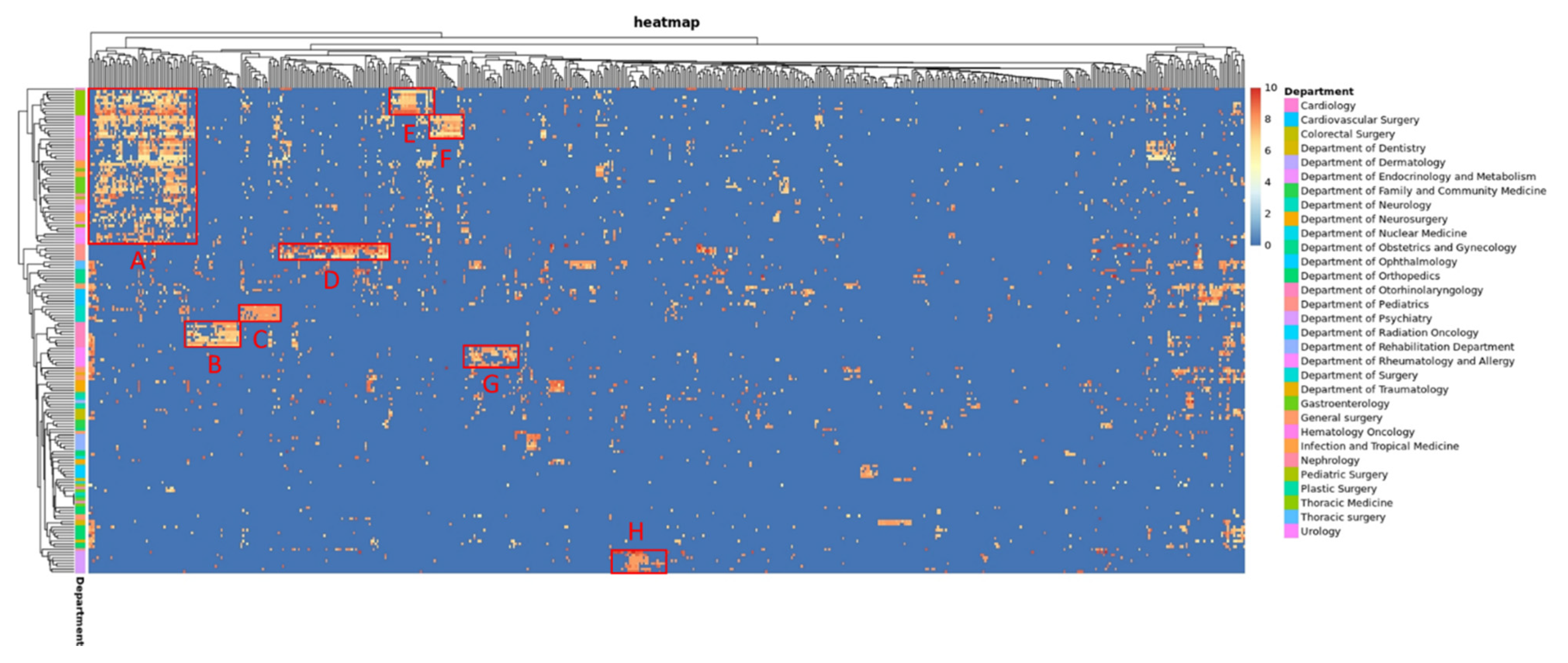
| Block | Experts’ Score (a) | BERT Score (b) | LSTM Score (c) | p-Value | LMM-Modified BERT Score (d) | LMM-Modified LSTM Score (e) | p-Value | |a-b| # | |a-d| # | p-Value | |a-c| # | |a-e| # | p-Value |
|---|---|---|---|---|---|---|---|---|---|---|---|---|---|
| A | 7.44 ± 0.66 | 7.35 ± 0.17 | 6.99 ± 0.17 | <0.001 * | 7.08 ± 0.56 | 7.02 ± 0.66 | 0.626 | 0.83 ± 0.27 | 0.66 ± 0.38 | 0.008 * | 0.97 ± 0.33 | 0.63 ± 0.43 | <0.001 * |
| B | 7.35 ± 0.51 | 7.43 ± 0.06 | 7.32 ± 0.17 | 0.087 | 7.32 ± 0.47 | 7.38 ± 0.54 | 0.824 | 0.7 ± 0.13 | 0.51 ± 0.17 | 0.013 * | 0.76 ± 0.16 | 0.45 ± 0.2 | 0.002 * |
| C | 7.88 ± 0.14 | 7.56 ± 0.09 | 7.4 ± 0.1 | 0.016 * | 7.59 ± 0.18 | 7.63 ± 0.24 | 0.740 | 0.69 ± 0.03 | 0.54 ± 0.1 | 0.005 * | 0.77 ± 0.08 | 0.41 ± 0.14 | <0.001 * |
| D | 7.94 ± 1 | 7.43 ± 0.19 | 7.13 ± 0.08 | 0.005 * | 7.57 ± 0.6 | 7.61 ± 0.84 | 0.932 | 1.29 ± 0.29 | 0.88 ± 0.31 | 0.042 * | 1.44 ± 0.3 | 0.74 ± 0.35 | 0.004 * |
| E | 7.74 ± 0.91 | 7.51 ± 0.08 | 6.98 ± 0.18 | <0.001 * | 7.19 ± 0.45 | 7.12 ± 0.56 | 0.772 | 1.05 ± 0.33 | 0.85 ± 0.4 | 0.227 | 1.25 ± 0.41 | 0.8 ± 0.35 | 0.016 * |
| F | 7.3 ± 0.63 | 6.97 ± 0.24 | 6.61 ± 0.17 | 0.004 * | 6.75 ± 0.54 | 6.69 ± 0.74 | 0.874 | 0.88 ± 0.22 | 0.73 ± 0.28 | 0.258 | 1 ± 0.27 | 0.78 ± 0.3 | 0.154 |
| G | 7.76 ± 0.15 | 7.46 ± 0.08 | 7.08 ± 0.11 | <0.001 * | 7.52 ± 0.25 | 7.46 ± 0.37 | 0.707 | 0.69 ± 0.08 | 0.63 ± 0.12 | 0.238 | 0.93 ± 0.12 | 0.6 ± 0.2 | 0.003 * |
| H | 8.41 ± 0.47 | 8.1 ± 0.06 | 8.05 ± 0.18 | 0.436 | 7.93 ± 0.59 | 7.95 ± 0.67 | 0.962 | 0.71 ± 0.23 | 0.58 ± 0.48 | 0.489 | 1 ± 0.3 | 0.51 ± 0.55 | 0.045 * |
Publisher’s Note: MDPI stays neutral with regard to jurisdictional claims in published maps and institutional affiliations. |
© 2021 by the authors. Licensee MDPI, Basel, Switzerland. This article is an open access article distributed under the terms and conditions of the Creative Commons Attribution (CC BY) license (https://creativecommons.org/licenses/by/4.0/).
Share and Cite
Lin, C.; Lee, Y.-T.; Wu, F.-J.; Lin, S.-A.; Hsu, C.-J.; Lee, C.-C.; Tsai, D.-J.; Fang, W.-H. The Application of Projection Word Embeddings on Medical Records Scoring System. Healthcare 2021, 9, 1298. https://doi.org/10.3390/healthcare9101298
Lin C, Lee Y-T, Wu F-J, Lin S-A, Hsu C-J, Lee C-C, Tsai D-J, Fang W-H. The Application of Projection Word Embeddings on Medical Records Scoring System. Healthcare. 2021; 9(10):1298. https://doi.org/10.3390/healthcare9101298
Chicago/Turabian StyleLin, Chin, Yung-Tsai Lee, Feng-Jen Wu, Shing-An Lin, Chia-Jung Hsu, Chia-Cheng Lee, Dung-Jang Tsai, and Wen-Hui Fang. 2021. "The Application of Projection Word Embeddings on Medical Records Scoring System" Healthcare 9, no. 10: 1298. https://doi.org/10.3390/healthcare9101298