
Unboxing Industry-Standard AI Models for Male Fertility Prediction with SHAP


Abstract
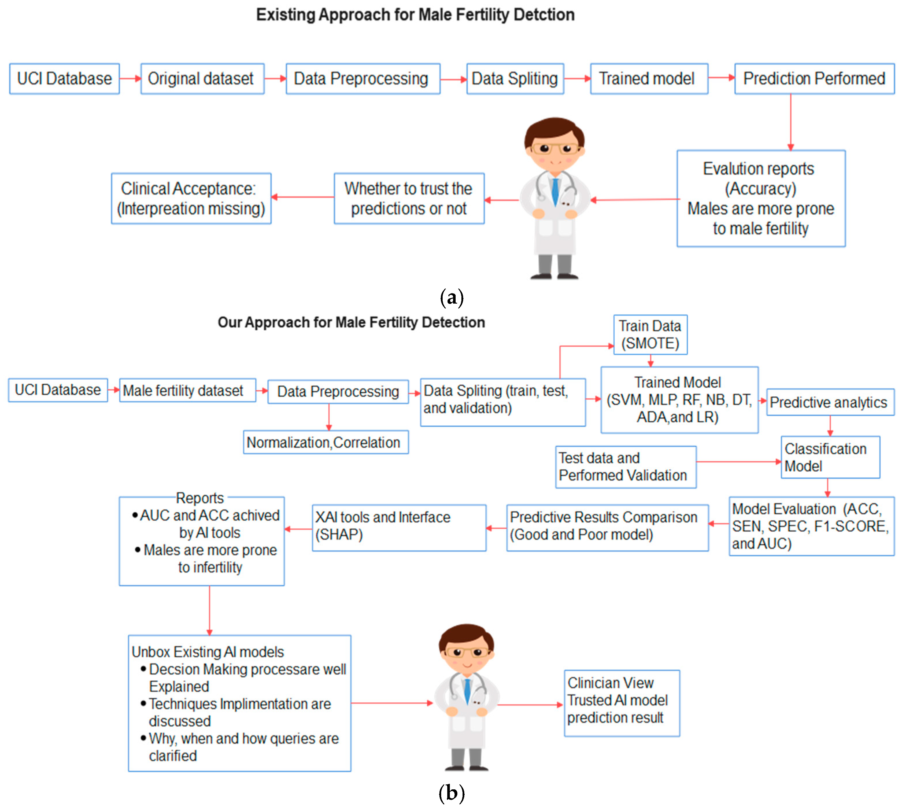
:1. Introduction
- Seven industry-standard ML models are analyzed for male fertility detection.
- To assess the robustness and stability of each model, we employ sampling and two different CV techniques on each AI model.
- XAI is used to explain the performance of each good and poor model and uncover the black box.
2. Problem Background
2.1. Class Imbalance Learning
2.1.1. Small Sample Size
2.1.2. Class Overlapping
2.1.3. Small Disjuncts
2.2. Sampling Approaches
2.3. Classifier Selection
2.4. Validation Schemes
2.5. XAI Tools
3. Material and Methods
3.1. Data Source and Information
3.2. Analysis of Dataset
3.2.1. Statistical Overview
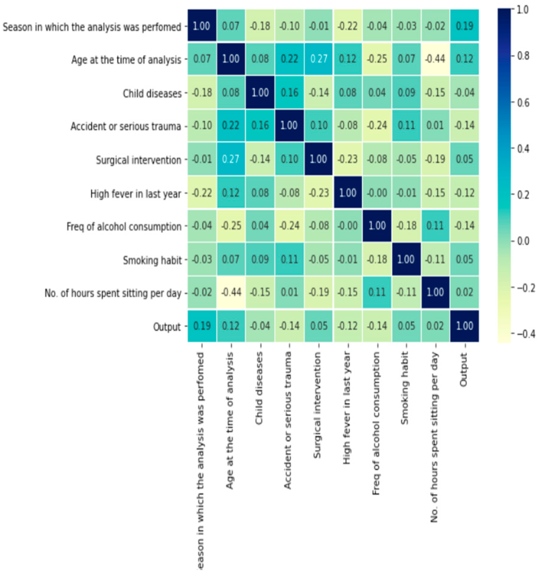
3.2.2. Measure of Relationship
3.3. Sampling Technique
3.4. Overview of Classification Models
3.4.1. SVM
3.4.2. RF
3.4.3. DT
3.4.4. LR
3.4.5. NB
3.4.6. ADA
3.4.7. MLP
3.5. Validation Schemes and Performance Metrics
3.5.1. Validation Schemes
3.5.2. Performance Metrics
3.6. SHAP
4. Results and Analysis
4.1. Performance of the Models with the Imbalanced Dataset
4.2. Performance of the Models with a Balanced Dataset
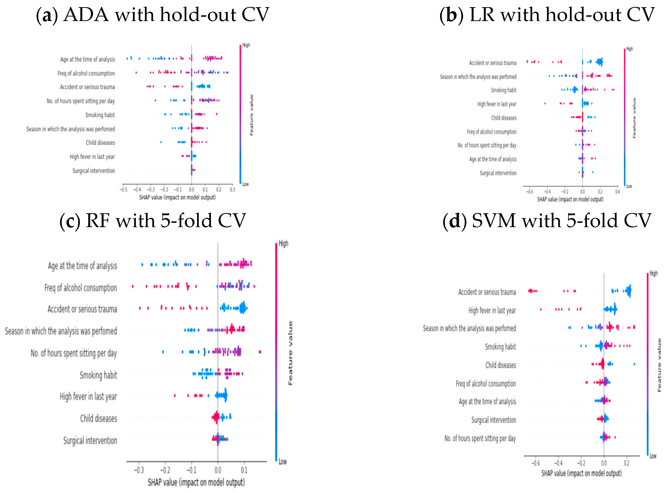
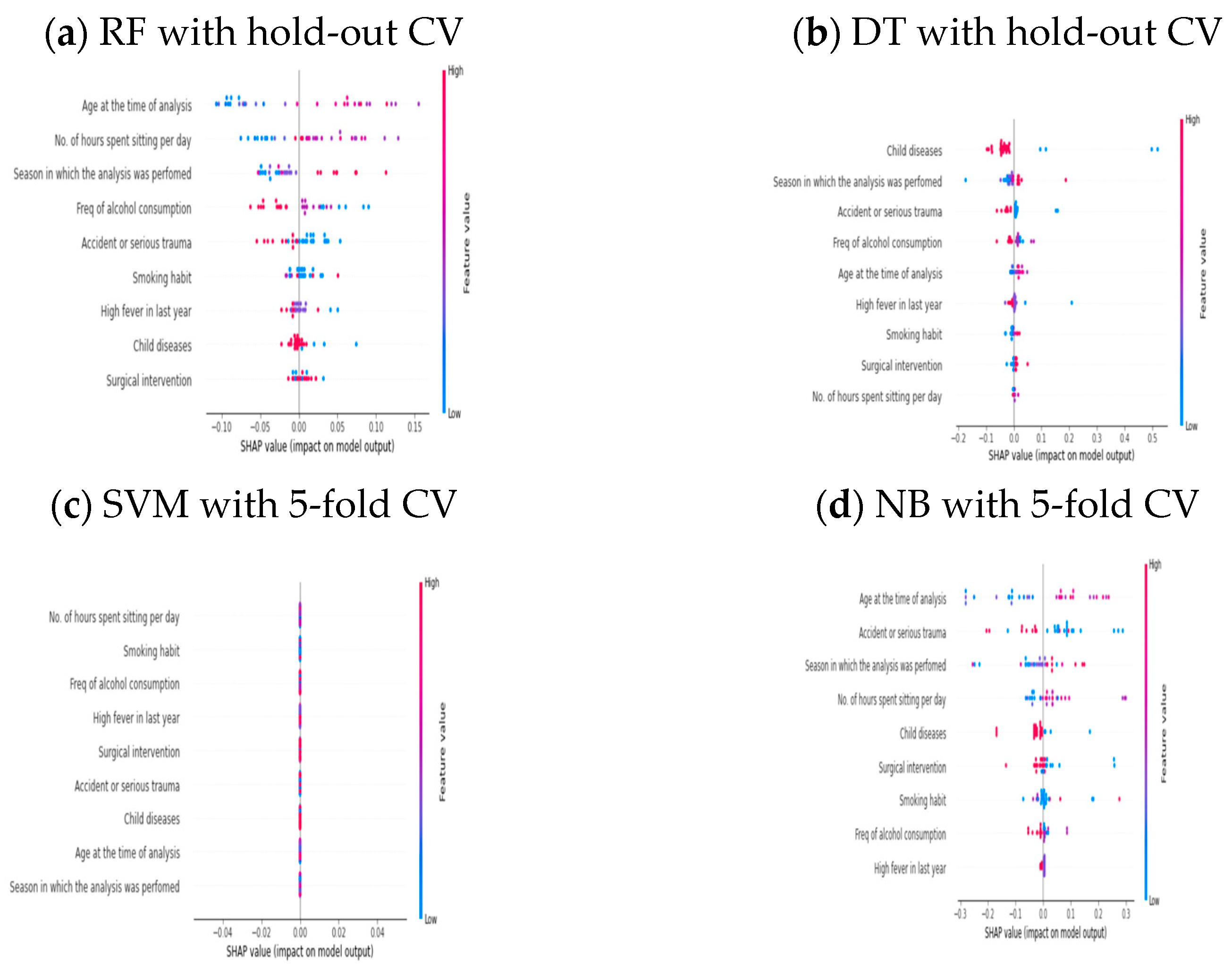
4.3. Unboxing the Good and Poorly Performed AI Models via SHAP on a Balanced Dataset
4.4. Unboxing the Good and Poorly Performed AI Models via SHAP on an Imbalanced Dataset
5. Discussion
6. Conclusions
Author Contributions
Funding
Institutional Review Board Statement
Informed Consent Statement
Data Availability Statement
Conflicts of Interest
Correction Statement
Abbreviations
| True Positive | |
| True Negative | |
| False Positive | |
| False Negative | |
| True Positive Rate | |
| False Positive Rate |
Appendix A

| Dataset | Methods | AUCs | |
|---|---|---|---|
| Training | Validation | ||
| Balanced | 5-fold CV | 1.0 | 0.97 |
References
- Chen, T.; Belladelli, F.; Del Giudice, F.; Eisenberg, M.L. Male fertility as a marker for health. Reprod. BioMed. Online 2022, 44, 131–144. [Google Scholar] [CrossRef] [PubMed]
- Durairajanayagam, D. Lifestyle causes of male infertility. Arab J. Urol. 2018, 16, 10–20. [Google Scholar] [CrossRef]
- Mendiola, J.; Torres-Cantero, A.M.; Agarwal, A. Lifestyle factors and male infertility: An evidence-based review. Arch. Med. Sci. Spec. Issues 2009, 2009, 12. [Google Scholar]
- Kumar, N.; Singh, A.K. Impact of environmental factors on human semen quality and male fertility: A narrative review. Environ. Sci. Eur. 2022, 34, 6. [Google Scholar] [CrossRef]
- Dimitriadis, I.; Zaninovic, N.; Badiola, A.C.; Bormann, C.L. Artificial intelligence in the embryology laboratory: A review. Reprod. BioMed Online 2022, 44, 435–448. [Google Scholar] [CrossRef]
- Medenica, S.; Zivanovic, D.; Batkoska, L.; Marinelli, S.; Basile, G.; Perino, A.; Zaami, S. The Future Is Coming: Artificial Intelligence in the Treatment of Infertility Could Improve Assisted Reproduction Outcomes—The Value of Regulatory Frameworks. Diagnostics 2022, 12, 2979. [Google Scholar] [CrossRef] [PubMed]
- Gil, D.; Girela, J.L.; De Juan, J.; Gomez-Torres, M.J.; Johnsson, M. Predicting seminal quality with artificial intelligence methods. Expert Syst. Appl. 2012, 39, 12564–12573. [Google Scholar] [CrossRef]
- Sahoo, A.J.; Kumar, Y. Seminal quality prediction using data mining methods. Technol. Health Care 2014, 22, 531–545. [Google Scholar] [CrossRef] [PubMed]
- Bidgoli, A.A.; Komleh, H.E.; Mousavirad, S.J. Seminal quality prediction using optimized artificial neural network with genetic algorithm. In Proceedings of the 9th International Conference on Electrical and Electronics Engineering (ELECO), Bursa, Turkey, 26–28 November 2015; IEEE: New York, NY, USA, 2015; pp. 695–699. [Google Scholar]
- Girela, J.L.; Gil, D.; Johnsson, M.; Gomez-Torres, M.J.; De Juan, J. Semen parameters can be predicted from environmental factors and lifestyle using artificial intelligence methods. Biol. Reprod. 2013, 88, 1–8. [Google Scholar] [CrossRef] [PubMed]
- Soltanzadeh, S.; Zarandi, M.H.F.; Astanjin, M.B. A hybrid fuzzy clustering approach for fertile and unfertile analysis. In Proceedings of the Annual Conference of the North American Fuzzy Information Processing Society (NAFIPS), El Paso, TX, USA, 31 October–4 November 2016; IEEE: New York, NY, USA, 2016; pp. 1–6. [Google Scholar]
- Rhemimet, A.; Raghay, S.; Bencharef, O. Comparative Analysis of Classification, Clustering and Regression Techniques to Explore Men’s Fertility. In Proceedings of the Mediterranean Conference on Information & Communication Technologies, Saidia, Morocco, 7–9 May 2015; Springer: Cham, Switzerland, 2016; pp. 455–462. [Google Scholar]
- Candemir, C. Estimating the semen quality from life style using fuzzy radial basis functions. Int. J. Mach. Learn. Comput. 2018, 8, 44–48. [Google Scholar] [CrossRef]
- Simfukwe, M.; Kunda, D.; Chembe, C. Comparing naive bayes method and artificial neural network for semen quality categorization. Int. J. Innov. Sci. Eng. Technol. 2015, 2, 689–694. [Google Scholar]
- Prediction of Seminal Quality Based on Naïve Bayes Approach. Available online: https://www.academia.edu/43543009/Prediction_of_Seminal_Quality_Based_on_Na%C3%AFve_Bayes_Approach (accessed on 10 September 2022).
- Engy, E.L.; Ali, E.L.; Sally, E.G. An optimized artificial neural network approach based on sperm whale optimization algorithm for predicting fertility quality. Stud. Inform. Control 2018, 27, 349–358. [Google Scholar]
- Mendoza-Palechor, F.E.; Ariza-Colpas, P.P.; Sepulveda-Ojeda, J.A.; De-la-Hoz-Manotas, A.; Piñeres Melo, M. Fertility analysis method based on supervised and unsupervised data mining techniques. Int. J. Appl. Eng. Res. 2016, 11, 10374–10379. [Google Scholar]
- Ma, J.; Afolabi, D.O.; Ren, J.; Zhen, A. Predicting seminal quality via imbalanced learning with evolutionary safe-level synthetic minority over-sampling technique. Cogn. Comput. 2019, 13, 833–844. [Google Scholar] [CrossRef]
- Dash, S.R.; Ray, R. Predicting seminal quality and its dependence on life style factors through ensemble learning. Int. J. E-Health Med. Commun. IJEHMC 2020, 11, 78–95. [Google Scholar] [CrossRef]
- Roy, D.G.; Alvi, P.A. Detection of Male Fertility Using AI-Driven Tools. In International Conference on Recent Trends in Image Processing and Pattern Recognition; Springer: Cham, Switzerland, 2022; pp. 14–25. [Google Scholar]
- Yibre, A.M.; Koçer, B. Semen quality predictive model using Feed Forwarded Neural Network trained by Learning-Based Artificial Algae Algorithm. Eng. Sci. Technol. Int. J. 2021, 24, 310–318. [Google Scholar] [CrossRef]
- GhoshRoy, D.; Alvi, P.A.; Santosh, K.C. Explainable AI to Predict Male Fertility Using Extreme Gradient Boosting Algorithm with SMOTE. Electronics 2022, 12, 15. [Google Scholar] [CrossRef]
- Santos, M.S.; Abreu, P.H.; Japkowicz, N.; Fernández, A.; Soares, C.; Wilk, S.; Santos, J. On the joint-effect of class imbalance and overlap: A critical review. Artif. Intell. Rev. 2022, 1–69. [Google Scholar]
- Susan, S.; Kumar, A. The balancing trick: Optimized sampling of imbalanced datasets—A brief survey of the recent State of the Art. Eng. Rep. 2021, 3, e12298. [Google Scholar] [CrossRef]
- Li, J.; Zhu, Q.; Wu, Q.; Fan, Z. A novel oversampling technique for class-imbalanced learning based on SMOTE and natural neighbors. Inf. Sci. 2021, 565, 438–455. [Google Scholar] [CrossRef]
- Bunkhumpornpat, C.; Sinapiromsaran, K.; Lursinsap, C. Safe-level-smote: Safe-level-synthetic minority over-sampling technique for handling the class imbalanced problem. In Advances in Knowledge Discovery and Data Mining, Proceedings of the 13th Pacific-Asia Conference, PAKDD 2009, Bangkok, Thailand, 27–30 April 2009; Springer: Berlin/Heidelberg, Germany, 2009; pp. 475–482. [Google Scholar]
- Lenselink, C.; Ties, D.; Pleijhuis, R.; van der Harst, P. Validation and comparison of 28 risk prediction models for coronary artery disease. Eur. J. Prev. Cardiol. 2022, 29, 666–674. [Google Scholar] [CrossRef]
- Loh, H.W.; Ooi, C.P.; Seoni, S.; Barua, P.D.; Molinari, F.; Acharya, U.R. Application of explainable artificial intelligence for healthcare: A systematic review of the last decade (2011–2022). Comput. Methods Programs Biomed. 2022, 226, 107161. [Google Scholar] [CrossRef]
- Chawla, N.V.; Bowyer, K.W.; Hall, L.O.; Kegelmeyer, W.P. SMOTE: Synthetic Minority Over-sampling Technique. J. Artif. Intell. Res. 2002, 16, 321–357. [Google Scholar] [CrossRef]
- Cortes, C.; Vapnik, V. Support-vector networks. Mach. Learn. 1995, 20, 273–297. [Google Scholar] [CrossRef]
- Ho, T.K. Random Decision Forest. In Proceedings of the 3rd International Conference on Document Analysis and Recognition, Montreal, QC, Canada, 14–16 August 1995; pp. 278–282. [Google Scholar]
- Amit, Y.; Geman, D. Shape Quantization and Recognition with Randomized Trees. Neural Comput. 1997, 9, 1545–1588. [Google Scholar] [CrossRef]
- Breiman, L. Random forests. Mach. Learn. 2001, 45, 5–32. [Google Scholar] [CrossRef]
- Quinlan, J.R. Induction of decision trees. Mach. Learn. 1986, 1, 81–106. [Google Scholar] [CrossRef]
- Msaouel, P.; Jimenez-Fonseca, P.; Lim, B.; Carmona-Bayonas, A.; Agnelli, G. Medicine before and after David Cox. Eur. J. Intern. Med. 2022, 98, 1–3. [Google Scholar] [CrossRef]
- Jiang, L.; Zhang, H.; Cai, Z. A novel Bayes model: Hidden naive Bayes. IEEE Trans. Knowl. Data Eng. 2008, 21, 1361–1371. [Google Scholar] [CrossRef]
- Freund, Y.; Schapire, R.; Abe, N. A short introduction to boosting. J.-Jpn. Soc. Artif. Intell. 1999, 14, 1612. [Google Scholar]
- Ying, C.; Qi-Guang, M.; Jia-Chen, L.; Lin, G. Advance and prospects of AdaBoost algorithm. Acta Autom. Sin. 2013, 39, 745–758. [Google Scholar]
- Rosenblatt, F. Principles of Neurodynamics. Perceptrons and the Theory of Brain Mechanisms; Cornell Aeronautical Lab. Inc.: Buffalo, NY, USA, 1961. [Google Scholar]
- Refaeilzadeh, P.; Tang, L.; Liu, H. Cross-validation. Encycl. Database Syst. 2009, 5, 532–538. [Google Scholar]
- Wong, T.T.; Yeh, P.Y. Reliable accuracy estimates from k-fold cross validation. IEEE Trans. Knowl. Data Eng. 2019, 32, 1586–1594. [Google Scholar] [CrossRef]
- Costello, M.F.; Sjoblom, P.; Haddad, Y.; Steigrad, S.J.; Bosch, E.G. No decline in semen quality among potential sperm donors in Sydney, Australia, between 1983 and 2001. J. Assist. Reprod. Genet. 2002, 19, 284–290. [Google Scholar] [CrossRef]
- Ekanayake, I.U.; Meddage DP, P.; Rathnayake, U. A novel approach to explain the black-box nature of machine learning in compressive strength predictions of concrete using Shapley additive explanations (SHAP). Case Stud. Constr. Mater. 2022, 16, e01059. [Google Scholar] [CrossRef]
- Van den Broeck, G.; Lykov, A.; Schleich, M.; Suciu, D. On the tractability of SHAP explanations. J. Artif. Intell. Res. 2022, 74, 851–886. [Google Scholar] [CrossRef]
- Eisenberg, M.L.; Murthy, L.; Hwang, K.; Lamb, D.J.; Lipshultz, L.I. Sperm counts and sperm sex ratio in male infertility patients. Asian J. Androl. 2012, 14, 683. [Google Scholar] [CrossRef]
- Li, W.N.; Jia, M.M.; Peng, Y.Q.; Ding, R.; Fan, L.Q.; Liu, G. Semen quality pattern and age threshold: A retrospective cross-sectional study of 71,623 infertile men in China, between 2011 and 2017. Reprod. Biol. Endocrinol. 2019, 17, 107. [Google Scholar] [CrossRef]
- Liao, W.B.; Zhong, M.J.; Lüpold, S. Sperm quality and quantity evolve through different selective processes in the Phasianidae. Sci. Rep. 2019, 9, 19278. [Google Scholar] [CrossRef]


| Features. No | Feature’s Name | Values Range (Max–Min) | Normalized |
|---|---|---|---|
| Season | winter, spring, summer, and fall | (−1, −0.33, 0.33, 1) | |
| Age | 18–36 | (0, 1) | |
| Childhood Disease | yes or no | (0, 1) | |
| Accident/Trauma | yes or no | (0, 1) | |
| Surgical Interventional | yes or no | (0, 1) | |
| High Fever | less than 3 months ago, more than 3 months ago, no | (−1, 0, 1) | |
| Alcohol Intake | several times a day, every day, several times in a week, and hardly ever or never | (0, 1) | |
| Smoking Habit | never, occasional, and daily | (−1, 0, 1) | |
| Sitting Hours/day | 1–16 | (0, 1) | |
| Target Class | normal or altered | (1, 0) |
| Count | 100.000000 | 100.000000 | 100.000000 | 100.000000 | 100.000000 | 100.000000 | 100.000000 | 100.000000 | 100.000000 | 100.000000 |
| Mean | −0.078900 | 0.669000 | 0.870000 | 0.440000 | 0.510000 | 0.190000 | 0.832000 | −0.350000 | 0.406800 | 1.120000 |
| Std | 0.796725 | 0.121319 | 0.337998 | 0.498888 | 0.502418 | 0.580752 | 0.167501 | 0.808728 | 0.186395 | 0.326599 |
| Min | −1.000000 | 0.500000 | 0.000000 | 0.000000 | 0.000000 | −1.000000 | −0.200000 | −1.000000 | 0.060000 | 1.000000 |
| 25% | −1.000000 | 0.560000 | 1.000000 | 0.000000 | 0.000000 | 0.000000 | 0.800000 | −1.000000 | 0.250000 | 1.000000 |
| 50% | −0.330000 | 0.670000 | 1.000000 | 0.000000 | 1.000000 | 0.000000 | 0.800000 | −1.000000 | 0.380000 | 1.000000 |
| 75% | 1.000000 | 0.750000 | 1.000000 | 1.000000 | 1.000000 | 1.000000 | 1.000000 | 0.000000 | 0.500000 | 1.000000 |
| Max | 1.000000 | 1.000000 | 1.000000 | 1.000000 | 1.000000 | 1.000000 | 1.000000 | 1.000000 | 1.000000 | 2.000000 |
| 1.000000 | 0.065410 | −0.176509 | −0.096274 | −0.006210 | −0.221818 | −0.041290 | −0.028085 | −0.019021 | 0.192417 | |
| 0.065410 | 1.000000 | 0.080551 | 0.215958 | 0.271945 | 0.120284 | −0.247940 | 0.072581 | −0.442452 | 0.115229 | |
| −0.176509 | 0.080551 | 1.000000 | 0.162936 | −0.140972 | 0.075645 | 0.038538 | 0.090535 | −0.147761 | −0.040261 | |
| −0.096274 | 0.215958 | 0.162936 | 1.000000 | 0.103166 | −0.082278 | −0.242722 | 0.110157 | 0.013122 | −0.141346 | |
| −0.006210 | 0.271945 | −0.140972 | 0.103166 | 1.000000 | −0.231598 | −0.075858 | −0.053448 | −0.192726 | 0.054171 | |
| −0.221818 | 0.120284 | 0.075645 | −0.082278 | −0.231598 | 1.000000 | −0.000831 | −0.007527 | −0.151091 | −0.121421 | |
| −0.041290 | −0.247940 | 0.038538 | −0.242722 | −0.075858 | −0.000831 | 1.000000 | −0.184926 | 0.111371 | −0.144760 | |
| −0.028085 | 0.072581 | 0.090535 | 0.110157 | −0.053448 | −0.007527 | −0.184926 | 1.000000 | −0.106007 | 0.045891 | |
| −0.019021 | −0.442452 | −0.147761 | 0.013122 | −0.192726 | −0.151091 | 0.111371 | −0.106007 | 1.000000 | 0.022964 | |
| 0.192417 | 0.115229 | −0.040261 | −0.141346 | 0.054171 | −0.121421 | −0.144760 | 0.045891 | 0.022964 | 1.000000 |
| Target Class | Before SMOTE | Total Data Size | After SMOTE | Training Data Size |
|---|---|---|---|---|
| Normal sperm quality | 88 | 100 | 88 | 172 |
| Altered sperm quality | 12 | 84 |
| Models | Test Set Performances | ||||
|---|---|---|---|---|---|
| ACC (in%) | SEN | SPEC | F1-Score | AUC | |
| SVM | 93.33 | 0.933 | 0.091 | 0.965 | 0.887 |
| RF | 96.67 | 0.965 | 0.965 | 0.982 | 0.932 |
| DT | 80.00 | 0.956 | 0.142 | 0.863 | 0.648 |
| LR | 93.33 | 0.931 | 0.098 | 0.965 | 0.862 |
| NB | 86.66 | 0.928 | 0.079 | 0.928 | 0.664 |
| ADA | 93.33 | 0.964 | 0.599 | 0.964 | 0.908 |
| MLP | 93.30 | 0.965 | 0.548 | 0.964 | 0.746 |
| Models | Test Set Performances | |||||
|---|---|---|---|---|---|---|
| ACC (in%) | SEN | SPEC | F1-Score | STD | AUC | |
| SVM | 88.00 | 1.000 | 0.997 | 0.965 | 0.024 | 0.959 |
| RF | 87.99 | 0.943 | 0.711 | 0.982 | 0.070 | 0.720 |
| DT | 74.99 | 0.817 | 0.670 | 0.884 | 0.141 | 0.625 |
| LR | 88.00 | 1.000 | 0.817 | 0.965 | 0.024 | 0.910 |
| NB | 67.00 | 0.734 | 0.570 | 0.928 | 0.299 | 0.500 |
| MLP | 80.99 | 0.809 | 0.742 | 0.964 | 0.050 | 0.694 |
| ADA | 80.00 | 0.884 | 0.933 | 0.964 | 0.141 | 0.839 |
| Methods | Test Set Performances | ||||
|---|---|---|---|---|---|
| ACC (in%) | SEN | SPEC | F1-Score | AUC | |
| SVM | 84.90 | 0.951 | 0.789 | 0.826 | 0.807 |
| RF | 92.45 | 0.958 | 0.838 | 0.919 | 0.940 |
| DT | 84.09 | 0.909 | 0.806 | 0.833 | 0.798 |
| LR | 83.01 | 0.905 | 0.781 | 0.808 | 0.704 |
| NB | 88.67 | 0.954 | 0.839 | 0.875 | 0.749 |
| MLP | 83.01 | 0.904 | 0.781 | 0.808 | 0.801 |
| ADA | 96.15 | 0.9615 | 0.962 | 0.961 | 0.966 |
| Models | Test Set Performances | |||||
|---|---|---|---|---|---|---|
| ACC (in%) | SEN | SPEC | F1-Score | STD | AUC | |
| SVM | 81.92 | 0.706 | 0.808 | 0.826 | 0.097 | 0.737 |
| RF | 90.47 | 0.909 | 0.999 | 0.919 | 0.133 | 0.998 |
| DT | 85.87 | 0.830 | 0.897 | 0.833 | 0.070 | 0.741 |
| LR | 82.47 | 0.752 | 0.879 | 0.809 | 0.088 | 0.763 |
| NB | 85.87 | 0.797 | 0.863 | 0.876 | 0.108 | 0.750 |
| MLP | 85.90 | 0.762 | 0.848 | 0.809 | 0.113 | 0.796 |
| ADA | 87.01 | 0.826 | 0.817 | 0.962 | 0.096 | 0.893 |
| Dataset | Models | CV Schemes | Test ACC (in %) | Test AUC |
|---|---|---|---|---|
| Balanced | ADA | Hold-out | 96.15 | 0.966 |
| RF | 5-fold | 90.47 | 0.998 | |
| Imbalanced | RF | Hold-out | 96.67 | 0.932 |
| SVM | 5-fold | 88.00 | 0.959 |
| Dataset | Methods | CV Schemes | Test ACC (in %) | Test AUC |
|---|---|---|---|---|
| Balanced | LR | Hold-out | 83.01 | 0.774 |
| SVM | 5-fold | 81.92 | 0.737 | |
| Imbalanced | DT | Hold-out | 80.00 | 0.648 |
| NB | 5-fold | 67.00 | 0.500 |
| Models | ACC (in %) | SEN | SPEC | F1-Score | AUC | Remarks |
|---|---|---|---|---|---|---|
| SVM, MLP, and DT [7] | 86, 86 and 84 (SC), 69, 69, 67 (SM) | 94.0, 97.0, 96.0 (SC) 72.0, 73.0, 71.0 (SM) | 40.0, 20.0, 13.0 (SC) 25.0, 12.0, 12.0 (SM) | - | - | SC = Sperm morphology. SM = Sperm concentration individually measured |
| DT, MLP, SVM, SVM-PSO, and NB [8] | 89, 92, 91, 94, and 89 | - | - | - | 73.5, 72.8, 75.8, 93.2, and 85.0 | Feature selection applied |
| MLP, NB, DT, and SVM [9] | 93.3, 73.10, 83.82, and 80.88 | - | - | - | 93.3, 81.0, 85.8, 88.2 | Optimize MLP |
| MLP [10] | 90, and 82 | 95.4 and 89.2 | 50 and 43.7 | - | - | - |
| NB, NN, LR, and Fuzzy C-means [11] | - | - | - | - | 75.1, 78.2, 46.6, 69.0 | Filtering applied |
| DT and NB [12] | 61.36 and 88.63 | - | - | - | - | |
| MLP, SVM, DT, and FRBF [13] | 69.0, 69.0, 67, and 90 | 72.0, 73.0, 71.0, and 92.0 | 25.0, 12.0, 12.0, and 50.0 | - | - | |
| ANN and NB [14] | 97 | - | - | - | - | Testing accuracy not reported |
| NB [15] | 87.75 | - | - | - | - | - |
| ANN, ANN-GA, DT, SVM, and ANN-SWA [16] | 90, 95, 88, 95, and 99.96 | 92.0, 97.0, 83.0, 97.0, and 99.0 | 71.0, 70.0, 82.0, 72.0, and 99.0 | - | - | |
| J48, SMO, NB, and lazy IBK [17] | - | - | - | - | - | Classification and clustering performed |
| SVM, AdaBoost, and BPNN [18] | 81.6, 95.1, and 91.6 | - | - | 91.3, 97.2, and 91.6 | - | ELSMOTE is used |
| DT, Bagged DT, RF, and ET [19] | 78.80, 88.12, 89.07, and 90.02 | - | - | 66 (ET) | - | Not reported all models of AUC |
| KNN [20] | 90.00 | - | - | - | 85.7 | - |
| MLP, SVM, NB, RF, KNN, and FFNN-LBAAA [21] | 81, 72, 87.2, 91.3, 84.9, and 97.5 | 75.0, 69.0, 90.0, 92.0, 81.0, and 93.0 | 87.0, 74.0, 85.0, 90.0, 89.0, and 100 | 80.0, 71.3,87.8,91.5,84.5, and 96.6 | 81.0, 72.0, 87.0, 91.0, 85.0, and 97.0 | SMOTE is used |
| XGB [22] | 93.22 | 95.0 | 95.0 | - | 98.0 | SMOTE and XAI tools are used |
| RF _XAI * | 90.47 | 90.98 | 99.99 | 91.99 | 99.98 | 5-fold CV, SMOTE, and SHAP used |
| Performance | Methods | CV Schemes | Feature’s Role |
|---|---|---|---|
| Good | ADA-SMOTE | Hold-out | , , |
| RF-SMOTE | Five-fold | , , | |
| RF | Hold-out | , , | |
| SVM | Five-fold | , , | |
| Poor | LR-SMOTE | Hold-out | , , |
| SVM-SMOTE | Five-fold | , , | |
| DT | Hold-out | , , | |
| NB | Five-fold | , , |
Disclaimer/Publisher’s Note: The statements, opinions and data contained in all publications are solely those of the individual author(s) and contributor(s) and not of MDPI and/or the editor(s). MDPI and/or the editor(s) disclaim responsibility for any injury to people or property resulting from any ideas, methods, instructions or products referred to in the content. |
© 2023 by the authors. Licensee MDPI, Basel, Switzerland. This article is an open access article distributed under the terms and conditions of the Creative Commons Attribution (CC BY) license (https://creativecommons.org/licenses/by/4.0/).
Share and Cite
GhoshRoy, D.; Alvi, P.A.; Santosh, K. Unboxing Industry-Standard AI Models for Male Fertility Prediction with SHAP. Healthcare 2023, 11, 929. https://doi.org/10.3390/healthcare11070929
GhoshRoy D, Alvi PA, Santosh K. Unboxing Industry-Standard AI Models for Male Fertility Prediction with SHAP. Healthcare. 2023; 11(7):929. https://doi.org/10.3390/healthcare11070929
Chicago/Turabian StyleGhoshRoy, Debasmita, Parvez Ahmad Alvi, and KC Santosh. 2023. "Unboxing Industry-Standard AI Models for Male Fertility Prediction with SHAP" Healthcare 11, no. 7: 929. https://doi.org/10.3390/healthcare11070929