
Intelligent Deep-Learning-Enabled Decision-Making Medical System for Pancreatic Tumor Classification on CT Images

 , , ,
, , ,
Abstract
:1. Introduction
2. Literature Review
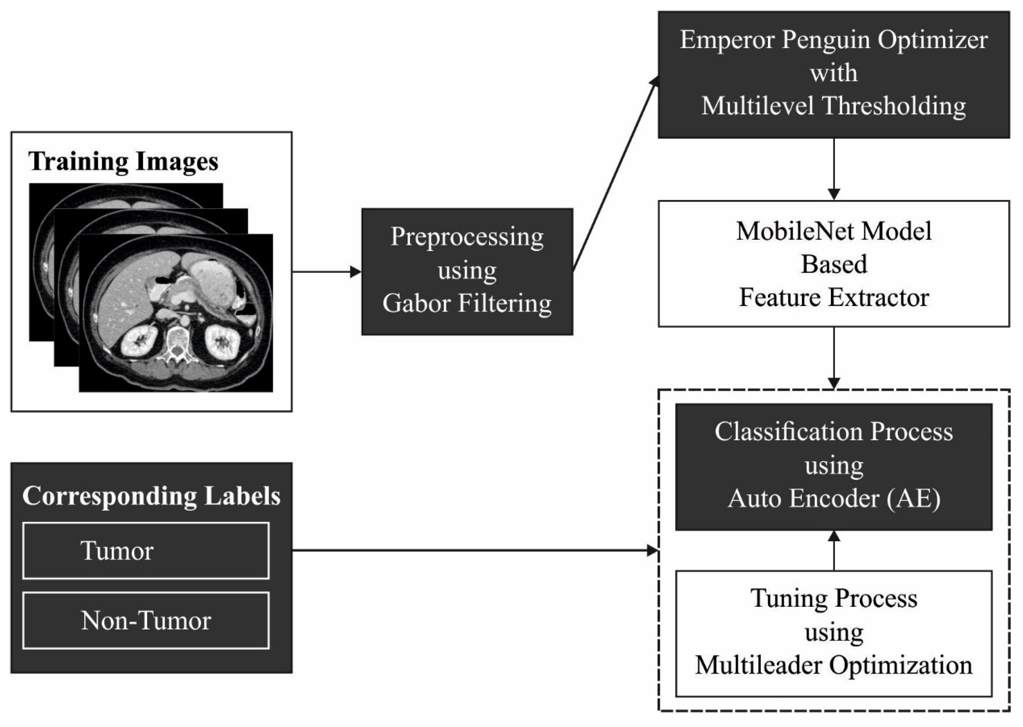
3. The Proposed Model
3.1. Gabor Filtering Based Pre-Processing
3.2. EPO-MLT-Based Segmentation
3.3. MobileNet-Based Feature Extraction
3.4. Optimal AE-Based Classification
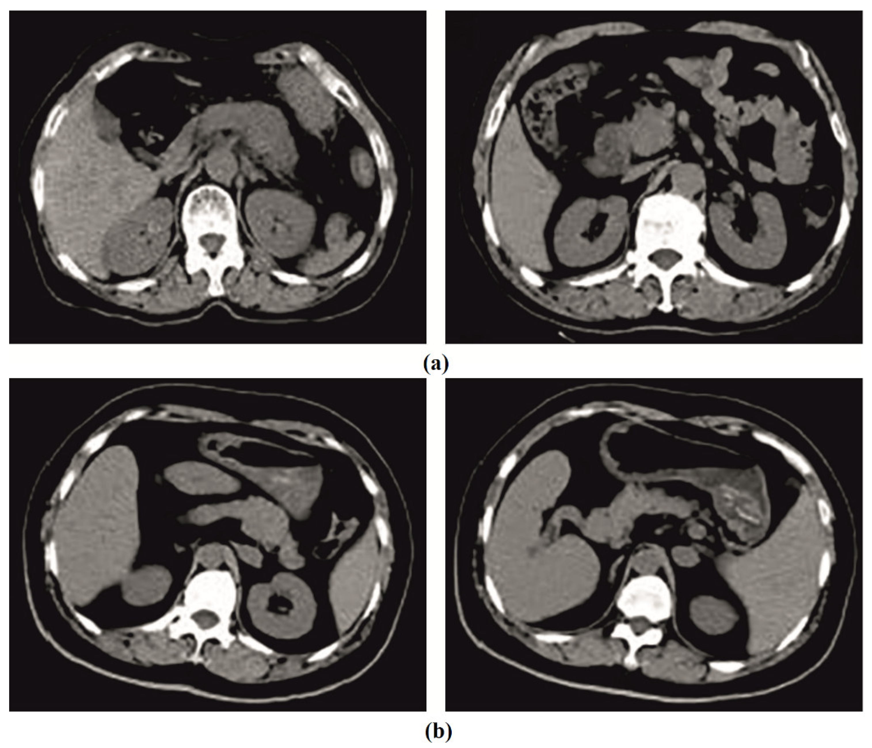
4. Experimental Validation
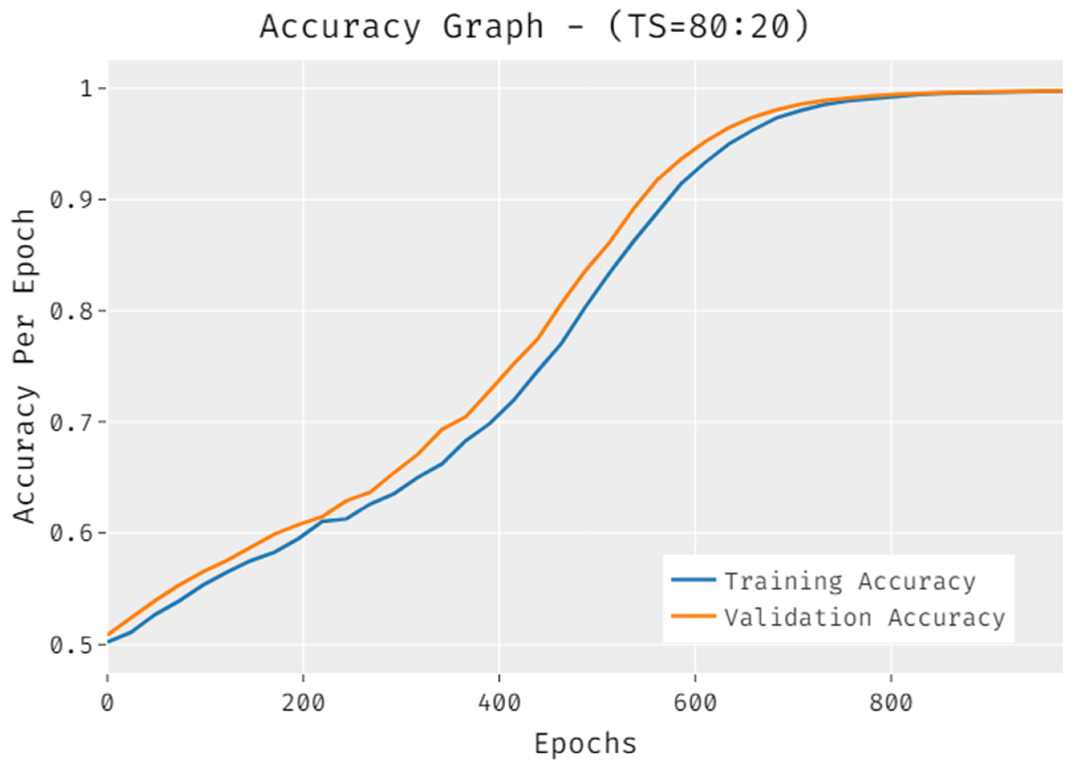
4.1. Results Analysis
4.2. Discussion
5. Conclusions
Author Contributions
Funding
Institutional Review Board Statement
Informed Consent Statement
Data Availability Statement
Conflicts of Interest
References
- Australian Institute of Health and Welfare. Cancer in Australia 2019; Cancer Series No. 119; Cat. No. Can 123; AIHW: Canberra, Australia, 2019. Available online: https://www.aihw.gov.au/reports/cancer/cancer-in-australia-2019/data (accessed on 23 December 2021).
- Siegel, R.L.; Miller, K.D.; Jemal, A. Cancer statistics. CA Cancer J. Clin. 2020, 2020, 30. [Google Scholar]
- Australian Institute of Health and Welfare. Cancer Data in Australia; Cat. no. Can 122; AIHW: Canberra, Australia, 2020. Available online: https://www.Aihw.Gov.Au/reports/cancer/cancerdata-in-australia (accessed on 23 December 2021).
- American Cancer Society. Cancer Facts & Figures 2020. Available online: https://www.Cancer.Org/research/cancer-facts-statistics/all-cancer-facts-figures/cancer-factsfigures-2020.Html (accessed on 23 December 2021).
- Thompson, B.; Philcox, S.; Devereaux, B.; Metz, A.; Croagh, D.; Windsor, J.; Davaris, A.; Gupta, S.; Barlow, J.; Rhee, J.; et al. A decision support tool for the detection of pancreatic cancer in general practice: A modified Delphi consensus. Pancreatology 2021, 21, 1476–1481. [Google Scholar] [CrossRef] [PubMed]
- Bakator, M.; Radosav, D. Deep learning and medical diagnosis: A review of literature. Multimodal Technol. Interact. 2018, 2, 47. [Google Scholar] [CrossRef] [Green Version]
- Aggarwal, R.; Sounderajah, V.; Martin, G.; Ting, D.S.W.; Karthikesalingam, A.; King, D.; Ashrafian, H.; Darzi, A. Diagnostic accuracy of deep learning in medical imaging: A systematic review and meta-analysis. NPJ Digit. Med. 2021, 4, 1–23. [Google Scholar] [CrossRef] [PubMed]
- Fourcade, A.; Khonsari, R.H. Deep learning in medical image analysis: A third eye for doctors. J. Stomatol. Oral Maxillofac. Surg. 2019, 120, 279–288. [Google Scholar] [CrossRef]
- Marentakis, P.; Karaiskos, P.; Kouloulias, V.; Kelekis, N.; Argentos, S.; Oikonomopoulos, N.; Loukas, C. Lung cancer histology classification from CT images based on radiomics and deep learning models. Med. Biol. Eng. Comput. 2021, 59, 215–226. [Google Scholar] [CrossRef]
- Baldota, S.; Sharma, S.; Malathy, C. Deep Transfer Learning for Pancreatic Cancer Detection. In Proceedings of the 12th International Conference on Computing Communication and Networking Technologies, (ICCCNT), IEEE, West Bengal, India, 6–8 July 2021; pp. 1–7. [Google Scholar]
- Sujatha, K.; Krishnakumar, R.; Deepalakshmi, B.; Bhavani, N.P.G.; Srividhya, V. Soft sensors for screening and detection of pancreatic tumor using nanoimaging and deep learning neural networks. In Handbook of Nanomaterials for Sensing Applications; Elsevier: Amsterdam, The Netherlands, 2021; pp. 449–463. [Google Scholar]
- Xuan, W.; You, G. Detection and diagnosis of pancreatic tumor using deep learning-based hierarchical convolutional neural network on the internet of medical things platform. Future Gener. Comput. Syst. 2020, 111, 132–142. [Google Scholar] [CrossRef]
- Liang, Y.; Schott, D.; Zhang, Y.; Wang, Z.; Nasief, H.; Paulson, E.; Hall, W.; Knechtges, P.; Erickson, B.; Li, X.A. Auto-segmentation of pancreatic tumor in multi-parametric MRI using deep convolutional neural networks. Radiother. Oncol. 2020, 145, 193–200. [Google Scholar] [CrossRef]
- Asadpour, V.; Parker, R.A.; Mayock, P.R.; Sampson, S.E.; Chen, W.; Wu, B. Pancreatic cancer tumor analysis in CT images using patch-based multi-resolution convolutional neural network. Biomed. Signal Processing Control. 2021, 68, 102652. [Google Scholar] [CrossRef]
- Gao, X.; Wang, X. Performance of deep learning for differentiating pancreatic diseases on contrast-enhanced magnetic resonance imaging: A preliminary study. Diagn. Interv. Imaging 2020, 101, 91–100. [Google Scholar] [CrossRef]
- Iwasa, Y.; Iwashita, T.; Takeuchi, Y.; Ichikawa, H.; Mita, N.; Uemura, S.; Shimizu, M.; Kuo, Y.T.; Wang, H.P.; Hara, T. Automatic Segmentation of Pancreatic Tumors Using Deep Learning on a Video Image of Contrast-Enhanced Endoscopic Ultrasound. J. Clin. Med. 2021, 10, 3589. [Google Scholar] [CrossRef] [PubMed]
- Wang, P.; Wang, Z.; Lv, D.; Zhang, C.; Wang, Y. Low illumination color image enhancement based on Gabor filtering and Retinex theory. Multimed. Tools Appl. 2021, 80, 17705–17719. [Google Scholar] [CrossRef]
- Abd El Aziz, M.; Ewees, A.A.; Hassanien, A.E. Whale optimization algorithm and moth-flame optimization for multilevel thresholding image segmentation. Expert Syst. Appl. 2017, 83, 242–256. [Google Scholar] [CrossRef]
- Dhiman, G.; Oliva, D.; Kaur, A.; Singh, K.K.; Vimal, S.; Sharma, A.; Cengiz, K. BEPO: A novel binary emperor penguin optimizer for automatic feature selection. Knowl.-Based Syst. 2021, 211, 106560. [Google Scholar] [CrossRef]
- Dilshad, S.; Singh, N.; Atif, M.; Hanif, A.; Yaqub, N.; Farooq, W.A.; Ahmad, H.; Chu, Y.M.; Masood, M.T. Automated image classification of chest X-rays of COVID-19 using deep transfer learning. Results Phys. 2021, 28, 104529. [Google Scholar] [CrossRef] [PubMed]
- Sun, Y.; Xue, B.; Zhang, M.; Yen, G.G. A particle swarm optimization-based flexible convolutional autoencoder for image classification. IEEE Trans. Neural Netw. Learn. Syst. 2018, 30, 2295–2309. [Google Scholar] [CrossRef] [Green Version]
- Dehghani, M.; Montazeri, Z.; Dehghani, A.; Ramirez-Mendoza, R.A.; Samet, H.; Guerrero, J.M.; Dhiman, G. MLO: Multi leader optimizer. Int. J. Intell. Eng. Syst. 2020, 13, 364–373. [Google Scholar] [CrossRef]
- Althobaiti, M.M.; Almulihi, A.; Ashour, A.A.; Mansour, R.F.; Gupta, D. Design of Optimal Deep Learning-Based Pancreatic Tumor and Nontumor Classification Model Using Computed Tomography Scans. J. Healthc. Eng. 2022, 2022, 1–15. [Google Scholar] [CrossRef]
- Liu, K.L.; Wu, T.; Chen, P.T.; Tsai, Y.M.; Roth, H.; Wu, M.S.; Liao, W.C.; Wang, W. Deep learning to distinguish pancreatic cancer tissue from non-cancerous pancreatic tissue: A retrospective study with cross-racial external validation. Lancet Digit. Health 2020, 2, e303–e313. [Google Scholar] [CrossRef]
- Si, K.; Xue, Y.; Yu, X.; Zhu, X.; Li, Q.; Gong, W.; Liang, T.; Duan, S. Fully end-to-end deep-learning-based diagnosis of pancreatic tumors. Theranostics 2021, 11, 1982. [Google Scholar] [CrossRef]
- Ma, H.; Liu, Z.X.; Zhang, J.J.; Wu, F.T.; Xu, C.F.; Shen, Z.; Yu, C.H.; Li, Y.M. Construction of a convolutional neural network classifier developed by computed tomography images for pancreatic cancer diagnosis. World J. Gastroenterol. 2020, 26, 5156. [Google Scholar] [CrossRef] [PubMed]


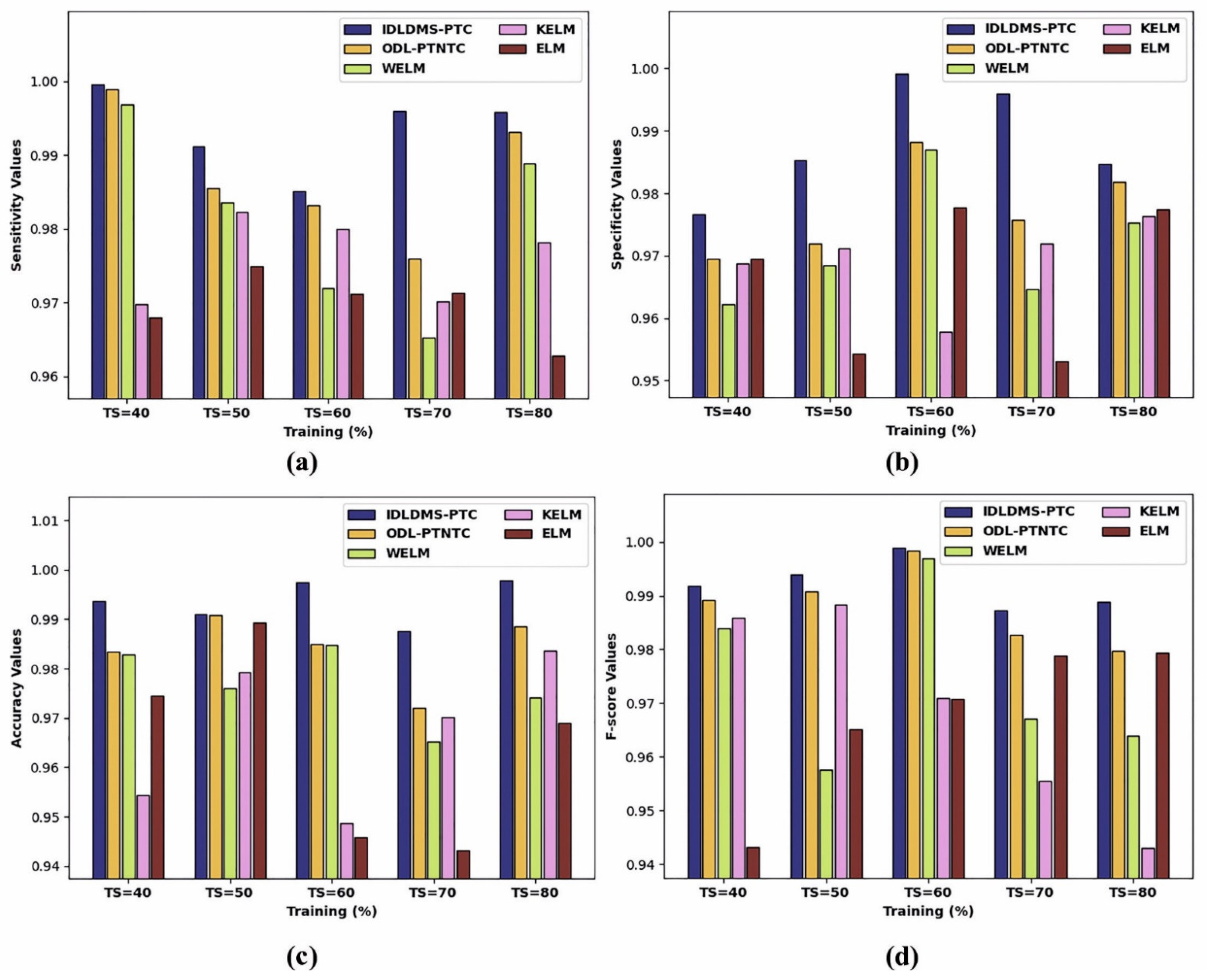
| Training (%) | IDLDMS-PTC | ODL-PTNTC | WELM | KELM | ELM |
|---|---|---|---|---|---|
| Sensitivity | |||||
| TS = 40 | 0.9995 | 0.9989 | 0.9969 | 0.9697 | 0.9679 |
| TS = 50 | 0.9912 | 0.9855 | 0.9835 | 0.9823 | 0.9749 |
| TS = 60 | 0.9851 | 0.9832 | 0.9720 | 0.9800 | 0.9712 |
| TS = 70 | 0.9960 | 0.9759 | 0.9653 | 0.9702 | 0.9713 |
| TS = 80 | 0.9958 | 0.9931 | 0.9889 | 0.9782 | 0.9628 |
| Average | 0.9935 | 0.9873 | 0.9813 | 0.9761 | 0.9696 |
| Specificity | |||||
| TS = 40 | 0.9767 | 0.9696 | 0.9622 | 0.9687 | 0.9696 |
| TS = 50 | 0.9853 | 0.9720 | 0.9684 | 0.9712 | 0.9543 |
| TS = 60 | 0.9992 | 0.9882 | 0.9870 | 0.9578 | 0.9778 |
| TS = 70 | 0.9959 | 0.9757 | 0.9646 | 0.9719 | 0.9531 |
| TS = 80 | 0.9847 | 0.9818 | 0.9753 | 0.9764 | 0.9774 |
| Average | 0.9884 | 0.9775 | 0.9715 | 0.9692 | 0.9664 |
| Accuracy | |||||
| TS = 40 | 0.9937 | 0.9834 | 0.9829 | 0.9544 | 0.9746 |
| TS = 50 | 0.9911 | 0.9908 | 0.9760 | 0.9792 | 0.9893 |
| TS = 60 | 0.9974 | 0.9850 | 0.9847 | 0.9487 | 0.9459 |
| TS = 70 | 0.9876 | 0.9721 | 0.9652 | 0.9702 | 0.9432 |
| TS = 80 | 0.9978 | 0.9886 | 0.9742 | 0.9837 | 0.9690 |
| Average | 0.9935 | 0.9840 | 0.9766 | 0.9672 | 0.9644 |
| F-score | |||||
| TS = 40 | 0.9919 | 0.9892 | 0.9839 | 0.9859 | 0.9432 |
| TS = 50 | 0.9940 | 0.9908 | 0.9576 | 0.9884 | 0.9651 |
| TS = 60 | 0.9989 | 0.9984 | 0.9970 | 0.9710 | 0.9708 |
| TS = 70 | 0.9873 | 0.9827 | 0.9671 | 0.9555 | 0.9788 |
| TS = 80 | 0.9889 | 0.9798 | 0.9640 | 0.9431 | 0.9793 |
| Average | 0.9948 | 0.9882 | 0.9739 | 0.9688 | 0.9674 |
| No. of Folds | IDLDMS-PTC | ODL-PTNTC | WELM | KELM | ELM |
|---|---|---|---|---|---|
| Sensitivity | |||||
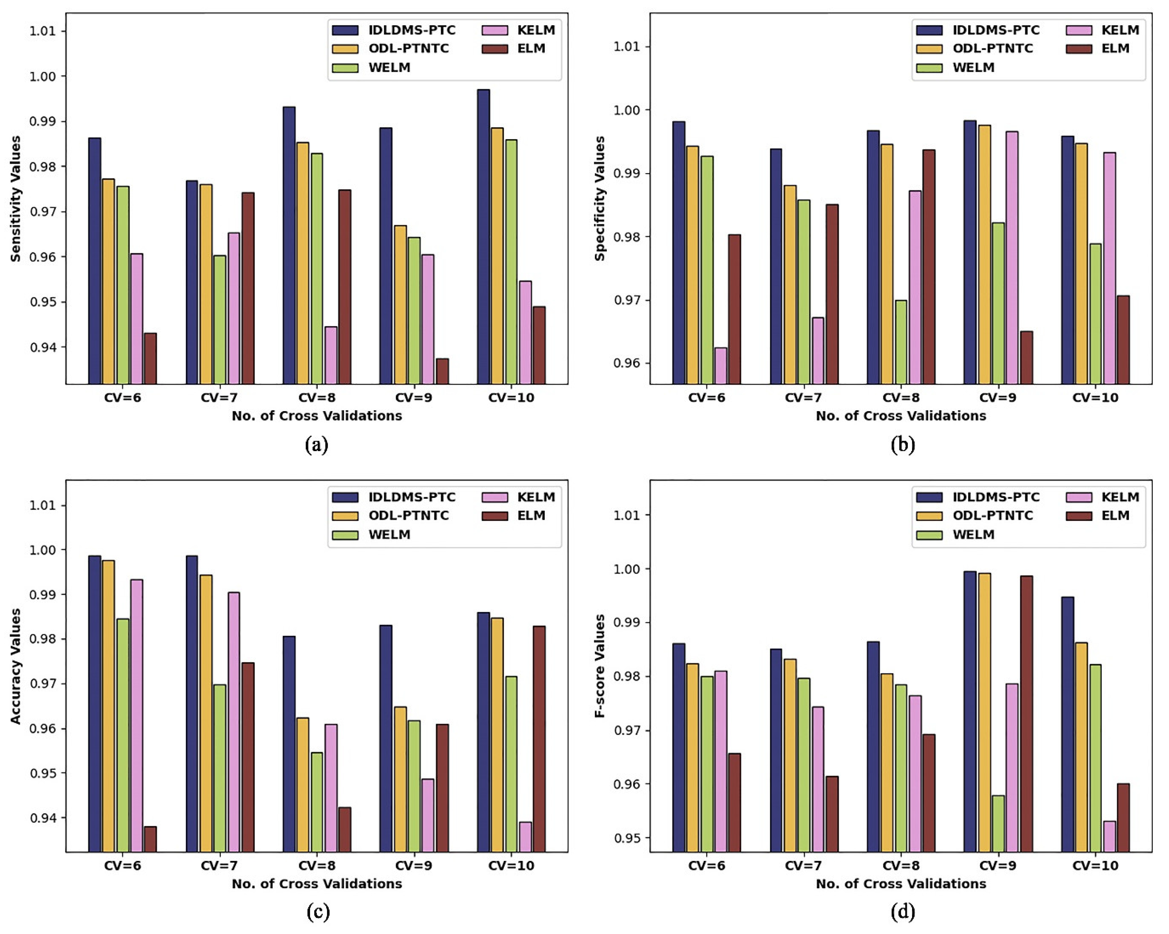
| CV=6 | 0.9864 | 0.9773 | 0.9757 | 0.9607 | 0.9431 |
| CV=7 | 0.9768 | 0.9761 | 0.9603 | 0.9654 | 0.9741 |
| CV=8 | 0.9931 | 0.9853 | 0.9829 | 0.9445 | 0.9748 |
| CV=9 | 0.9885 | 0.9670 | 0.9644 | 0.9605 | 0.9375 |
| CV=10 | 0.9970 | 0.9885 | 0.9859 | 0.9546 | 0.9489 |
| Average | 0.9884 | 0.9788 | 0.9738 | 0.9571 | 0.9557 |
| Specificity | |||||
| CV = 6 | 0.9981 | 0.9942 | 0.9927 | 0.9625 | 0.9803 |
| CV = 7 | 0.9938 | 0.9880 | 0.9857 | 0.9672 | 0.9851 |
| CV = 8 | 0.9967 | 0.9945 | 0.9699 | 0.9872 | 0.9937 |
| CV = 9 | 0.9983 | 0.9975 | 0.9822 | 0.9965 | 0.9650 |
| CV = 10 | 0.9958 | 0.9947 | 0.9788 | 0.9932 | 0.9706 |
| Average | 0.9965 | 0.9938 | 0.9819 | 0.9813 | 0.9789 |
| Accuracy | |||||
| CV = 6 | 0.9986 | 0.9977 | 0.9846 | 0.9934 | 0.9379 |
| CV = 7 | 0.9987 | 0.9944 | 0.9698 | 0.9904 | 0.9746 |
| CV = 8 | 0.9807 | 0.9623 | 0.9546 | 0.9610 | 0.9422 |
| CV = 9 | 0.9831 | 0.9648 | 0.9618 | 0.9486 | 0.9609 |
| CV = 10 | 0.9860 | 0.9847 | 0.9715 | 0.9389 | 0.9829 |
| Average | 0.9894 | 0.9808 | 0.9685 | 0.9665 | 0.9597 |
| F-score | |||||
| CV = 6 | 0.9861 | 0.9824 | 0.9799 | 0.9810 | 0.9657 |
| CV = 7 | 0.9850 | 0.9832 | 0.9796 | 0.9744 | 0.9615 |
| CV = 8 | 0.9864 | 0.9805 | 0.9784 | 0.9764 | 0.9692 |
| CV = 9 | 0.9995 | 0.9992 | 0.9578 | 0.9786 | 0.9987 |
| CV = 10 | 0.9948 | 0.9863 | 0.9821 | 0.9531 | 0.9600 |
| Average | 0.9904 | 0.9863 | 0.9756 | 0.9727 | 0.9710 |
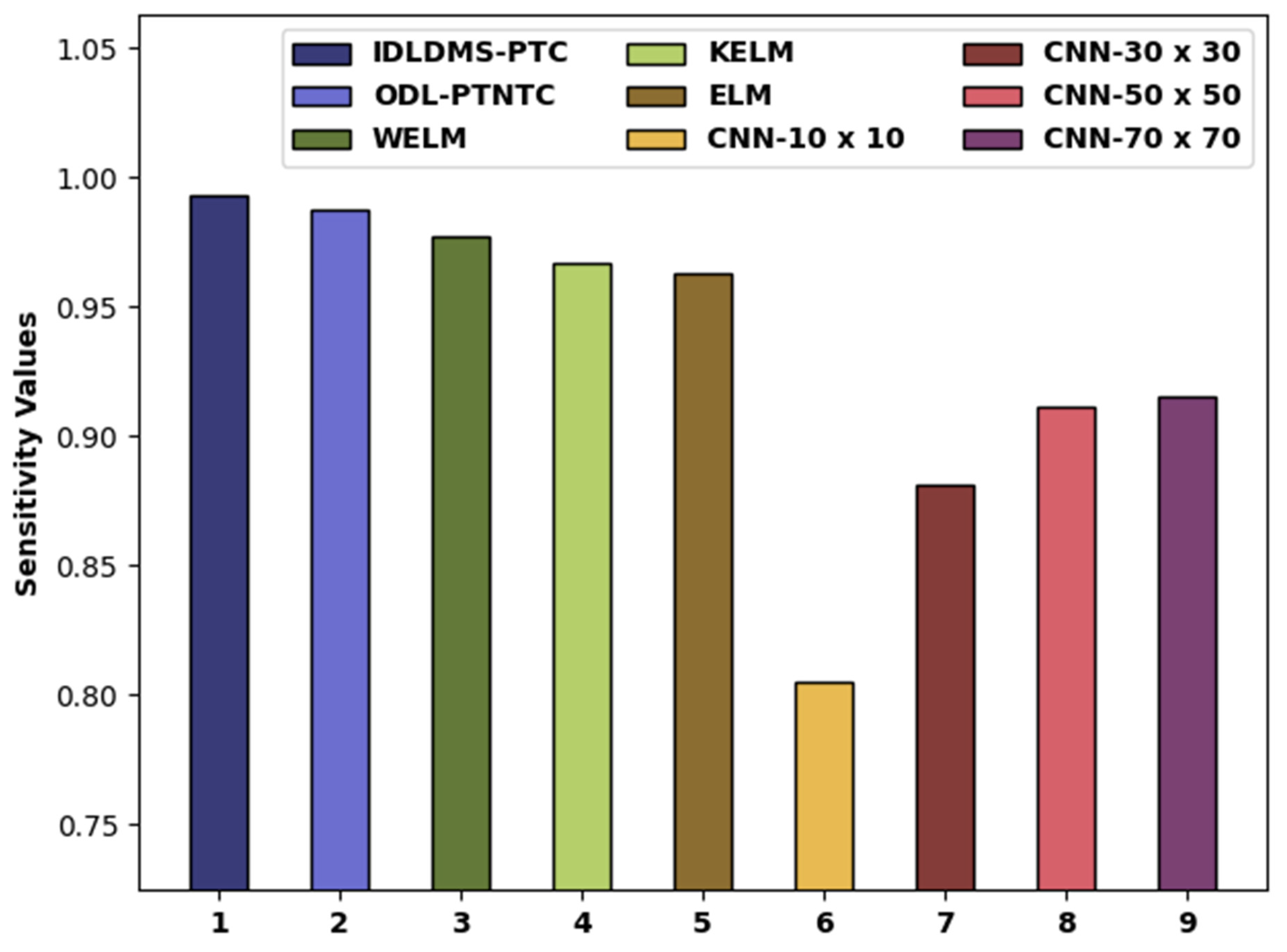
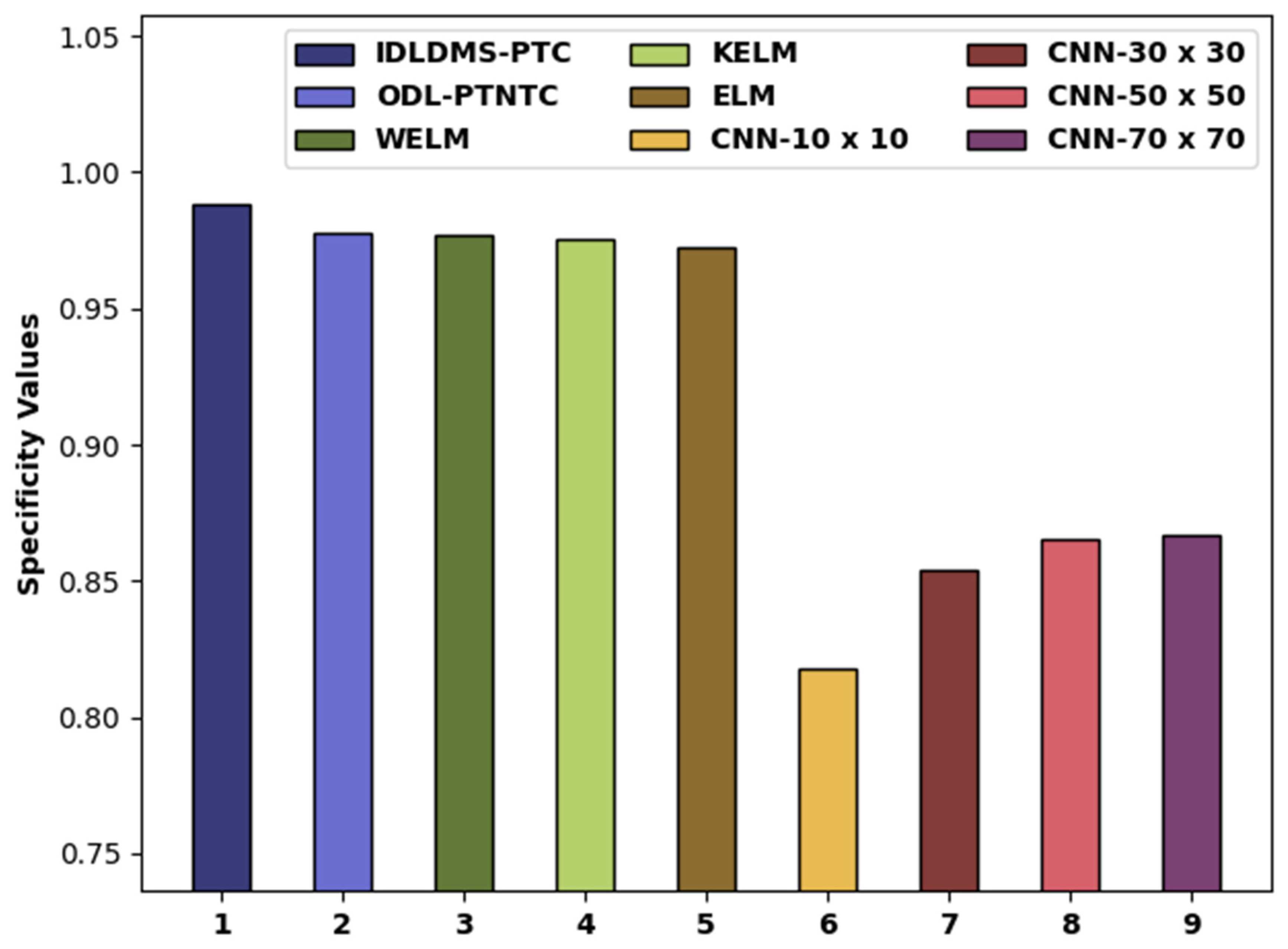
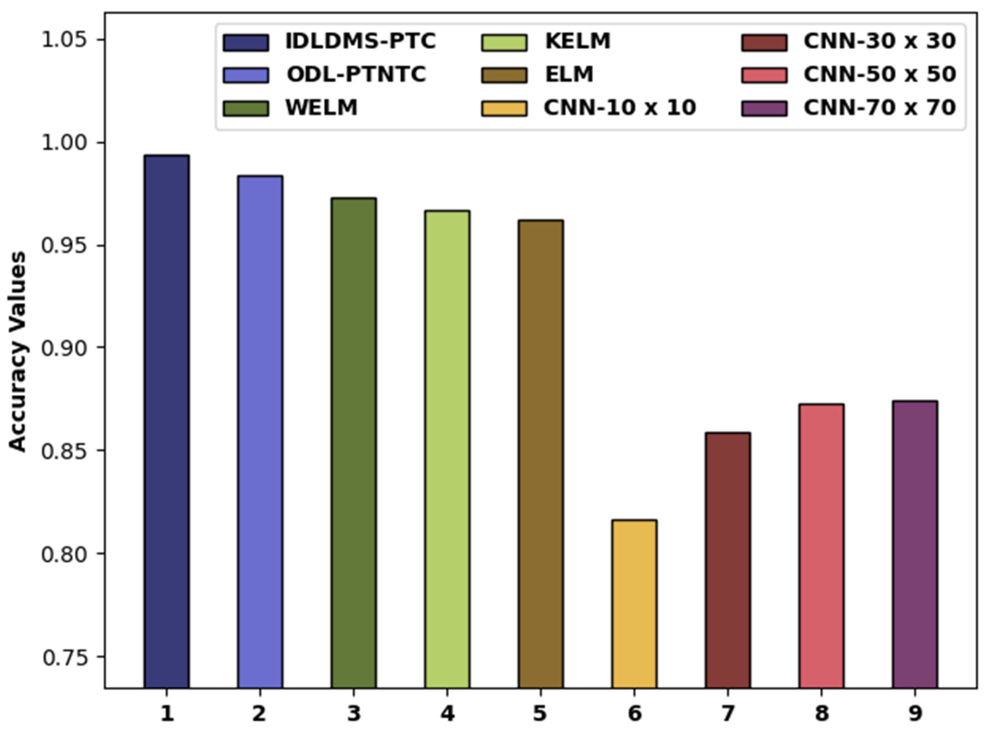
| Methods | Sensitivity | Specificity | Accuracy |
|---|---|---|---|
| IDLDMS-PTC | 0.9935 | 0.9884 | 0.9935 |
| ODL-PTNTC | 0.9873 | 0.9775 | 0.9840 |
| WELM | 0.9776 | 0.9767 | 0.9726 |
| KELM | 0.9666 | 0.9753 | 0.9669 |
| ELM | 0.9627 | 0.9727 | 0.9621 |
| CNN-10x10 | 0.8050 | 0.8180 | 0.8160 |
| CNN-30x30 | 0.8810 | 0.8540 | 0.8590 |
| CNN-50x50 | 0.9110 | 0.8650 | 0.8730 |
| CNN-70x70 | 0.9150 | 0.8670 | 0.8740 |
Publisher’s Note: MDPI stays neutral with regard to jurisdictional claims in published maps and institutional affiliations. |
© 2022 by the authors. Licensee MDPI, Basel, Switzerland. This article is an open access article distributed under the terms and conditions of the Creative Commons Attribution (CC BY) license (https://creativecommons.org/licenses/by/4.0/).
Share and Cite
Vaiyapuri, T.; Dutta, A.K.; Punithavathi, I.S.H.; Duraipandy, P.; Alotaibi, S.S.; Alsolai, H.; Mohamed, A.; Mahgoub, H. Intelligent Deep-Learning-Enabled Decision-Making Medical System for Pancreatic Tumor Classification on CT Images. Healthcare 2022, 10, 677. https://doi.org/10.3390/healthcare10040677
Vaiyapuri T, Dutta AK, Punithavathi ISH, Duraipandy P, Alotaibi SS, Alsolai H, Mohamed A, Mahgoub H. Intelligent Deep-Learning-Enabled Decision-Making Medical System for Pancreatic Tumor Classification on CT Images. Healthcare. 2022; 10(4):677. https://doi.org/10.3390/healthcare10040677
Chicago/Turabian StyleVaiyapuri, Thavavel, Ashit Kumar Dutta, I. S. Hephzi Punithavathi, P. Duraipandy, Saud S. Alotaibi, Hadeel Alsolai, Abdullah Mohamed, and Hany Mahgoub. 2022. "Intelligent Deep-Learning-Enabled Decision-Making Medical System for Pancreatic Tumor Classification on CT Images" Healthcare 10, no. 4: 677. https://doi.org/10.3390/healthcare10040677