
Robust Mode Analysis


1
Department of Physics, University of Houston, Houston, TX 77204, USA
2
Spectral Energies, LLC, Dayton, OH 45431, USA
*
Authors to whom correspondence should be addressed.
†
Both authors contributed equally to this work.
Mathematics 2021, 9(9), 1057; https://doi.org/10.3390/math9091057
Submission received: 7 April 2021
/
Revised: 27 April 2021
/
Accepted: 1 May 2021
/
Published: 8 May 2021
(This article belongs to the Special Issue Dynamical Systems and Operator Theory)
Abstract
:In this paper, we introduce a model-free algorithm, robust mode analysis (RMA), to extract primary constituents in a fluid or reacting flow directly from high-frequency, high-resolution experimental data. It is expected to be particularly useful in studying strongly driven flows, where nonlinearities can induce chaotic and irregular dynamics. The lack of precise governing equations and the absence of symmetries or other simplifying constraints in realistic configurations preclude the derivation of analytical solutions for these systems; the presence of flow structures over a wide range of scales handicaps finding their numerical solutions. Thus, the need for direct analysis of experimental data is reinforced. RMA is predicated on the assumption that primary flow constituents are common in multiple, nominally identical realizations of an experiment. Their search relies on the identification of common dynamic modes in the experiments, the commonality established via proximity of the eigenvalues and eigenfunctions. Robust flow constituents are then constructed by combining common dynamic modes that flow at the same rate. We illustrate RMA using reacting flows behind a symmetric bluff body. Two robust constituents, whose signatures resemble symmetric and von Karman vortex shedding, are identified. It is shown how RMA can be implemented via extended dynamic mode decomposition in flow configurations interrogated with a small number of time-series. This approach may prove useful in analyzing changes in flow patterns in engines and propulsion systems equipped with sturdy arrays of pressure transducers or thermocouples. Finally, an analysis of high Reynolds number jet flows suggests that tests of statistical characterizations in turbulent flows may best be done using non-robust components of the flow.
1. Introduction
It is rarely known at sufficient detail that the operation of many technologically important processes relying on strongly driven fluid or reacting flows can be controlled or optimized through modeling. For example, due to chamber feedback and unsteady heat release [1,2], it is difficult to establish a priori how the fuel efficiency and power output of airplane engines or efficacy of industrial reactors can be enhanced while maintaining their integrity. Attempts to reduce the fuel/air ratio in an airplane engine can cause flame extinction [3]; strong driving of industrial reactors can initiate highly damaging, and spontaneously forming “hot spots” [4]. The ability to establish the nature of such flows and identify their changes can aid in design improvements to control or suppress undesirable facets of the flows. Such an approach is outlined here.
A major difficulty in control is incomplete knowledge of the underlying systems [1]. Although the Navier-Stokes equations modeling fluid flows are known [5,6,7,8], reaction-diffusion systems for combustion are typically only known approximately. Even in rare instances when the underlying dynamics are known, the absence of symmetries or other simplifying constraints in realistic configurations preclude the derivation of solutions. Difficulties can originate from nonlinearity of the underlying equations and the resulting sensitive dependence on initial conditions, as well as the preponderance of nonlinearly coupled flow constituents that permeate strongly driven flows [9]. The emergence of structures, such as eddies and vortices, over a wide range of temporal and spatial scales complicates numerical integration of the underlying systems as well.
Experimental studies of reacting flows have seen significant advancements through recent developments in experimental techniques, such as particle-image-velocimetry (PIV), planar laser-induced fluorescence (PLIF), and high-resolution chemiluminescence. In PIV, the flow is seeded with light tracer particles, which are imaged to deduce flow velocity fields [10,11]. In PLIF, light illuminates a medium which fluoresces; this signal is captured by a detector and inverted to yield quantitative characteristics of the medium [12]. Chemiluminescence uses light emission from atoms or molecules to establish the location and density of products in reacting flows [13]. These techniques permit high-frequency, high-resolution measurements of velocity, density, and temperature fields in a flow. The question then is how flow characteristics can be extracted directly from experimental data.
One difficulty that emerges in such studies involves differentiating flow dynamics from “noise”, by which we mean the content in the signal not directly inferred from the underlying dynamical system. Examples of noise include measurement errors, unaccounted long-range interactions, slow variations in the baseline due to changes (e.g., temperature) in the experimental or laboratory set-up, and so forth. In addition, the near-translational invariance of large systems introduces “slosh dynamics” [14], that is, low-frequency movements of the baseline. Typically, it is not known how such irregular facets can be accounted for and eliminated from an experimental signal. In strongly-driven fluid and combustion flows, their effects are compounded by nonlinearity, and the consequent sensitive-dependence on initial conditions [9]. A priori, it is not clear how coupling between dynamical modes, between dynamical modes and extraneous ones, or facets like measurement errors can be dissociated.
The standard approach to analyzing fluid or combustion flows is its interpretation as the collective evolution of a set of “coherent structures” , whereby the dynamics of a flow field is decomposed as
The most widely-used class of coherent structures is derived through proper orthogonal decomposition (POD) [15,16,17,18,19]. They are eigenfunctions of the matrix of pair-wise correlations of the field at different sites, arranged in decreasing order of their contribution to variations in the field. POD gives the most “efficient” decomposition in the sense that at any level of truncation, no other class of coherent structures captures a larger fraction of variations [16]. Typically, dynamics of ’s are coupled due to nonlinearity of the underlying system.
A second class of coherent structures is given by dynamic mode decomposition (DMD) [20,21,22,23,24]. A dynamic mode is a spatial structure that oscillates at a fixed (complex) frequency; that is, the coefficients in Equation (1) evolve as , for . The spatio-temporal flow dynamics can be interpreted as the sum of oscillating dynamic modes. Under appropriate conditions, DMD is a form of Koopman mode analysis, originally constructed to explain the linearity of quantum mechanics even for classically nonlinear systems [22,23,24,25,26,27]. Unlike for POD modes, the evolution of a dynamic mode is independent of the others. In addition, dynamic modes are a natural class of coherent structures to expand flows containing, for example, periodic vortex shedding.
DMD offers means to partially address the question posed earlier on delineating flow dynamics from noise and other irregular facets. As in Fourier expansion of a noisy signal, DMD expands all facets of the signal , including noise, in periodically evolving modes. The question then is which of these modes represent dynamical features of the flow. Robust mode analysis (RMA) identifies them as dynamic modes common to multiple, nominally identical, experimental realizations; the commonality is established through proximity of the dynamic modes and the associated eigenvalues. The dynamic mode decomposition and implementation of RMA are outlined in Section 2.
RMA differs from robust principal components analysis (RPCA), whose intent is to partition a spatio-temporal field into a low-rank constituent and one that consists of a collection of “sparse” modes [28,29]. RPCA can, for example, separate rapid changes in a traffic pattern from a slow varying background. In contrast, RMA does not require differences in time-scales or “energy content” to differentiate robust and non-robust features. We will show through examples that robust modes are not necessarily those with the highest energy.
Three applications of RMA are given in Section 3, Section 4 and Section 5. Section 3 analyzes PLIF data from an experiment in a reacting flow past a single symmetric bluff body. At sufficiently high Reynolds numbers, bluff-body flows exhibit symmetric vortex shedding, where pairs of vortices are shed periodically from either side simultaneously [3]. In lean mixtures, the flow also exhibits von Karman vortex shedding, where vortices are shed periodically from alternate sides of the bluff body [30]. RMA yields a collection of robust dynamic modes, which can be grouped by comparing downstream flow rates. The two classes so derived are found to be symmetric and von Karman vortex shedding. The results in Section 3 were adapted from the Ref. [31].
Section 4 re-analyzes reacting flows behind a single symmetric bluff body, now using time-series from a small number of transducers, rather than through spatio-temporal fields. Such analyses can prove important in following, for example, changes in flow patterns within airplane engines or in industrial scale reactors. Their failure is often caused by the (slow) progression of domains with micro-cracks or material degradation. Changes in flow patterns may precede catastrophic failure. In contrast to PIV or PLIF which require robust optical access, time-series measurements can be made continuously, since most engines and propulsion systems are equipped with sturdy arrays of pressure transducers and thermocouples. The analysis requires “enhancing” the spatial field using extended DMD [24,27], which in this application, is made using Chebyshev polynomials. RMA, implemented on the extended field, once again, yields one robust mode in rich mixtures and two in lean mixtures. Time-series of projections of the first to pairs of symmetrically-placed transducers can be used to infer that it is up-down symmetric (justifying its association with symmetric vortex shedding), while the second is not (von Karman shedding).
The final application presented in Section 5 involves turbulent jet flows which are quantified using statistical properties of the flow. The experimental data consist of high-resolution, high-frequency (100 kHz), two-dimensional velocity fields in a plane of symmetry. The flow data can be used to extract distributions of single-point fluctuations (which are empirically found to be nearly Gaussian) and the variance-covariance matrix for velocity fluctuations at two sites. Moments of structure functions between two points are derived from this observation. The experimental flow fields are likely to be corrupted by perturbations, such as acoustic reflections from the laboratory walls that are not included in an analysis. We assume that perturbations extraneous to the experimental setup can be identified through RMA. The remaining flow fields are those whose statistics should be compared with predictions. In fact, we are able to show that structure functions of the non-robust velocity fields more closely follow the computed one than the original flow.
Section 6 summarizes some implications of our findings.
2. Dynamic Mode Decomposition and Robust Mode Analysis
2.1. Dynamic Mode Decomposition
Dynamic mode decomposition (DMD) [20,21,22,24] provides a class of coherent structures. In contrast to POD, which categorizes coherent structures according to correlations, DMD assorts them through spatial structures that oscillate with a single (complex) frequency. Hence, it is a natural approach to extract periodic flow constituents, such as symmetric or von Karman vortex shedding. In addition, DMD has a theoretical basis in the Koopman operator theory [23,24,25], and the dynamics of the modes are decoupled from each other.
We provide a summary of DMD: suppose spatio-temporal dynamics of a field at time-step n is expressed as , being a field recorded at site and the entire “snapshot” is recorded at discrete time-points . The primary conjecture in DMD is that the operation to transform from to is independent of the “initial” state , and hence that a sufficiently large number of snapshots can be used to find properties of the underlying dynamics. (Note that snapshots obtained during a transition between two states far-away in state space may not satisfy the requirement.) Under the assumption, when snapshots are recorded at sufficiently short uniform time-intervals (so linear expansion suffices), we could write
where is a representation of the flow dynamics within the duration . When N is sufficiently large, singular value decomposition is used to find the spectrum of . The coherent structures (dynamic modes) are the eigen-vectors , which evolve as , (the generally complex) being the associated eigenvalue. Thus, each dynamic mode evolves periodically with a period . The field can be expanded in dynamic modes [20,21,22,24].
2.2. Robust Mode Analysis
Robust mode analysis (RMA) uses dynamic modes (1) to differentiate dynamical features of a flow from noise and other irregular facets, and (2) to identify flow constituents. Here, as in POD or Fourier analysis of a time-series, noise and other irregular (e.g., initial-condition differences amplified by sensitive dependence on initial conditions) features contribute to DMD as well. RMA is predicated on the expectation that while dynamical features of the flow will retain their form (i.e., dynamic modes and eigenvalues, although not necessarily the intensity) in different realizations of an experiment, irregular features will differ between experiments. Under this scenario, robust flow modes are those common to multiple realizations of an experiment.
To be specific, denote the dynamic modes and eigenvalues for the first experiment by , and those of the next set of experiments by . Dynamic modes from the different groups are assumed to be the same if they satisfy the following criteria:
- Imaginary parts of the eigenvalues from multiple groups should be sufficiently close; specifically,where is a cutoff.
- The real parts of an eigenvalue identified from the first condition should not vary significantly among the subgroups; specifically,for a cutoff . For work reported here, we limit consideration to .
- Dynamic modes from the different groupings that satisfy Equations (3) and (4) should be close. Specifically, if and are normalized eigenfunctions associated with proximate eigenvalues, thenfor a cutoff . The minimization over the phase is implemented to account for the fact that eigenfunctions computed from different experimental realizations may differ in phase.
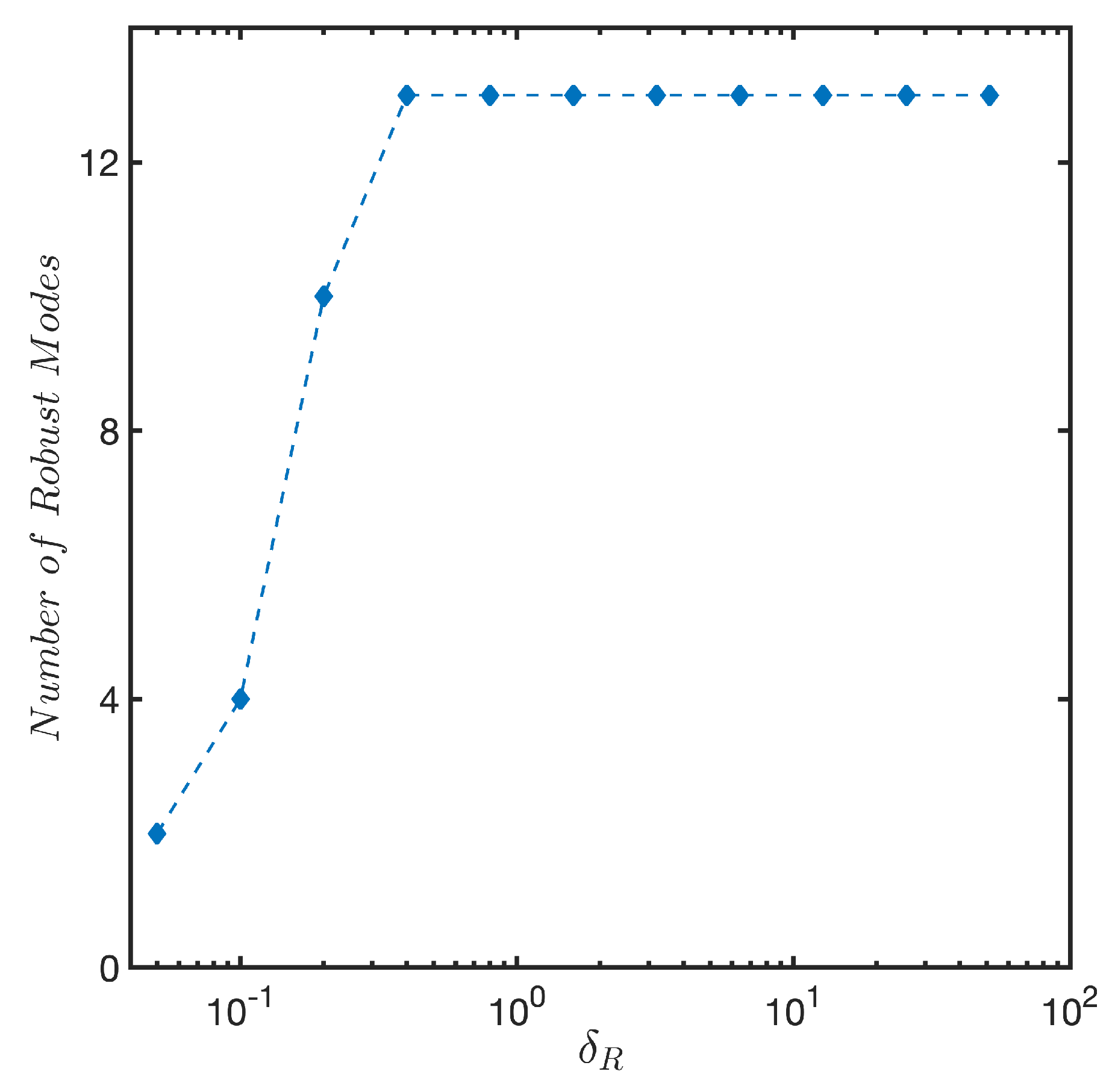
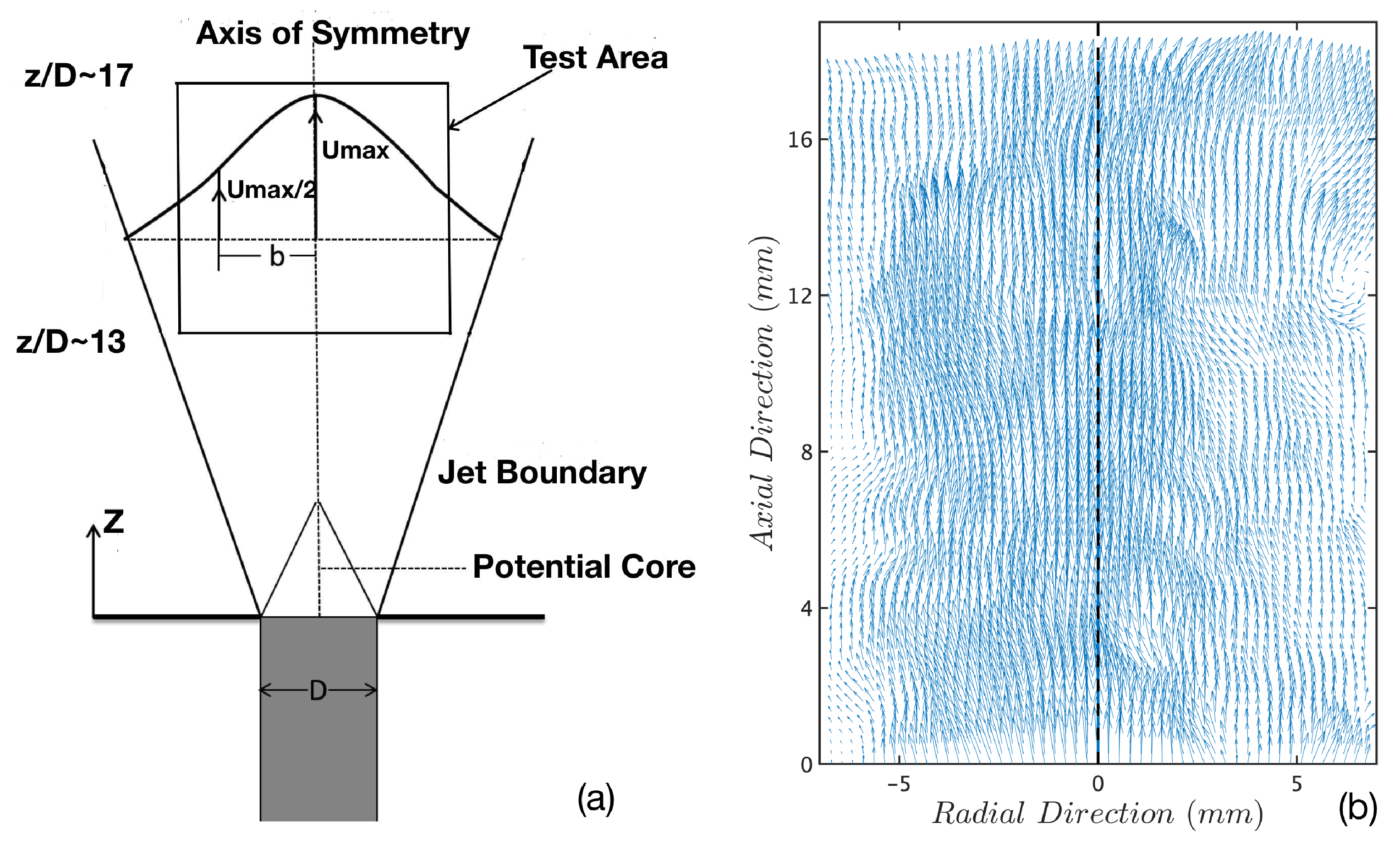
Robust mode analysis is conducted on the entire spatial field, which is typically a few thousand measurements. The cutoff values , , and depend on properties of an experimental system, including the level of noise, and need to be established heuristically. We limit consideration to in order to restrict the parameter search. We illustrate the selection of the cutoff values using spatio-temporal flow fields in a turbulent jet flow of Reynold’s number 21,000, described in Section 5. The data consist of axial and radial velocity fields on a lattice of size at a rate of 100 kHz for a duration 0.08 s.
We note first that for unit vectors and , . Furthermore, the probability density function for the angle between two random vectors in N dimensions satisfies . Thus, for sufficiently smaller than , the likelihood of the left side of the last inequality being satisfied with no underlying reason is minuscule. For fixed , we search for robust modes beginning with a small (say ), and ascertain increases in their number with increasing . There is a proliferation of robust modes outside the Nyquist range (i.e., ) when increases beyond ∼0.85. Furthermore, no new robust modes appear in , motivating the choice of . Next, we compute how the number of robust modes increases with ; this is shown in Figure 1. These considerations suggest that there are 13 robust modes in the jet flow, three of which have real ’s.
We studied the effect of noise on the choice of , , and by adding synthetic Gaussian “noise” to the experimental data. The magnitude of the synthetic noise was quantified using a measure of the inverse of the signal-to-noise ratio , defined as the ratio of the standard deviation of the Gaussian noise to that of the field. As increases beyond ∼0.3, the number of robust modes is found to decrease. The remaining modes can be associated with those for the noise-free case through proximity of the eigenvalues. In addition, some (although not all) of the robust modes lost on adding noise can be recovered by increasing .
Note that cutoffs , , and do not depend on the (mean) magnitude of the experimental data fields. Since the eigenfunctions are normalized, the difference in phases is independent of the magnitude. In addition, since the eigenvalues of the matrix are expressed as , the imaginary parts do not depend on the magnitude as well. Although the real parts do depend on the mean magnitude, differences between pairs of eigenvalues from different experiments are independent of the scale.
RMA is best used on data from a group of distinct experiments. However, we have used the following approach in cases where only a single experimental recording is available. The full set of snapshots is assigned as Group 1. The remaining groups are constructed using (1) the first half of snapshots, (2) the second half of snapshots, (3) even-numbered snapshots, and (4) odd-numbered snapshots. We have established robust modes in combustion flow behind a bluff body [31], in axisymmetric injector flow [32], and swirling combustion flows [33] and found flow constituents consistent with prior studies. The analysis also uncovered a novel broken-symmetry mode in injector flows [32]. Although DMD is highly sensitive to noise and subsets of snapshots used for analysis [29,34,35], we find that imaginary parts of eigenvalues of robust modes in different sub-groupings typically do not change by more than a fraction of a percent.
We finally consider the construction of a robust flow constituent. As an example, a constituent may include a robust dynamic mode and its second harmonic, which itself may be robust. Our goal is to select robust modes that should be associated with the same flow constituent. For a given dynamic mode, we can use the evolution of the “phase” of the coefficient of Equation (1) (i.e., ) to quantify its motion. However, we note that the phase of the second harmonic will advance at twice the rate of that of the fundamental. In order to correct this difference, we note that geometric features of the harmonic, such as the number of local peaks, will also be twice that of the primary (as illustrated through examples in the Ref. [31]). Thus, we can associate a phase for each robust mode via
where is the number of local peaks in the dynamic mode. The “flow rate” of the robust mode is then defined as . With this definition, the fundamental and its harmonics will have the same flow rate. Once all robust modes with the same flow rate are identified, the associated flow constituent is reconstructed via
Applications in the use of the flow rate to construct flow constituents are given in the next section [31].
3. Reacting Flows behind a Single Bluff Body
3.1. The Experiment
Experiments were conducted within an optically accessible, atmospheric-pressure combustion test section that contains a bluff-body flame holder for flame stabilization. Air is delivered into a 152 mm mm rectangular test section at a constant rate of kg/s. While the air rate is maintained constant, propane fuel is added and mixed upstream of the flame holder, which is a v-gutter with a width of mm and an angle of 35. Additional facility details and flame-holder dimensions are provided in the Ref. [3].
The nature of instabilities in bluff-body flows depends on fractions of fuel and air in the mixture. It is quantified using the equivalence ratio defined as the fuel/air ratio of the mixture compared to that of its stoichiometric value (when all reactants are fully utilized). Fuel-rich mixtures are those with larger equivalence ratios, while lean mixtures are those with smaller equivalence ratios. In our configuration, flame blow-off occurs when and our experiments are performed for equivalence ratios between and . Symmetric vortex shedding [36,37] is observed in the entire range of , while the asymmetric von Karman vortices are only observed in a lean mixture () [3].
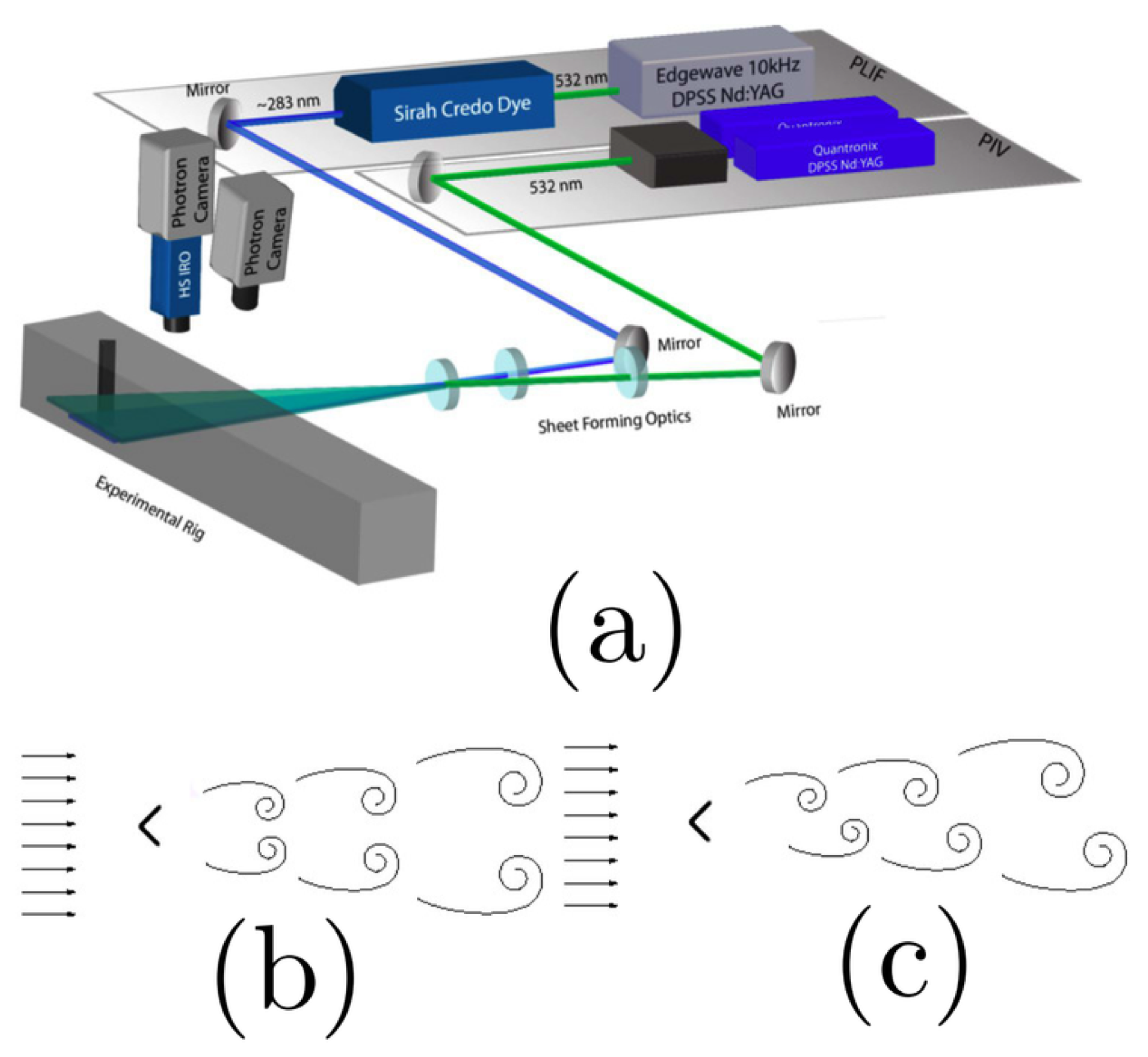
A schematic of the experimental setup is shown in Figure 2a [38], and two-dimensional images of hydroxyl (OH) behind the bluff-body v-gutter were acquired utilizing planar laser-induced fluorescence (PLIF), performed using a 10-kHz, diode-pumped, solid-state Nd:YAG laser and a tunable dye laser. The 532 nm output of the Edgewave laser was used to pump the dye laser for obtaining tunable laser output at ∼586 nm. This wavelength was then frequency-doubled at ∼283 nm to excite the rovibrational transition in the band of OH. The transition has a low Boltzmann-fraction sensitivity between temperatures of 1000 and 2400 K, minimizing the need for a temperature correction on Boltzmann distributions when extracting flame fronts. The PLIF signal of OH was collected employing a LaVision dual-stage, high-speed UV intensifier (IRO) coupled to a Photron SA-5 CMOS camera. The collected light was filtered using a Brightline Semrock filter with ∼90% transmission between 300 and 340 nm. Each recording contained 8000 frames separated by ms. Only the last 4000 frames were used for the DMD analysis.
Below, we summarize results from RMA on a flow at equivalence ratio , when both symmetric and von Kaman vortex shedding modes are active. These results were previously reported in the Ref. [31].
3.2. Results from Robust Mode Analysis
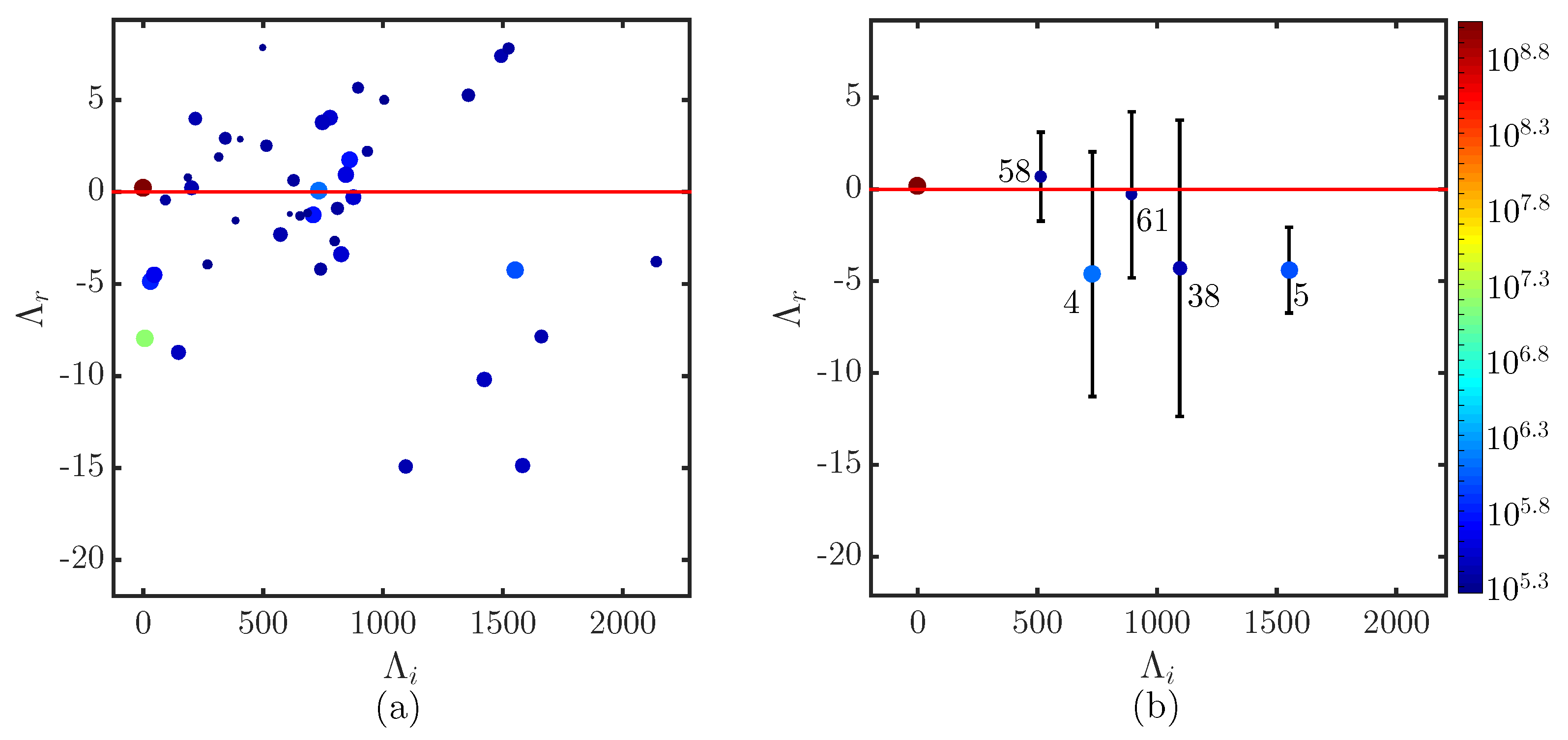
Figure 3a shows the eigenvalues of DMD modes and Figure 3b, those of the robust modes, which are identified using 2000-frame sections of the video. (Increasing the number of frames further introduces numerical errors in singular value decomposition, as can be inferred from emergence of a large number of eigenvalues with significantly different magnitudes from 1.) We compare dynamic modes from this full sequence with those from the first half, second half, odd-numbered snapshots, and even-numbered snapshots. The real parts of the robust modes vary between the subgroups and we show the mean and standard deviation for each robust mode. Note that the modes that remain past the decay of transients neither decay nor grow, and are thus expected to have zero real parts of their eigenvalues [22,23]; this is seen to be the case for the robust modes in Figure 3b. The mode numbers given in Figure 3b are ordered according to their energies.
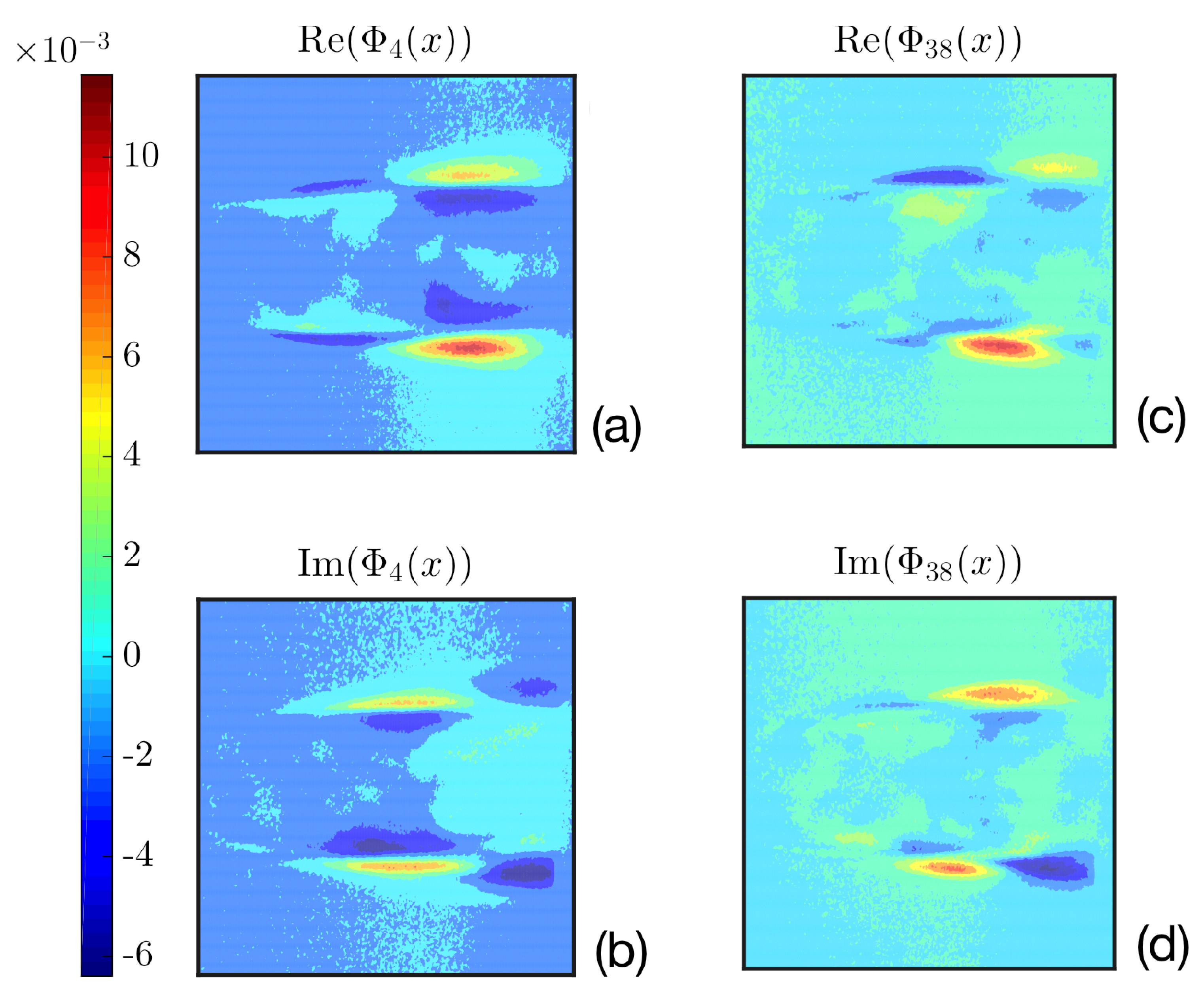
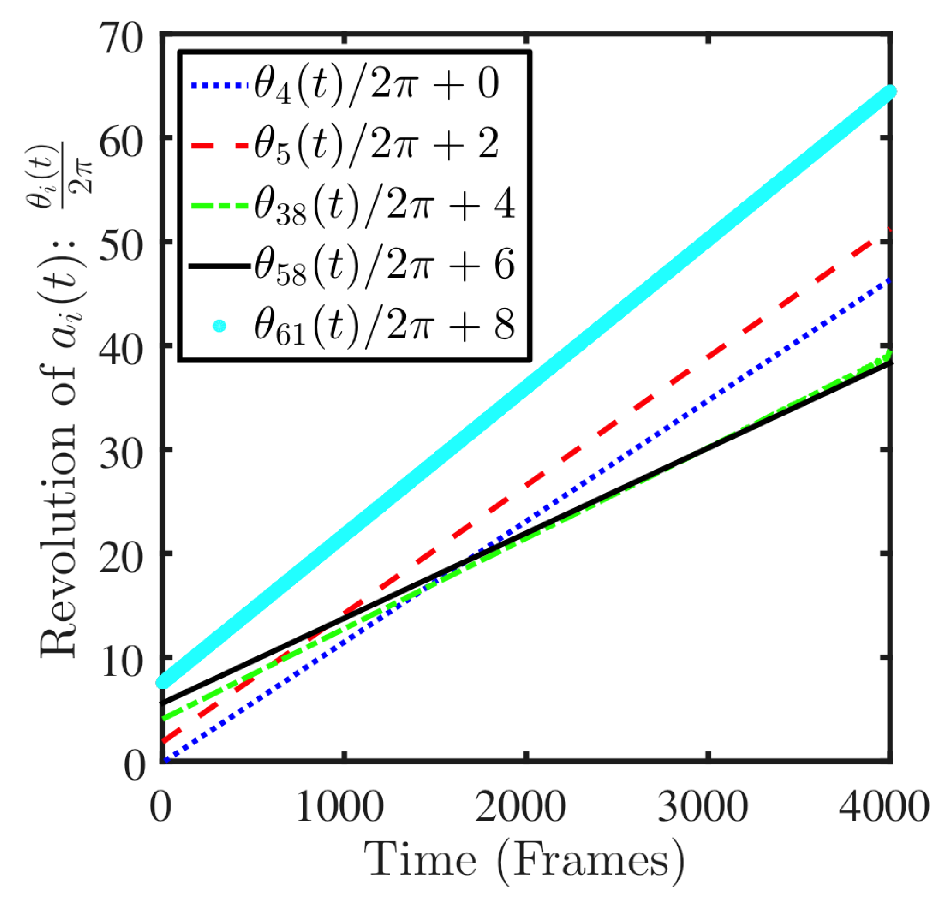
Robust modes 4 and 5 are symmetric about the x-axis, and modes 38 and 58 show a von Karman-like structure, as can be seen from Figure 4a,b, the real and imaginary parts of , and Figure 4c,d, the real and imaginary parts of .
The phase dynamics of these five modes are shown in Figure 5. The angular velocities and are approximately and radians/frame, respectively, suggesting that they belong to a single flow constituent. The angular velocities and are approximately 0.055 and 0.051 radians/frame, suggesting that they belong to a second flow constituent. However, the difference in angular velocities between the two pairs of modes (and the symmetry of the first pair and asymmetry of the second pair) implies that the two constituents are distinct. The reproduction of the dynamics of shows that the constituent represents von Karman vortex shedding. The difference between the downstream flow rates of the symmetric and von Karman vortices means that the overall shedding is not periodic.
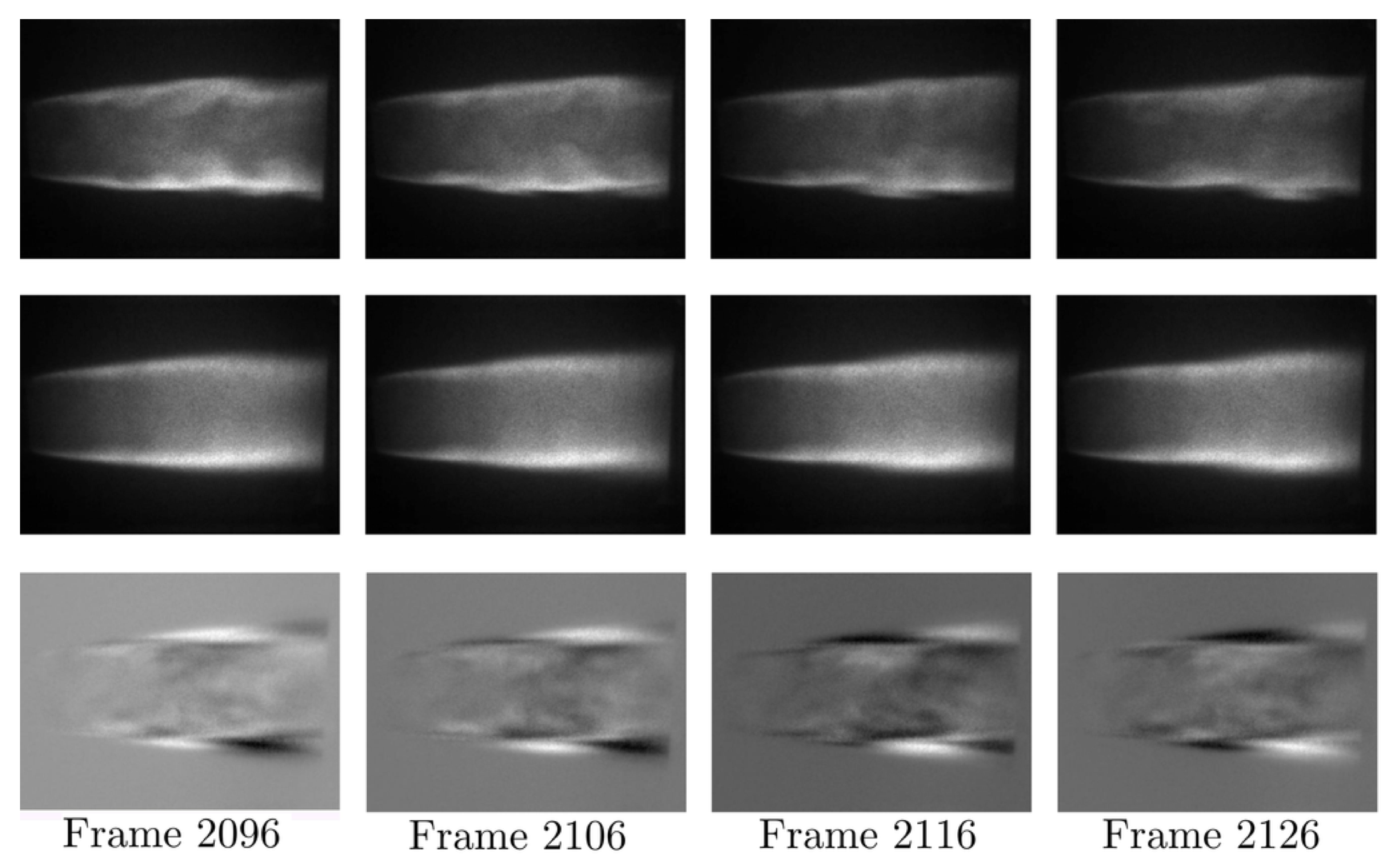
Finally, we present the reconstructions of the two flow constituents. The top row of Figure 6 contains several snapshots from the original flow. The next two rows show reconstructions of the symmetric and asymmetric constituents at the corresponding time-points. These can be interpreted as symmetric and von Karman vortex shedding. Here, evidence is found for the success of using DMD in separating the flow into distinct constituents. The symmetries of the constituents and the properties of their dynamics (for example, that the angular velocities are not identical) provide the information that is essential in the development of accurate low-dimensional models for the flow.
Mode 61 has a slightly higher angular velocity and appears less symmetric than modes 4 ad 5. For this work, we have chosen to not include it in the first flow constituent.
4. Bluff Body Flow Assessed by Discrete Devices: Extended DMD
Here, we once again implement RMA on combustion flows behind a symmetric bluff body, but using only pressure time-series from a small number of transducers. One of the key requirements in DMD is that the space of measurements are sufficiently large that eigenfunctions lie in their span. This is likely to fail when only measurements from a small number of transducers is all that is available. Consequently, a pre-processing step is implemented to extend [24,27,39] the “data-space”; we use Chebyshev polynomials of measurements at each transducer for the task. Robust modes computed from the analysis can be compared with those from Section 3 or derived from other approaches.
A broader goal belies these paradigmatic studies. Damage to engines or industrial reactors are often initiated by localized weakening of material (due to cyclic loading) through onset of microscopic fractures [40,41], which progress slowly until feedback-induced acceleration precipitates catastrophic failure. New flow patterns may be expected to emerge within a system prior to failure, and if so, techniques to identify them could provide predictive signatures of failure.
4.1. The Experiment
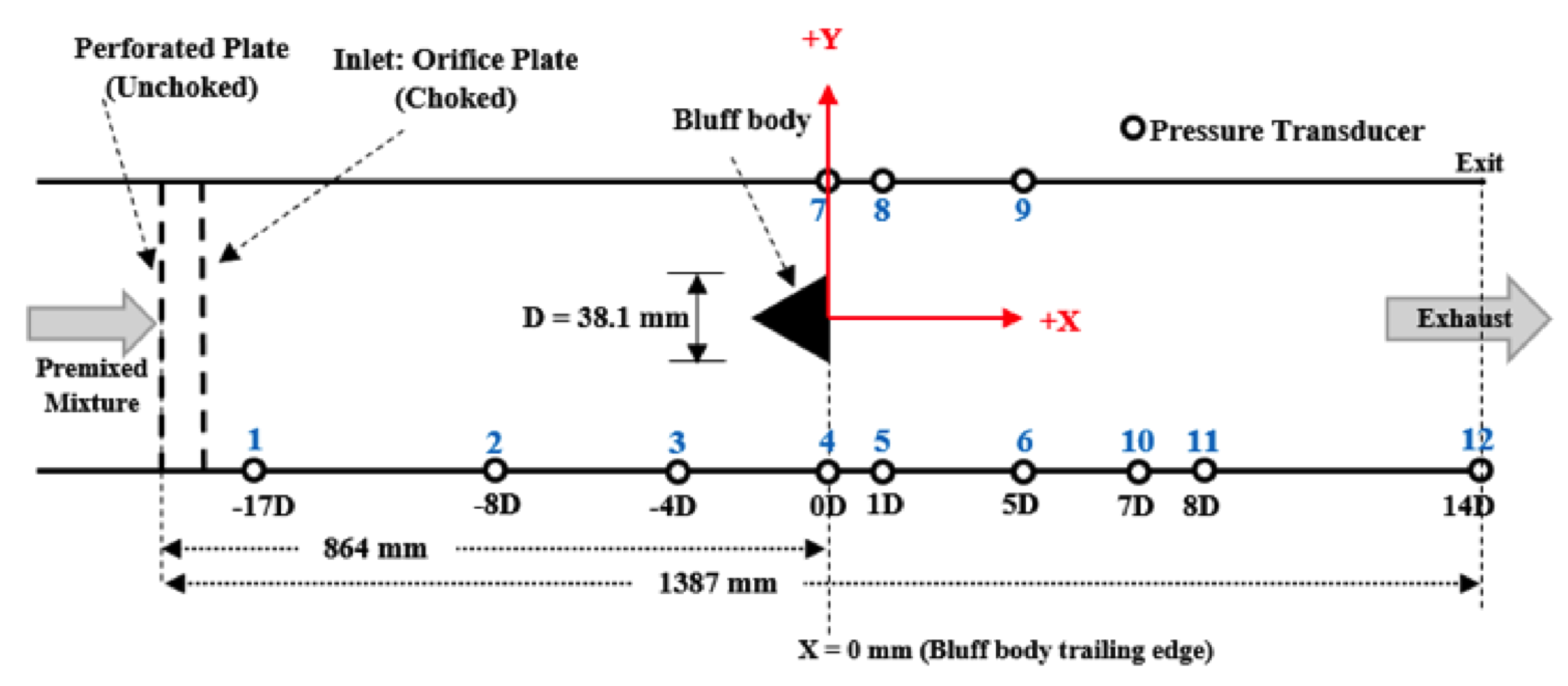
Here, measurements of the flow in the experimental arrangement described in Section 3.1 are made using a set of pressure transducers located on at , and at the exit on the bottom surface and at , and on the top surface, where mm is the width of the bluff body. Pressure measurements in each transducer were made for 20 s at a rate of 20 kHz. Figure 7 shows the arrangement schematically. The analysis below is for a combustion flow at of equivalence ratios , when only symmetric vortex shedding is observed, and at when both symmetric and von Karman shedding are observed.
4.2. Extended DMD and Robust Mode Analysis
Time-series from transducers 1–9 are “extended” synthetically using Chebyshev polynomials. The choice of Chebyshev polynomials is motivated by the fact that they provide finer temporal resolutions while remaining finite. Further, their use is computationally faster than the use of, for example, trigonometric functions. The number of polynomials used for the extension is made as follows: evaluate robust eigenvalues with increasing numbers of Chebyshev polynomials and search for convergence. For the bluff body data, the eigenvalues converge when the number is ∼8. We used 10 Chebyshev polynomials in our analysis. Such extensions, referred to as extended DMD, have been shown to successfully enhance the data space [24,27,39]; the spatial field is effectively enhanced to 90 sites. Robust mode analysis is implemented using five sub-intervals, each of 10,000 time steps (i.e., 500 ms), as distinct, nominally-identical experiments. Robust modes were identified using the criteria outlined before.
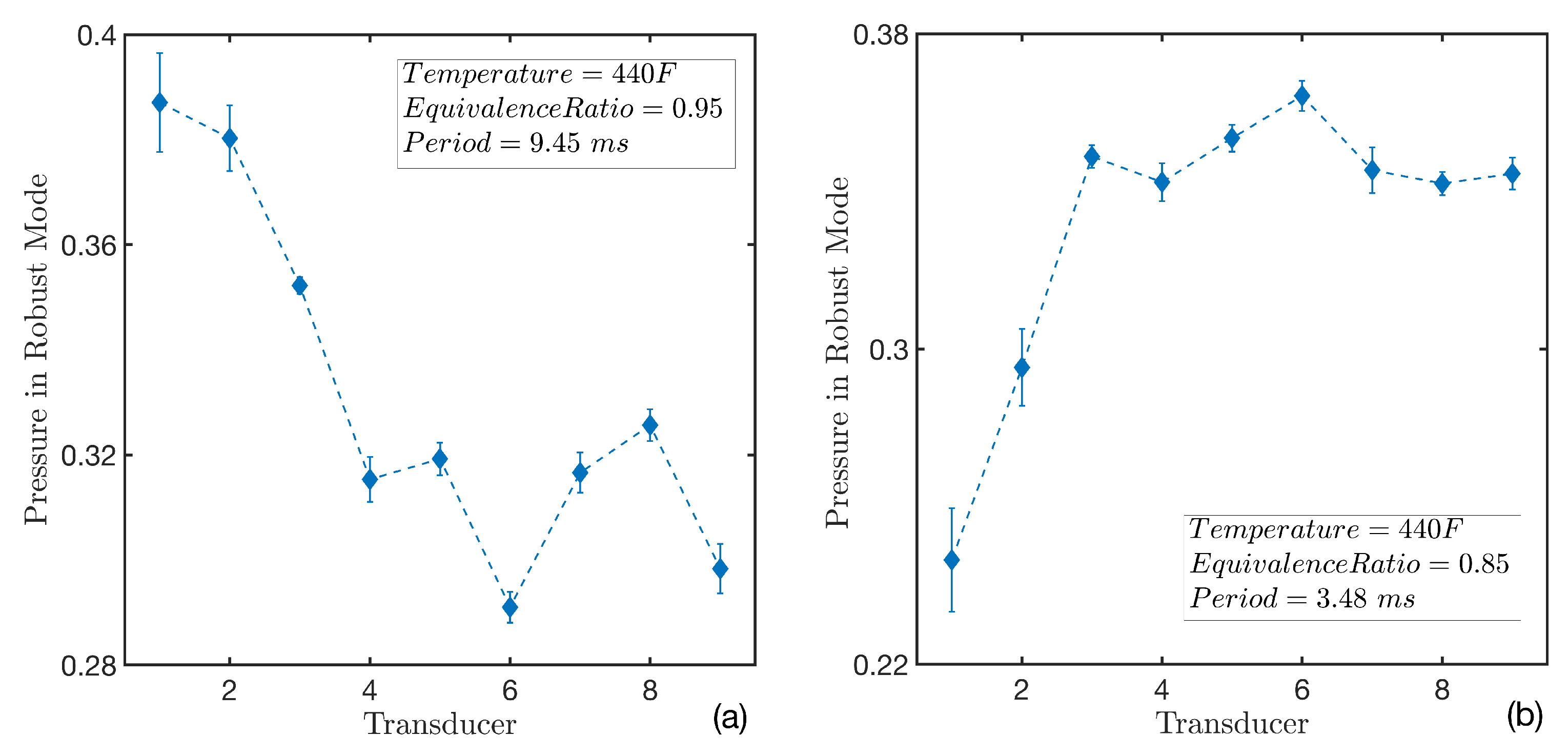
Only a single pair of robust modes and period ms, is found in the first experiment, at the equivalence ratio . Projections of the mean and the standard deviation of the robust mode to the space of the signals from the nine transducers are shown in Figure 8a. Observe that the values of the robust mode at transducers and 6 are nearly identical to those at transducers and 9 respectively. Since the pairs of transducers (4, 7), (5, 8), and (6, 9) are at the identical axial locations, this near-equality indicates the robust mode is up/down symmetric; that is, consistent with symmetric vortex shedding.
The flow at is significantly more disordered and contains six robust modes with periods , and ms. The last mode, whose projections to the space of signals from the transducers are shown in Figure 8b, does not exhibit the up/down symmetry, suggesting that the mode is not associated with symmetric vortex shedding.
To conclude, what we have shown in this section is that robust mode analysis of the time-series from a set of appropriately placed transducers can be used to extract specific details (in our case, the presence or absence of up/down symmetry) of flow constituents. As already pointed out, these determinations are made directly from data, and do not rely on theoretical considerations.
5. Non-Robust Constituents in Turbulent Jet Flow
Turbulent flows are characterized using statistical objects, such as time-delayed correlation functions, structure functions, and spectral energy densities [5,6,7,8]. The final example highlights that statistical features of turbulent fluid flows are closer to theoretical predictions when robust modes are eliminated from the flow fields.
We analyze an axisymmetric jet flow of Reynolds number ≈21,000 measured using particle image velocimetry (PIV). The PIV data permit us to compute velocity distributions at individual sites empirically and to establish the variance-covariance matrix between pairs of points. As shown below, we are thus able to compute structure functions of all orders between two sufficiently far-away points. The agreement between the flow data and an analytical expression is shown to improve when robust modes are eliminated from the flow.
5.1. The Experiment
The critical technology that facilitated the resolution of the turbulent flow in both spatial and temporal domains was the development of a long-duration (100-ms), high-energy burst-mode laser capable of producing pairs of pulses at a high frequency [43,44]. It permitted the extraction of two-dimensional velocity measurements through particle image velocimetry (PIV) at a rate of 100 kHz and a resolution of flow features (both spatially and temporally) down to the Taylor micro-scale. For example, at 100 kHz in the present study; ∼8500 snapshots of such velocity-fields were acquired. We report on a turbulent jet flow of 21,000 emanating from a cylindrical inlet of diameter mm. As it moved downstream, the axisymmetric flow expanded (nearly) linearly. Velocity measurements were made on a grid of of lattice size 0.268 mm placed symmetrically in an axial plane approximately downstream of the inlet, as shown in Figure 9a. Figure 9b shows a snapshot of the flow velocity field. The PIV measurements were recorded once it was determined that the flow had stabilized and the seed density was sufficiently high. That statistical objects had converged was verified by computing them over different sub-intervals.
The time average of the velocity field and its deviation from the mean are denoted and , respectively, where is measured from the center of the near-boundary. Mean velocity fields and their fluctuations about the mean are found to be neither homogeneous nor isotropic [45].
5.2. Robust Mode Analysis
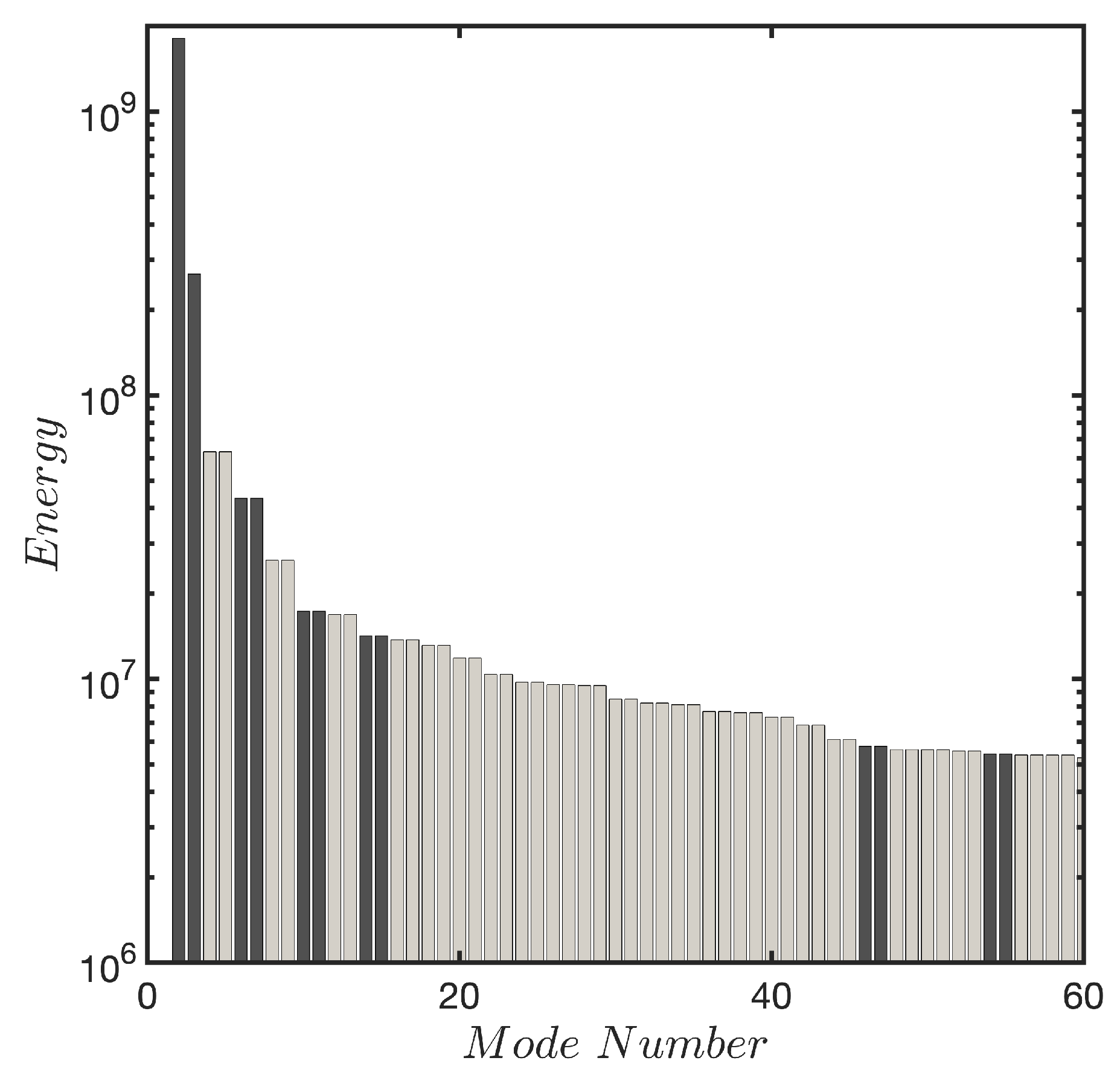
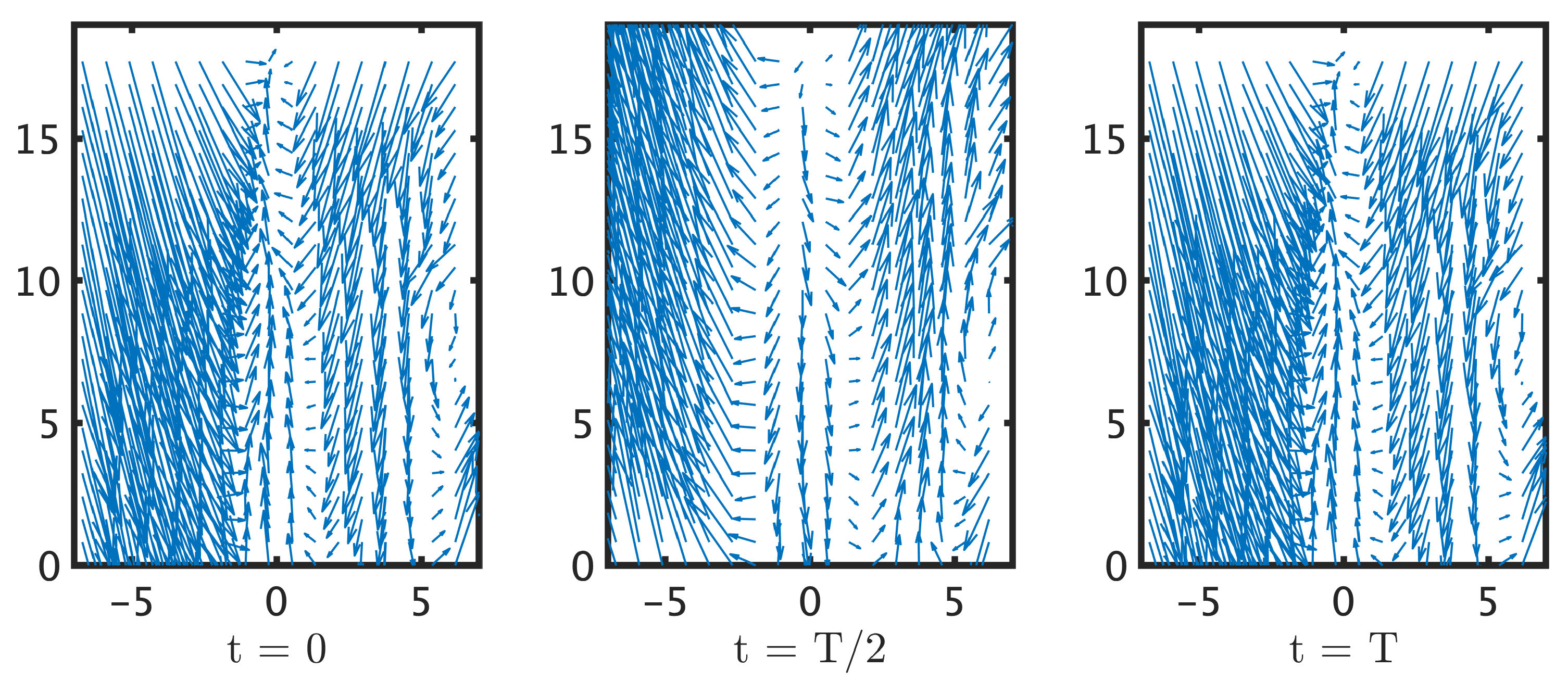
Implementing RMA with and gives 12 robust modes in addition to the mean flow, which together contain approximately 16% of the energy. Figure 10 shows the energy in the first 60 modes, illustrating that robust modes are not those with the highest energy. In particular, this observation implies that POD [15,16,17,18,19] or other energy-based modal decompositions cannot be used to identify robust modes. Flow patterns associated with one of the robust modes whose period is ms is shown in Figure 11.
The origin of the robust cyclic modes in a given configuration is difficult to gauge. They may originate from the flow dynamics, details of the experimental setup, such as imperfections in the inlet flow, or from extraneous factors, such as acoustic reflections from laboratory walls. Our goal is to test whether they need to be eliminated from the turbulent flow prior to computing statistical objects.
5.3. Velocity Fluctuations and Structure Functions
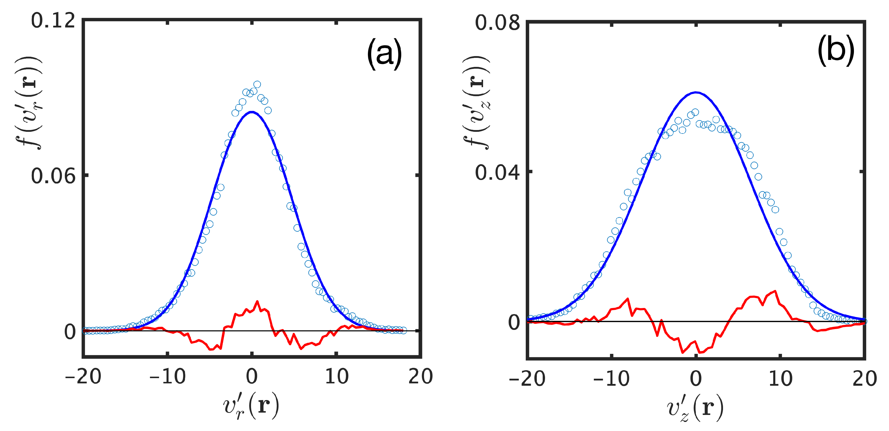
Theoretical studies on statistical properties of turbulent flows, derived on the basis of general considerations such as energy transmission between scales, rely on the isotropy and homogeneity of the flow [6,46,47,48]. Unfortunately, turbulent jet flows are inhomogeneous and do not satisfy these scaling laws [45]. We derive a possible comparison that relies on the empirical observation, illustrated in Figure 12, that point-wise velocity fluctuations in the jet flow, both in axial and radial directions, are approximately Gaussian distributed. We focus on axial velocity fluctuations, , which are distributed as
Although standard deviations are location-dependent, the near-normality of point-wise fluctuations is found at all sites.
The next step is to evaluate the joint distribution of and of axial velocity fluctuations at points and . Although these velocity fluctuations are expected to be uncorrelated at large distances, this fails to hold for the short duration (∼6 ms) of the experiment. However, the variance-covariance matrix for fluctuations between and can be evaluated from the flow data. The joint distribution of and is found to be nearly a centered bivariate normal distribution
whose form is evaluated from the time-series and .
Our goal is to compute structure functions [7,8,46] of all orders using the distribution of the velocity difference . The first step toward this goal is the diagonalization of the variance-covariance matrix. Denote the eigenvalues and eigenvectors of by and . The new variables are distributed on uncorrelated normal distributions with variances and . Next, let the angle between the original basis and the (orthonormal) basis be . The projections of a point to the new eigen-basis are . It can then shown that the difference
with and .
Correlations between velocity fluctuations at neighboring sites are characterized using the family of structure functions
where is the unit vector in the direction . Increasing emphasizes larger deviations from the mean. Structure functions are homogeneous on the symmetry axis, that is, they do not depend on the “origin” [45], as confirmed empirically. Our computations of structure functions are implemented on a 60 ms (6000-frame) segment of the flow. Using Equation (10), it is found that
Any deviation from this expression is due to the slight differences from normality of velocity fluctuations, see Figure 12.
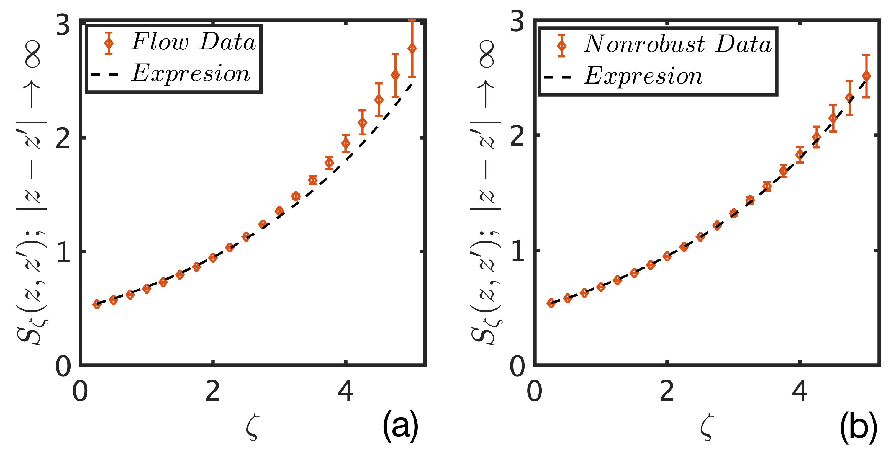
Figure 13a shows structure functions for two points separated by 10.7 mm (40 lattice points) along the symmetry axis. The computation is implemented for four such sets and . (For these points , , and .) The diamonds in Figure 13a are the averages and the error bars are the associated standard deviations of . The data differ from the expression (12), shown by the dashed line.
The corresponding comparison for non-robust constituents of the jet flow is shown in Figure 13b. Now we find excellent agreement. (The dashed line here is computed from the non-robust flow.) This subtle test suggests the need to eliminate robust flow constituents prior to testing statistical theories of turbulent flows.
6. Discussion and Conclusions
We introduced a model-free methodology to extract, from experimental data, the primary constituents in a flow. The methodology is expected to be particularly useful in studying strongly driven fluid or combustion flows [1,2,5,6,7,8], where nonlinearities of the underlying flow induce chaotic dynamics [9]. The lack of precise governing equations, absence of symmetries or other simplifying constraints in realistic configurations, and the presence of flow structures over a wide range of scales reinforce the importance of direct analysis of experimental data.
The proposed approach was predicated on the assumption that primary constituents in fluid or combustion flows are common in multiple, nominally identical realizations of an experiment [31,32,33]. Further, it is assumed that these flow constituents are combinations of dynamic modes that are common between the different experimental realizations, the commonality established via proximity of the eigenvalues and eigenfunctions. Flow constituents are constructed by summing over robust dynamic modes with the same phase dynamics. It needs to be emphasized that, while evaluations of dynamic modes are often fickle, depending sensitively on the precise collection of frames and sites selected for the analysis [29,34,35], robust modes do not suffer this fate.
Robust cyclic facets of a flow may consist of measurement errors, and factors (acoustic reflections from laboratory walls, etc.) extraneous to the system studied. In addition, small-scale features like eddies may be assigned a non-robust designation as well when their appearance, location, and dynamics depend on chaotic aspects of the global flow, that is, they are not cyclical.
We illustrated the use of robust mode analysis (RMA) in a lean combustion flow behind a v-shaped symmetric bluff body, where vortex shedding takes both symmetric and von Karman forms. RMA yielded five robust modes from which two flow constituents were constructed using their phase velocities. One constituent appears to describe symmetric vortex shedding, and the other von Karman shedding. RMA analysis in rich mixtures only yield the first constituent [31]. The approach outlined here was shown to be capable of extracting known flow constituents in shear coaxial jets with and without transverse acoustic driving [32] and in stable and unstable turbulent swirling reacting flows [33].
Difficulties in extracting spatio-temporal flow fields in working engines and reactors motivate us to inquire if RMA can be implemented using time-series from a limited number of point sources such as pressure transducers or temperature sensors, which are implanted in many such systems. We used time-series from nine transducers to study, once again, reacting flows behind a bluff body in lean and rich mixtures. The analysis required synthetically extending the data space [24,27,39,49], in our case, using Chebyshev polynomials. Once again, RMA yielded a single robust mode in rich mixtures and two in lean mixtures. Moreover, the values of one of the robust modes was (nearly) identical at symmetrically-placed transducers, suggesting that the mode represents symmetric vortex shedding.
The final issue we addressed pertains to turbulent flows, whose characterization requires statical objects [5,6,7,8]. We analyzed velocity field data in an axisymmetric turbulent jet flow of Reynolds number ≈21,000, which was shown to contain 13 robust modes. The question we raised is whether statistical characterizations apply to the full flow field or only to its non-robust constituents. We proposed a test that relied on an empirical observation that joint velocity fluctuations were distributed on centered bivariate normal distributions, from which the behavior of structure functions of all orders can be derived. The expression shows closer agreement with non-robust flow fields than with the full flow, suggesting that statistical comparisons of turbulent flows may be better tested on non-robust flow constituents.
The ability to extract robust flow constituents directly from experimental data and to identify their metamorphoses can have broad ranging applications, especially as a signature of impending catastrophic failure in working engines or industrial reactors. It would prove especially useful if the analysis can be implemented using data from easily embedded pressure transducers or thermocouples. Further studies are needed to test if observable changes in flow structures due to progressive material degradation/wear-and-tear precede catastrophic failure of a system.
Author Contributions
Investigation, G.H.G. and S.R. All authors have read and agreed to the published version of the manuscript.
Funding
This research received no external funding.
Institutional Review Board Statement
Not applicable.
Informed Consent Statement
Not applicable.
Data Availability Statement
The spatio-temporal flow velocity data that support the findings of this study, in Matlab format, have been deposited in “figshare.com”, with the accession code “10.6084/m9.figshare. 12789926.” Grid points x and y of the lattice and the velocity fields and in the x and y directions are given for jet flows at Reynolds number 21000.
Acknowledgments
It is a pleasure to thank our collaborators Andrew Caswell, Jia-Chen Hua, Chris Fugger, Terrence Meyer, Joseph Miller, ad Anup Saha who made invaluable contributions to the work discussed here. This manuscript is cleared for public release by the Air Force Research Laboratory (AFRL-2021-0983).
Conflicts of Interest
The authors declare no conflict of interest.
References
- Lieuwen, T. Unsteady Combustor Physics; Cambridge University Press: Cambridge, UK, 2012. [Google Scholar]
- Joulin, G.; Sivashinsky, G. On the Dynamics of Nearly-Extinguished Non-Adiabatic Cellular Flames. Combust. Sci. Technol. 1983, 31, 75–90. [Google Scholar] [CrossRef]
- Kostka, S.; Lynch, A.C.; Huelskamp, B.C.; Kiel, B.V.; Gord, J.R.; Roy, S. Characterization of Flame-Shedding Behavior Behind a Bluff-Body Using Proper Orthogonal Decomposition. Combust. Flame 2012, 159, 2872–2882. [Google Scholar] [CrossRef]
- Viswanathan, G.; Sheintuch, M.; Luss, D. Transversal hot zones formation in catalytic packed-bed reactors. Ind. Eng. Chem. Res. 2008, 47, 2509–2523. [Google Scholar] [CrossRef]
- Chandrasekhar, S. Hydrodynamic and Hydromagnetic Stability; Dover Publications, Inc.: New York, NY, USA, 1961. [Google Scholar]
- Frisch, U. Turbulence: The Legacy of A. N. Kolmogorov; Cambridge University Press: Cambridge, UK, 1995. [Google Scholar]
- Monin, A.S.; Yaglom, A.M. Statistical Fluid Mechanics, Mechanics of Turbulence; Dover Publications, Inc.: New York, NY, USA, 1971; Volume I. [Google Scholar]
- Monin, A.S.; Yaglom, A.M. Statistical Fluid Mechanics, Mechanics of Turbulence; Dover Publications, Inc.: New York, NY, USA, 1971; Volume II. [Google Scholar]
- Cross, M.C.; Hohenberg, P.C. Pattern formation outside of equilibrium. Rev. Mod. Phys. 1993, 65, 851. [Google Scholar] [CrossRef] [Green Version]
- Raffel, M.; Willert, C.; Wereley, S.; Kompenhans, J. Particle Image Velocimetry: A Practical Guide; Springer: Cham, Switzerland, 2007. [Google Scholar]
- Westerweek, A. Particle Image Velocimetry; Cambridge University Press: Cambridge, UK, 2011. [Google Scholar]
- Seitzman, J.M.; Hanson, R.K. Planar Fluorescence Imaging in Gases. In Instrumentation for Flows with Combustion; Taylor, A.M.K.P., Ed.; Academic Press: London, UK, 1993. [Google Scholar]
- Steinfeld, J.I.; Francisco, J.S.; Hase, W.L. Chemical Kinetics and Dynamics; Prentice-Hall: Hoboken, NJ, USA, 1998. [Google Scholar]
- Faltinsen, O.M.; Timokha, A.N. Sloshing; Cambridge University Press: Cambridge, UK, 2009. [Google Scholar]
- Lumley, J.L. The Structure of Inhomogeneous Flow. In Atmospheric Turbulence and Radio Wave Propagation; Publishing House Nauka: Moscow, Russia, 1967; pp. 166–176. [Google Scholar]
- Berkooz, G.; Holmes, P.; Lumley, J.L. The Proper Orthogonal Decomposition in the Analysis of Turbulent Flows. Annu. Rev. Fluid Mech. 1993, 25, 539–575. [Google Scholar] [CrossRef]
- Sirovich, L. Turbulence and the Dynamics of Coherent Structures. 1. Coherent Structures. Q. Appl. Math. 1987, 45, 561–571. [Google Scholar] [CrossRef] [Green Version]
- Sirovich, L. Turbulence and the Dynamics of Coherent Structures. 2. Symmetries and Transformations. Q. Appl. Math. 1987, 45, 573–582. [Google Scholar] [CrossRef] [Green Version]
- Sirovich, L. Turbulence and the Dynamics of Coherent Structures. 3. Dynamics and Scaling. Q. Appl. Math. 1987, 45, 583–590. [Google Scholar] [CrossRef] [Green Version]
- Schmid, P.J. Dynamic mode decomposition of experimental data. In Proceedings of the 8th International Symposium on Particle Image Velocimetry, PIV09-0141, Melbourne, VIC, Australia, 25–28 August 2009. [Google Scholar]
- Schmid, P.J. Dynamic Mode Decomposition of Numerical and Experimental Data. J. Fluid Mech. 2010, 656, 5–28. [Google Scholar] [CrossRef] [Green Version]
- Rowley, C.W.; Mezic, I.; Bagheri, S.; Schlatter, P.; Henningson, D.S. Spectral Analysis of Nonlinear Flows. J. Fluid Mech. 2009, 641, 115–127. [Google Scholar] [CrossRef] [Green Version]
- Mezic, I. Analysis of Fluid Flows via Spectral Properties of the Koopman Operator. Annu. Rev. Fluid Mech. 2013, 45, 357–378. [Google Scholar] [CrossRef] [Green Version]
- Kutz, J.N.; Brunton, S.L.; Brunton, B.W.; Proctor, J.L. Dynamic Mode Decomposition: Data-Driven Modeling of Complex Systems; Society for Industrial and Applied Mathematics: Philadelphia, PA, USA, 2016. [Google Scholar]
- Budiši´c, M.; Mohr, R.M.; Mezi´c, I. Applied Koopmanism. Chaos 2012, 22, 047510. [Google Scholar] [CrossRef] [Green Version]
- Chen, K.K.; Tu, J.H.; Rowley, C.W. Variants of dynamic mode decomposition: Boundary condition, Koopman and Fourier analysis. J. Nonlinear Sci. 2012, 22, 887–915. [Google Scholar] [CrossRef]
- Williams, M.O.; Rowley, C.W.; Kevrikidis, I.G. A kernal-based approach to data-driven Koopman spectral analysis. arXiv 2016, arXiv:1411.2260. [Google Scholar]
- Bouwmans, T.; Sobral, A.; Javed, S.; Jung, S.K.; Zahzah, E.-H. Decomposition into low-rank plus additive matrices for background/foreground separation: A review for a comparative eveluation with a large-scale dataset. Comput. Sci. Rev. 2017, 23, 1–71. [Google Scholar] [CrossRef] [Green Version]
- Scherl, I.; Strom, B.; Shang, J.K.; Williams, O.; Polagye, B.L.; Brunton, S.L. Robust principal components analysis for modal decomposition of corrupt fluid flows. Phys. Rev. Fluids 2020, 5, 054401. [Google Scholar] [CrossRef]
- Choi, H.; Jeon, W.-P.; Kim, J. Control of flow over a bluff body. Annu. Rev. Fluid Mech. 2008, 40, 113–139. [Google Scholar] [CrossRef] [Green Version]
- Roy, S.; Hua, J.-C.; Barnhill, W.; Gunaratne, G.H.; Gord, J.R. Deconvolution of reacting-flow dynamics using proper orthogonal and dynamic mode decompositions. Phys. Rev. E 2015, 91, 013001. [Google Scholar] [CrossRef] [Green Version]
- Hua, J.-C.; Gunaratne, G.H.; Talley, D.G.; Gord, J.R.; Roy, S. Dynamic-mode decomposition based analysis of shear coaxial jets with and without transverse acoustic driving. J. Fluid Mech. 2016, 790, 5–32. [Google Scholar] [CrossRef]
- Roy, S.; Yi, T.; Jiang, N.; Gunaratne, G.H.; Chterev, I.; Emerson, B.; Lieuwen, T.; Caswell, A.W.; Gord, J.R. Dynamics of robust structures in turbulent swirling reacting flows. J. Fluid Mech. 2017, 816, 554–585. [Google Scholar] [CrossRef]
- Bagheri, S. Effects of weak noise on oscillating flows: Linking quality factor, Floquet modes, and Koopman spectrum. Phys. Fluids 2014, 26, 094104. [Google Scholar] [CrossRef] [Green Version]
- Dawson, S.T.M.; Hemati, M.S.; Williams, M.O.; Rowley, C.W. Characterizing and correcting for the effect of sensor noise in the dynamic mode decomposition. Exp. Fluids 2016, 57, 42. [Google Scholar] [CrossRef] [Green Version]
- Huang, L.-Z.; Nie, D.-M. Vortex Shedding Patterns in Flow Past Inline Oscillating Elliptical Cylinders. Therm. Sci. 2012, 16, 1395–1399. [Google Scholar] [CrossRef]
- Konstantinidis, E.; Balabani, S. Symmetric vortex. shedding in the near wake of a circular cylinder due to streamwise perturbations. J. Fluids Struct. 2007, 23, 1047–1063. [Google Scholar] [CrossRef]
- Caswell, A.W.; Jiang, N.; Roy, S.; Huelskamp, B.; Monfort, J.; Lynch, A.; Belovich, V.M.; Gord, J.R. High-repetition-rate OH-PLIF and PIV measurements in bluff body stabilized flames. In Proceedings of the 52nd Aerospace Sciences Meeting, Harbor, MD, USA, 13–17 January 2014. [Google Scholar] [CrossRef]
- Li, Q.; Dietrich, F.; Bolt, E.M.; Kevrikidis, I.G. Extended dynamic mode decomposition with dictionary learning: A data-driven adaptive spectral decomposition of the Koopman operator. Chaos 2017, 27, 103111. [Google Scholar] [CrossRef]
- Suresh, S. Fatigue of Materials; Cambridge University Press: Cambridge, UK, 2004. [Google Scholar]
- Kim, W.H.; Laird, C. Crack nucleation and stage i propagation in high strain fatigue—II mechanism. Acta Metall. 1978, 26, 789–799. [Google Scholar] [CrossRef]
- Fugger, C.A.; Roy, S.; Caswell, A.W.; Rankin, B.A.; Gord, J.R. Structure and dynamics of CH2O, OH, and the velocity field of a confined bluff-body premixed flame, using simultaneous PLIF and PIV at 10 kHz. Proc. Combust. Inst. 2019, 37, 1461–1469. [Google Scholar] [CrossRef]
- Slipchenko, M.; Miller, J.D.; Roy, S.; Meyer, T.R.; Mance, J.G.; Gord, J.R. 100-kHz, 100-ms, 400-J Burst-Mode Laser with Dual-Wavelength Diode-Pumped Amplifiers. Opt. Lett. 2014, 39, 4735–4738. [Google Scholar] [CrossRef] [PubMed] [Green Version]
- Miller, J.D.; Jiang, N.; Slipchenko, M.N.; Mance, J.; Gmeyer, T.R.; Roy, S.; Gord, J.R. Spatiotemporal analysis of turbulent jets enabled by 100-kHz, 100-ms burst-mode particle image velocimetry. Exp. Fluids 2016, 57, 192. [Google Scholar] [CrossRef]
- Roy, S.; Miller, J.; Gunaratne, G.H. Deviations from Taylor’s Frozen Hypothesis and Scaling Laws in Inhomogeneous Jet Flows. Commun. Phys. 2021, 4, 32. [Google Scholar] [CrossRef]
- Kolmogorov, A.N. Local structure of turbulence in an incompressible fluid at very high Reynolds numbers. Dokl. Akad. Naud. SSSR 1941, 30, 299–303. [Google Scholar] [CrossRef]
- Kolmogorov, A.N. Energy dissipation in locally isotropic turbulence. Dokl. Akad. Naud. SSSR 1941, 32, 19–21. [Google Scholar]
- Obukhov, A.M. Energy distribution in the spectrum of a turbulent flow. Izvestiya Akad. Nauk. SSSR Ser. Geogr. Geofiz. 1941, 4–5, 453–466. [Google Scholar]
- Williams, M.O.; Kevrikidis, I.G.; Rowley, C.W. A data-driven approximation of the Koopman operator: Extending dynamic mode decomposition. J. Nonlinear Sci. 2016, 25, 1307–1346. [Google Scholar] [CrossRef] [Green Version]
Figure 1.
The number of robust modes found in the turbulent jet flow analyzed in Section 5 as a function of when the cutoff is set at 0.75.
Figure 1.
The number of robust modes found in the turbulent jet flow analyzed in Section 5 as a function of when the cutoff is set at 0.75.

Figure 2.
(a) Schematic of the reacting flow behind a v-gutter bluff body (adapted from the Ref. [38]). Schematics showing (b) symmetric and (c) von Karman vortex shedding behind a symmetric barrier.
Figure 2.
(a) Schematic of the reacting flow behind a v-gutter bluff body (adapted from the Ref. [38]). Schematics showing (b) symmetric and (c) von Karman vortex shedding behind a symmetric barrier.

Figure 3.
(a) The DMD spectrum for the reacting flow for a “lean” mixture with equivalence ratio (adapted from the Ref. [31]). The flow exhibits symmetric vortex shedding, as well as von Karman shedding at this equivalence ratio. (b) The mean and standard deviation for the robust modes 4, 5, 38, 58, and 61.

Figure 4.
(a) Real and (b) imaginary parts of , the symmetric mode with the largest energy, for the reacting flow at . (c) Real and (d) imaginary parts of , the asymmetric mode with the highest energy. This figure was adapted from the Ref. [31].
Figure 4.
(a) Real and (b) imaginary parts of , the symmetric mode with the largest energy, for the reacting flow at . (c) Real and (d) imaginary parts of , the asymmetric mode with the highest energy. This figure was adapted from the Ref. [31].

Figure 5.
Phase dynamics of robust modes for the reacting flow. “Angular velocities” radians/frame and radians/frame are nearly identical, suggesting that they belong to the same flow constituent. ( is slightly higher and is not used in the reconstruction.) Similarly, radian/frame and radians/frame are close, suggesting that they form a second constituent. Successive curves are shifted for clarity. This figure was adapted from the Ref. [31].

Figure 6.
Several snapshots of the reacting flow at equivalence ratio (top row), reconstructions of the symmetric (second row), and asymmetric (bottom row) flow constituents. This figure was adapted from the Ref. [31].
Figure 6.
Several snapshots of the reacting flow at equivalence ratio (top row), reconstructions of the symmetric (second row), and asymmetric (bottom row) flow constituents. This figure was adapted from the Ref. [31].

Figure 7.
Schematic of the bluff body combustion chamber with locations of pressure transducers. The trailing edge of the symmetric bluff body is assigned to be at downstream locations being positive. Note that transducers 7, 8, and 9 are placed opposite to 4, 5, and 6, respectively. A detailed explanation of imaging optics and measurement techniques can be found in the Ref. [42]. Here, we confine our analysis to measurements from transducers 1–9.

Figure 8.
(a) Symmetric robust mode: Projections of the single robust mode at . The x-axis is the transducer number, and the y-axis the magnitude of the robust mode at the site. Note that values of the mode on sites 4, 5, and 6 are nearly identical to those at sites 7, 8, and 9. Pairs of transducers (4, 7), (5, 8), and (6, 9) are at identical axis locations, thus indicating that the robust mode represents a symmetric flow constituent. (b) Asymmetric robust mode: One robust modes of the flow at . Note that it does not have the symmetry between the values at transducer pairs (4, 7), (5, 8) and (6, 9) seen in the mode of (a).

Figure 9.
(a) Axisymmetric jet flow is generated by gas ejected from cylinder of radius mm. Rectangular region of size mm × mm where velocity measurements were made is approximately downstream of inlet. (b) Snapshot of velocity field for flow of 21,000.
Figure 9.
(a) Axisymmetric jet flow is generated by gas ejected from cylinder of radius mm. Rectangular region of size mm × mm where velocity measurements were made is approximately downstream of inlet. (b) Snapshot of velocity field for flow of 21,000.

Figure 10.
The energy of the first 60 dynamic modes. Robust modes are shown in the dark color. Note that robust modes are not those with the highest energy.
Figure 10.
The energy of the first 60 dynamic modes. Robust modes are shown in the dark color. Note that robust modes are not those with the highest energy.

Figure 11.
Flow patterns in the pair of robust modes 6 and 7 whose eigenvalues are and whose period is ms.
Figure 11.
Flow patterns in the pair of robust modes 6 and 7 whose eigenvalues are and whose period is ms.

Figure 12.
Distributions of (a) radial, and (b) axial velocity fluctuations at a fixed location. The blue lines are the best Gaussian fit to the data and red lines are deviations from the Gaussian.
Figure 12.
Distributions of (a) radial, and (b) axial velocity fluctuations at a fixed location. The blue lines are the best Gaussian fit to the data and red lines are deviations from the Gaussian.

Figure 13.
(a) The diamonds show as a function of the moment for for the jet flow. The dashed line is that given in Equation (12). (b) The corresponding comparison for the non-robust flow.
Figure 13.
(a) The diamonds show as a function of the moment for for the jet flow. The dashed line is that given in Equation (12). (b) The corresponding comparison for the non-robust flow.

Publisher’s Note: MDPI stays neutral with regard to jurisdictional claims in published maps and institutional affiliations. |
© 2021 by the authors. Licensee MDPI, Basel, Switzerland. This article is an open access article distributed under the terms and conditions of the Creative Commons Attribution (CC BY) license (https://creativecommons.org/licenses/by/4.0/).
Share and Cite
MDPI and ACS Style
Gunaratne, G.H.; Roy, S. Robust Mode Analysis. Mathematics 2021, 9, 1057. https://doi.org/10.3390/math9091057
AMA Style
Gunaratne GH, Roy S. Robust Mode Analysis. Mathematics. 2021; 9(9):1057. https://doi.org/10.3390/math9091057
Chicago/Turabian StyleGunaratne, Gemunu H., and Sukesh Roy. 2021. "Robust Mode Analysis" Mathematics 9, no. 9: 1057. https://doi.org/10.3390/math9091057
Note that from the first issue of 2016, this journal uses article numbers instead of page numbers. See further details here.