
Learning Neural Representations and Local Embedding for Nonlinear Dimensionality Reduction Mapping


Abstract
:1. Introduction
2. Materials and Methods
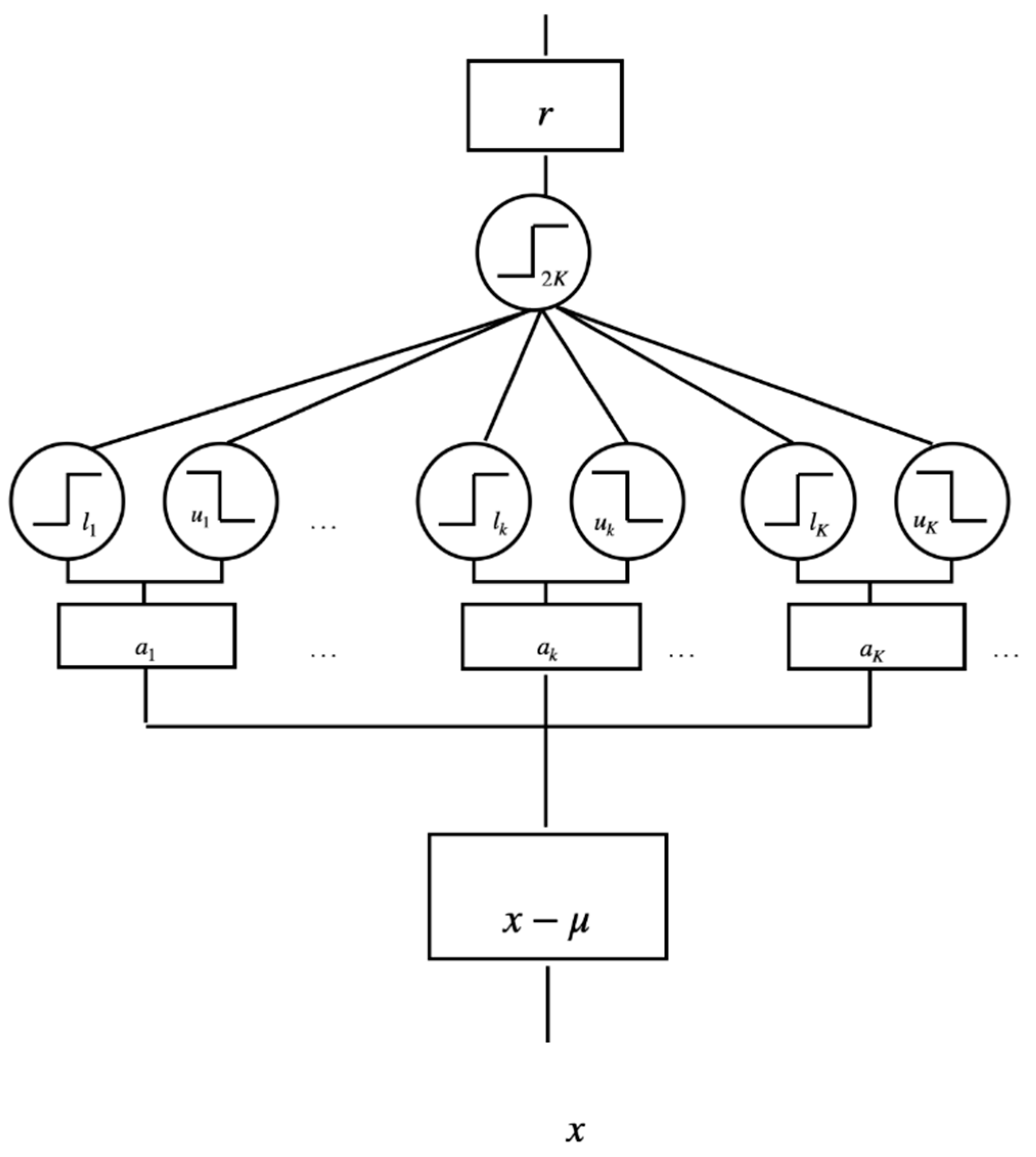
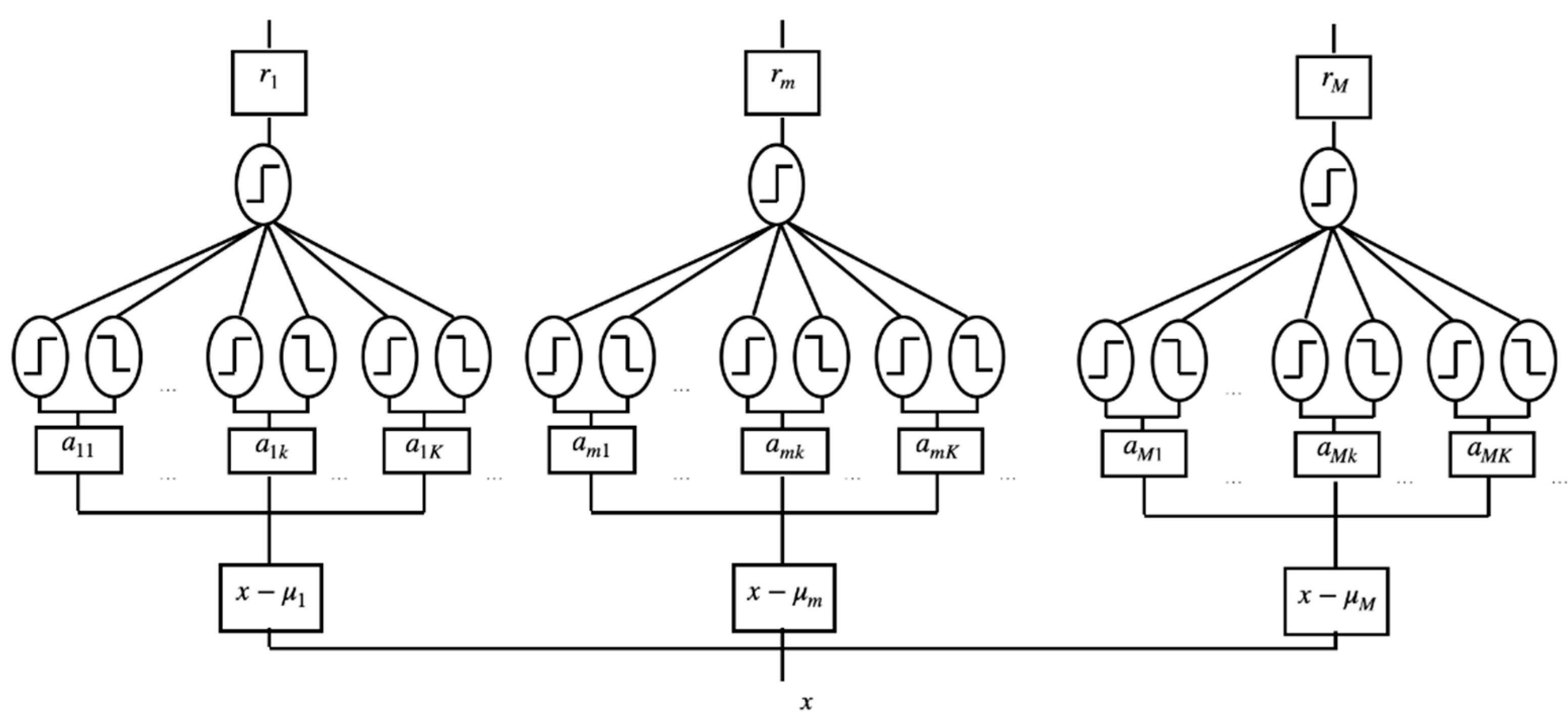
2.1. Adaline Neural Modules for Representing Distributed Data Supports
2.2. NDR Model Learning
2.2.1. Clustering Analysis for Learning Receptive Fields
2.2.2. Deriving Cluster Supports by Optimizing Adaline Modules
2.2.3. Graph Configuration and Neighboring Relations of Cluster Supports
2.3. Levenberg-Marquardt Learning for Distance-Preserving Mapping and Optimal Posterior Weights
2.4. Locally Nonlinear Embedding for NDR Mapping
3. Results
4. Discussion
5. Conclusions
Author Contributions
Funding
Informed Consent Statement
Data Availability Statement
Conflicts of Interest
Appendix A
- Randomly set all near the mean of all data points, , initialize the inverse temperature parameter β to sufficiently low value, and set to a small positive value.
- Calculate the distance between each point and .
- Update the expectation of each element in exclusive memberships. .
- Set stability to the mean of over . If stability is less than the sum of and , add each with a small andom noise for perturbation.
- Fix all and minimize the with respect to all .
- If stability < 0.98, set β to β/0.995 and repeat Step ii-v, otherwise halt.
References
- Roweis, S.; Saul, L. Nonlinear dimensionality reduction by locally linear embedding. Science 2000, 290, 2323–2326. [Google Scholar] [CrossRef] [PubMed] [Green Version]
- Tenenbaum, J.; Silva, d.V.; Langford, J. A global geometric framework for nonlinear dimensionality reduction. Science 2000, 290, 2319–2323. [Google Scholar] [CrossRef] [PubMed]
- Hinton, G.; Salakhutdinov, R. Reducing the dimensionality of data with neural networks. Science 2006, 313, 504–507. [Google Scholar] [CrossRef] [Green Version]
- Sorzano, C.O.S.; Vargas, J.; Pascual-Montano, A.D. A Survey of Dimensionality Reduction Techniques. arXiv 2014, arXiv:1403.2877. [Google Scholar]
- Afshar, M.; Usefi, H. High-dimensional feature selection for genomic datasets. Knowl. Based Syst. 2020, 206, 106370. [Google Scholar] [CrossRef]
- Rabin, N.; Kahlon, M.; Malayev, S. Classification of human hand movements based on EMG signals using nonlinear dimen-sionality reduction and data fusion techniques. Expert Syst. Appl. 2020, 149, 113281. [Google Scholar] [CrossRef]
- Taskin, G.; Crawford, M.M. An Out-of-Sample Extension to Manifold Learning via Meta-Modelling. IEEE Trans. Image Process. 2019, 28, 5227–5237. [Google Scholar] [CrossRef] [PubMed]
- Li, H. 1D representation of Laplacian eigenmaps and dual k-nearest neighbours for unified video coding. IET Image Process. 2020, 14, 2156–2165. [Google Scholar] [CrossRef]
- Pearson, K.F.R.S. LIII. On lines and planes of closest fit to systems of points in space. Lond. Edinb. Dublin Philos. Mag. J. Sci. 1901, 2, 559–572. [Google Scholar] [CrossRef] [Green Version]
- Hotelling, H. Analysis of a complex of statistical variables into principal components. J. Edu. Psychol. 1933, 24, 417–441. [Google Scholar] [CrossRef]
- Belkin, M.; Niyogi, P. Laplacian eigenmaps and spectral techniques for embedding and clustering. In Advances in Neural Information Processing Systems (NIPS 2001); Dietterich, T., Becker, S., Ghahramani, Z., Eds.; MIT Press: Cambridge, MA, USA, 2002. [Google Scholar]
- Donoho, D.; Grimes, C. Hessian eigenmaps: Locally linear em-bedding techniques for high-dimensional data. Proc. Natl. Acad. Sci. USA 2003, 100, 5591–5596. [Google Scholar] [CrossRef] [Green Version]
- Torgerson, W.S. Multidimensional scaling: I. Theory and method. Psychometrika 1952, 17, 401–419. [Google Scholar] [CrossRef]
- Young, G.; Householder, A.S. Discussion of a set of points in terms of their mutual distances. Psychometrika 1938, 3, 19–22. [Google Scholar] [CrossRef]
- Sammon, J. A nonlinear mapping algorithm for data structure analysis. IEEE Trans. Comput. 1969, 100, 401–409. [Google Scholar] [CrossRef]
- Kohonen, T. Self-organized formation of topologically correct feature maps. Biol. Cybern. 1982, 43, 59–69. [Google Scholar] [CrossRef]
- Ritter, H.; Martinetz, T.; Schulten, K. Reading. Neural Computation and Self-Organizing Maps; Addison-Wesley: Boston, MA, USA, 1992. [Google Scholar]
- Kohonen, T. Self-Organizing Maps, 2nd ed.; Springer: Berlin/Heidelberg, Germany, 1995. [Google Scholar]
- Hu, R.; Ratner, K.; Ratner, E. ELM-SOM plus: A continuous mapping for visualization. Neurocomputing 2019, 365, 147–156. [Google Scholar] [CrossRef]
- Durbin, R.; Willshaw, G. An analogue approach to the traveling salesman problem using an elastic net method. Nature 1987, 326, 689–691. [Google Scholar] [CrossRef] [PubMed]
- Durbin, R.; Mitchison, G. A dimension reduction framework for cortical maps. Nature 1990, 343, 644–647. [Google Scholar] [CrossRef]
- Widrow, B.; Lehr, M. 30 years of adaptive neural networks: Perceptron, Madaline, and backpropagation. Proc. IEEE 1990, 78, 1415–1442. [Google Scholar] [CrossRef]
- Wu, J.-M.; Lin, Z.-H.; Hsu, P.-H. Function approximation using generalized adalines. IEEE Trans. Neural Netw. 2006, 17, 541–558. [Google Scholar] [CrossRef]
- Hagan, M.; Menhaj, M. Training feedforward networks with the Marquardt algorithm. IEEE Trans. Neural Netw. 1994, 5, 989–993. [Google Scholar] [CrossRef]
- Ljung, L. System Identification—Theory for the User; Prentice-Hall: Hoboken, NJ, USA; Englewood Cliffs: Bergen, NJ, USA, 1987. [Google Scholar]
- NØrgaard, M.; Ravn, O.; Poulsen, N.K.; Hansen, L.K. Neural Networks for Modelling and Control of Dynamic Systems; Springer: Berlin/Heidelberg, Germany, 2000. [Google Scholar]
- Wu, J.-M. Multilayer Potts Perceptrons with Levenberg–Marquardt Learning. IEEE Trans. Neural Netw. 2008, 19, 2032–2043. [Google Scholar] [CrossRef] [PubMed]
- Wu, J.-M.; Hsu, P.-H. Annealed Kullback—Leibler divergence minimization for generalized TSP, spot identification and gene sorting. Neurocomputing 2011, 74, 2228–2240. [Google Scholar] [CrossRef]
- Wu, J.-M.; Lin, Z.-H. Learning generative models of natural images. Neural Netw. 2002, 15, 337–347. [Google Scholar] [CrossRef]
- Tasoulis, S.; Pavlidis, N.G.; Roos, T. Nonlinear Dimensionality Reduction for Clustering. Pattern Recognit. 2020, 107, 107508. [Google Scholar] [CrossRef]
- Dijkstra, E.W. A note on two problems in connexion with graphs. Numer. Math. 1959, 1, 269–271. [Google Scholar] [CrossRef] [Green Version]
- Hopfield, J.J. Neural networks and physical systems with emergent collective computational abilities. Proc. Natl. Acad. Sci. USA 1982, 79, 2554–2558. [Google Scholar] [CrossRef] [Green Version]
- Hopfield, J.J.; Tank, D.W. “Neural” computation of decisions in optimization problems. Biol. Cybern. 1985, 52, 141–152. [Google Scholar]
- Peterson, C.; Söderberg, B. A New Method for Mapping Optimization Problems onto Neural Networks. Int. J. Neural Syst. 1989, 1, 3–22. [Google Scholar] [CrossRef] [Green Version]
- Wu, J.-M. Potts models with two sets of interactive dynamics. Neurocomputing 2000, 34, 55–77. [Google Scholar] [CrossRef]
- Martin, B.; Jens, L.; André, S.; Thomas, Z. Robust dimensionality reduction for data visualization with deep neural networks. Graph. Models 2020, 108, 101060. [Google Scholar]
- Ding, J.; Condon, A.; Shah, S.P. Interpretable dimensionality reduction of single cell transcriptome data with deep generative models. Nat. Commun. 2018, 9, 1–13. [Google Scholar] [CrossRef] [PubMed] [Green Version]
- LeCun, Y.; Bengio, Y.; Hinton, G. Deep learning. Nature 2015, 521, 436–444. [Google Scholar] [CrossRef] [PubMed]
- Available online: https://lvdmaaten.github.io/drtoolbox/ (accessed on 29 April 2020).


| Reservation Ratio (Testing) | Error Percentage (Testing) | |||
|---|---|---|---|---|
| Dataset | Mean | Var | Mean | Var |
| Brokenswiss | 89.78% | 1.73 × 10⁻⁵ | 3.92% | 6.03 × 10⁻⁵ |
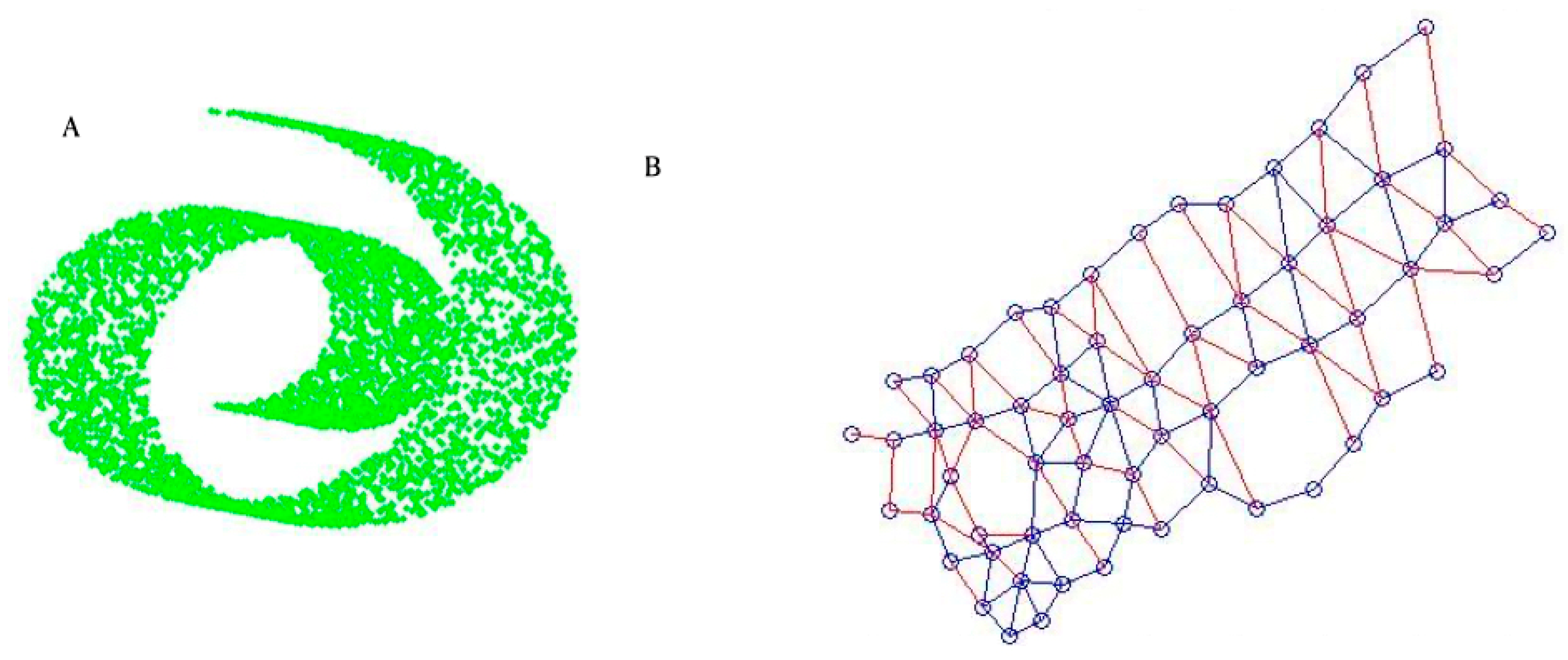
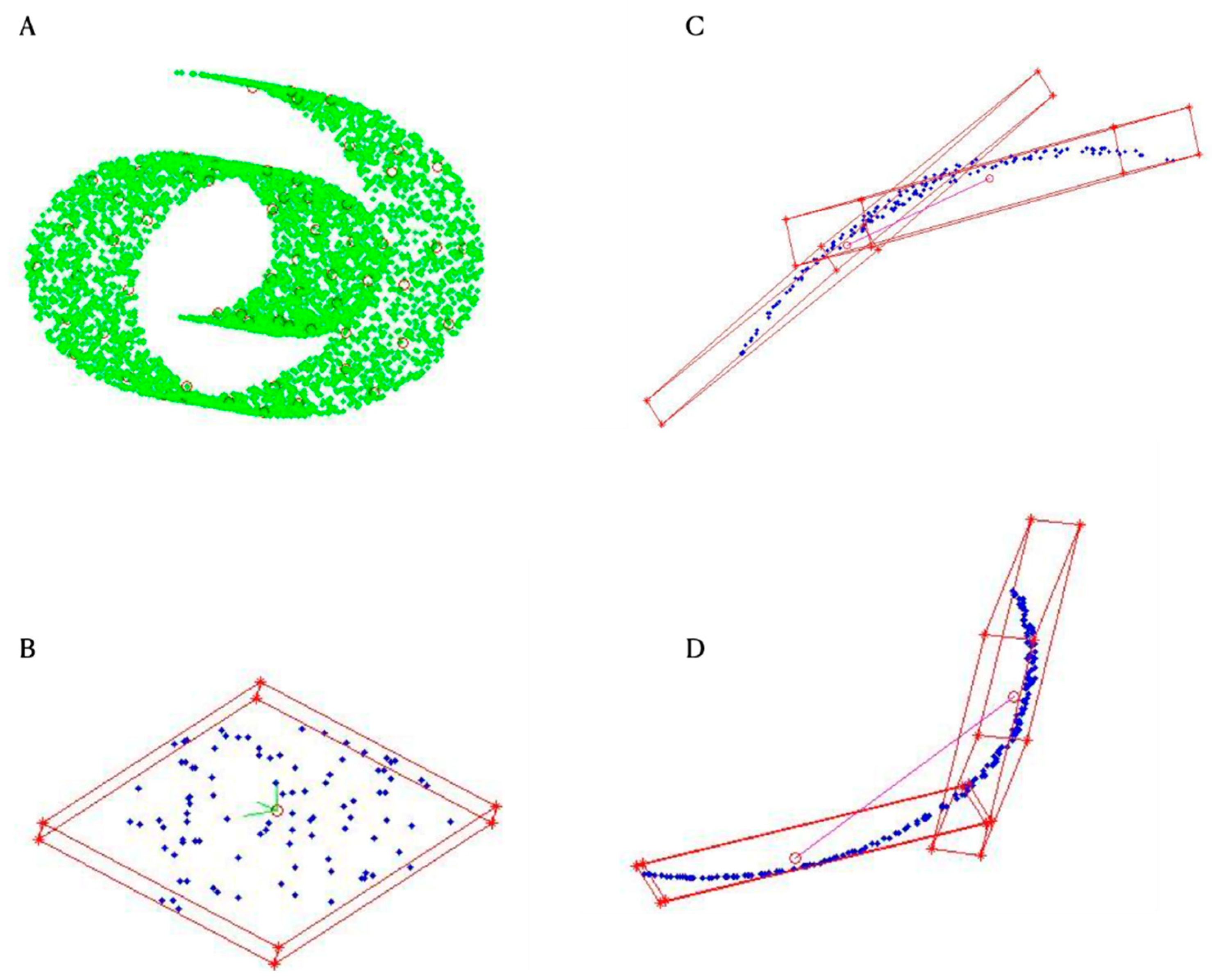
| Colorball | 95.00% | 5.35 × 10⁻⁶ | 16.51% | 2.83 × 10⁻⁵ |
| Execution Time | ||||
|---|---|---|---|---|
| Training (Seconds) | Testing (Seconds) | |||
| Dataset | Mean | Var | Mean | Var |
| Colorball | 166.0 | 66.0 | 190.0 | 43.7 |
Publisher’s Note: MDPI stays neutral with regard to jurisdictional claims in published maps and institutional affiliations. |
© 2021 by the authors. Licensee MDPI, Basel, Switzerland. This article is an open access article distributed under the terms and conditions of the Creative Commons Attribution (CC BY) license (https://creativecommons.org/licenses/by/4.0/).
Share and Cite
Wu, S.-S.; Jong, S.-J.; Hu, K.; Wu, J.-M. Learning Neural Representations and Local Embedding for Nonlinear Dimensionality Reduction Mapping. Mathematics 2021, 9, 1017. https://doi.org/10.3390/math9091017
Wu S-S, Jong S-J, Hu K, Wu J-M. Learning Neural Representations and Local Embedding for Nonlinear Dimensionality Reduction Mapping. Mathematics. 2021; 9(9):1017. https://doi.org/10.3390/math9091017
Chicago/Turabian StyleWu, Sheng-Shiung, Sing-Jie Jong, Kai Hu, and Jiann-Ming Wu. 2021. "Learning Neural Representations and Local Embedding for Nonlinear Dimensionality Reduction Mapping" Mathematics 9, no. 9: 1017. https://doi.org/10.3390/math9091017