Modeling and Estimating Volatility of Day-Ahead Electricity Prices

Abstract

We model day-ahead electricity prices of the UK power market using skew generalized error distribution. This distribution allows us to take into account the features of asymmetry, heavy tails, and a peak higher than in normal or Student’s t distributions. The adequacy of the estimated volatility model is verified using various tests and criteria. A correctly specified volatility model can be used for analyzing the impact of reforms or other events. We find that, after the start of the COVID-19 pandemic, price level and volatility increased.

1. Introduction

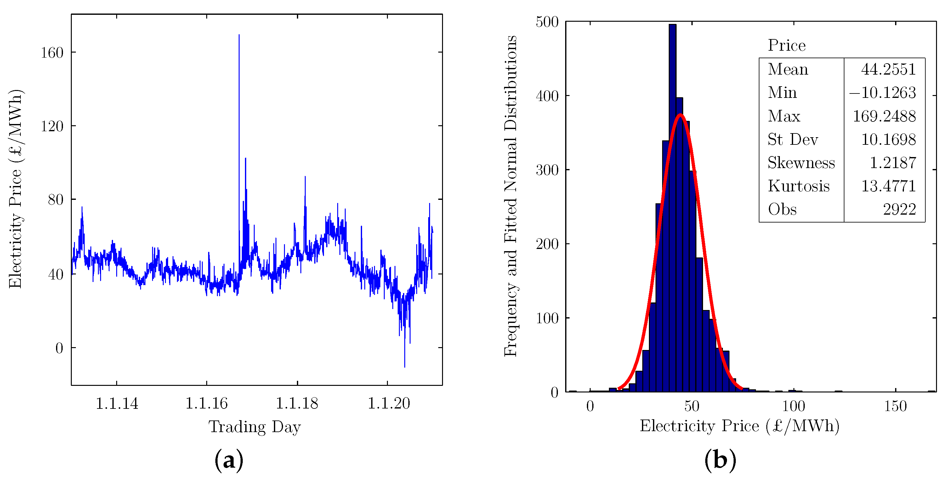
We study electricity prices of the UK power market N2EX. This market is operated as a day-ahead auction and was launched on 12 January 2010 by Nord Pool Spot AS in cooperation with Nasdaq Commodities [1]. The daily price data are summarized in Figure 1. Complete data are available starting from the year 2013. We analyze the price data until 31 December 2020 because we believe that, after the end of the Brexit transition period, the price level and volatility may have changed.

In time series modeling, it is necessary to make a distributional assumption for model residuals. Because the distribution of electricity prices described in Figure 1b is asymmetric and has a peak higher than in the fitted normal distribution, we consider using skew generalized error distribution (SGED). This distribution accommodates features such as asymmetry, heavy tails, and a peak higher than in normal or Student’s t distributions.

Modeling prices can allow us to understand the impact of reforms or other events such as the COVID-19 pandemic. In order to hamper the spread of the COVID-19 pandemic, many countries started to introduce restrictions in March 2020. For example, on 18 March 2020, the UK government announced the closure of schools, which was later followed by the closure of public venues, such as pubs, restaurants, gyms, theatres, etc. The lifestyle, work style, and various sectors of the economy were greatly affected by those restrictions. The global pandemic is still ongoing, and the expected overall effect is generally hard to evaluate.

This paper is structured as follows. First, we review literature on volatility modeling. Then, we describe methodology for modeling volatility of electricity prices. In the next section, the distributional assumptions and the correctness of the estimated volatility model are verified and discussed in detail. Finally, we provide a discussion and draw conclusions related to the methodology of volatility modeling and an analysis of COVID-19 on electricity prices.

2. Literature Review

Reference [2] is the seminal study introducing the autoregressive conditional heteroscedasticity (ARCH) model. The model is applied for estimating the means and variances of inflation in the UK. Later, Reference [3] extended this model to the generalized ARCH (i.e., GARCH). Both of these papers assumed normal distribution for model residuals. Reference [4] introduced the exponential ARCH model, which addresses the shortcomings of the GARCH model. In order to take into account the feature of heavy tails, the author assumed that model residuals follow generalized error distribution (GED), which includes normal distribution as a special case. Reference [4] suggested that replacing normal or Student’s t distributions by generalized error distribution (GED) is more encouraging. This suggestion is based on the fact that GED is heavy tailed compared to normal distribution and does not have an issue of possible infinite unconditional moments, as Student’s t distribution does.

Some research (e.g., [5,6,7,8]) however consider a normal or Student’s t distribution when applying the volatility model of [4] that was based on GED. In order to take into account the feature of heavy tails, Reference [9] assumed that model residuals follow Student’s t distribution, even if the empirical distribution of residuals had a higher peak than in the fitted normal distribution.

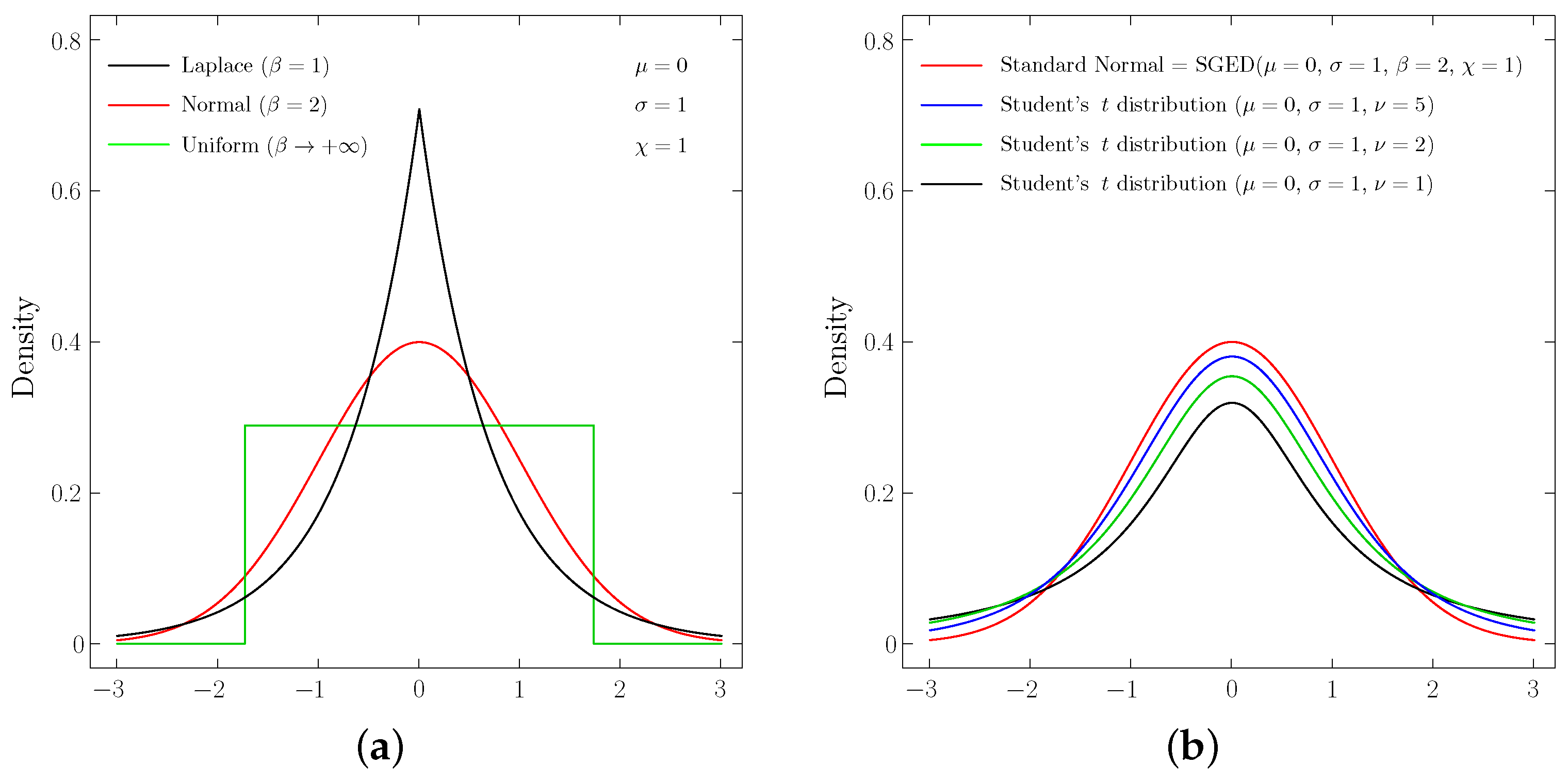
It is well-documented in the literature that heavy tails can be modeled using GED or Student’s t distribution. In Figure 4, we illustrate that the choice between GED and Student’s t distribution should depend on the peak of the empirical distribution when compared with the fitted normal distribution. In the presence of heavy tails, if the peak of the empirical distribution is higher than in the fitted normal distribution, then we suggest applying GED. Otherwise, in the presence of heavy tails, if the peak of the empirical distribution is lower than in the fitted normal distribution, then we suggest applying Student’s t distribution.

Besides heavy tails and a peak higher than in the fitted normal distribution, data may have an asymmetric empirical distribution. This is our case illustrated in Figure 1b, where price data are right skewed. In such cases, we suggest assuming skew generalized error distribution (SGED) for model residuals. This is discussed in detail in the following sections.

SGED however has not been used frequently in the literature. Reference [10] applies SGED when analyzing return data and finds that forecasts obtained using SGED are more accurate than when using normal and Student’s t distributions. Reference [11] similarly finds that the forecast performance of the value at risk model based on SGED is the best compared to models based on normal distribution and GED. Reference [12] applies SGED in order to assess the impact of price-cap regulation and divestment series on price level and volatility.

3. Methodology

We model the day-ahead auction price from trading day t using the extended autoregressive and autoregressive conditional heteroscedasticity (AR–ARCH) volatility model originally introduced in [2]:

$$\mathrm{Mean}\mathrm{equation}:pric{e}_t=a_0+\sum _{i=1}^P{a}_{i}pric{e}_{t-i}+w_t^{\prime }·b+{\epsilon }_t$$

(1)

$$\mathrm{Volatility}\mathrm{equation}:h_t={\alpha }_0+\sum _{i=1}^p{\alpha }_i{\epsilon }_{t-i}^2+w_t^{\prime }·\delta$$

(2)

$$\mathrm{Distributional}\mathrm{assumption}:{\nu }_t=\frac{{\epsilon }_t}{\sqrt{h_t}}\mathrm{is}\mathrm{i.i.d.}\mathrm{and}\mathrm{follows}\mathrm{SGED}(\mu =0,\sigma =1,\beta ,\chi )$$

(3)

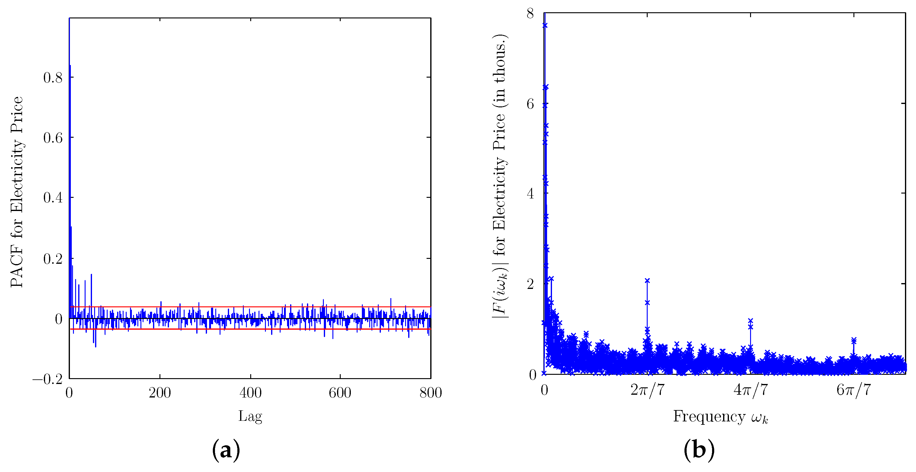
In the mean equation, $pric{e}_t$ is assumed to depend on its past values through the AR process, which allows us to take into account partial adjustment effects and seasonality features. The lags in the AR process are determined from the analysis of partial correlations summarized in Figure 2a. Volatility denoted by $h_t$ is modeled using the ARCH process. Vector $w_t$ includes the COVID-19 dummy (assumes 0 for the period before 18 March 2020 and 1 for the period from 18 March 2020), with sine and cosine periodic functions as explanatory variables. The frequencies of $2\pi /7$, $4\pi /7$, and $6\pi /7$ in the periodic functions for seasonality modeling are identified from the Fourier transform summarized in Figure 2b.

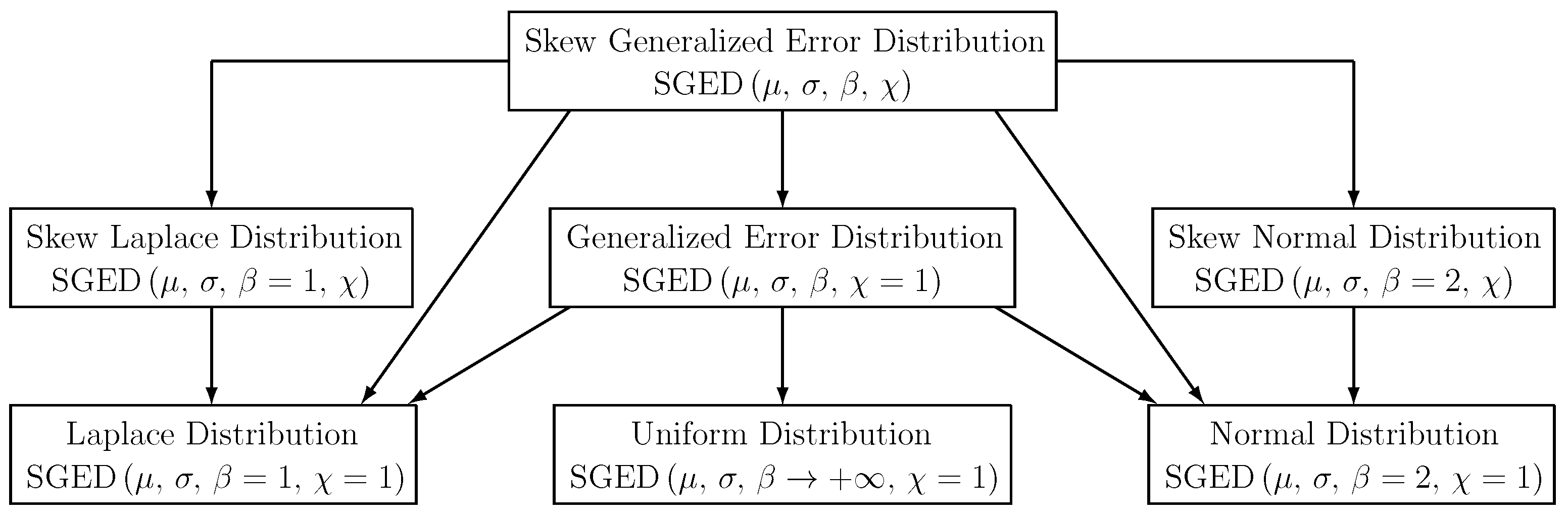
In order to jointly estimate the mean and volatility equations, we assume that standardized residuals ${\nu }_t$ defined in the third equation are independent and identically distributed (i.i.d.) and follow skew generalized error distribution (SGED). The density of SGED is defined based on [13] and depends on four parameters: mean $\mu$, standard deviation $\sigma$, shape parameter $\beta$ reflecting the peak and heavy tails, and skewness parameter $\chi$ reflecting the asymmetry. Its special cases are summarized in Figure 3.

Symmetric special cases of SGED are Laplace distribution when $\beta =1$, normal distribution when $\beta =2$, and uniform distribution when $\beta \to +\infty$. These are described in Figure 4a.

In Figure 4b, we compare normal distribution with Student’s t distribution, where the latter has heavy tails and a lower peak. Based on the illustrations in Figure 4, we suggest that using SGED may be preferred to Student’s t distribution when the data have features such as asymmetry, heavy tails, and a peak higher than in normal distribution. The distributional assumption is verified using Kullback–Leibler distance criterion.

4. Estimation Results

Most techniques in time series econometrics require stationarity of the data. Using the Augmented Dickey–Fuller (ADF) test [14], we find that the electricity price data are stationary, which allows for the application of correlograms and periodograms presented in Figure 2. These techniques are important for determining the lag structure and frequencies in the sine and cosine periodic functions. The estimation results of the AR–ARCH model assuming SGED and GED for residuals are presented in

Table 1. Estimation results when assuming SGED for standardized residuals.

Mean Equation			Volatility Equation
${\mathit{price}}_{\mathit{t}}={\mathit{a}}_{\mathbf{0}}+{\displaystyle \sum _{\mathit{i}=\mathbf{1}}^{\mathit{P}}}{\mathit{a}}_{\mathit{i}}{\mathit{price}}_{\mathit{t}-\mathit{i}}+{\mathit{w}}_{\mathit{t}}^{\prime }·\mathit{b}+{\mathit{\epsilon }}_{\mathit{t}}$			${\mathit{h}}_{\mathit{t}}={\mathit{\alpha }}_{\mathbf{0}}+{\displaystyle \sum _{\mathit{i}=\mathbf{1}}^{\mathit{p}}}{\mathit{\alpha }}_{\mathbf{i}}{\mathit{\epsilon }}_{\mathit{t}-\mathit{i}}^{\mathbf{2}}+{\mathit{w}}_{\mathit{t}}^{\prime }·\mathit{\delta }$
Variable	Coef	Std Err	Variable	Coef	Std Err
$a_0$	0.3912	0.0203	${\alpha }_0$	3.7922	0.2723
$pric{e}_{t-1}$	0.6296	0.0032	${\epsilon }_{t-1}^2$	0.3519	0.0472
$pric{e}_{t-2}$	0.0802	0.0021	${\epsilon }_{t-2}^2$	0.1500	0.0276
$pric{e}_{t-3}$	0.0438	0.0013	${\epsilon }_{t-4}^2$	0.1014	0.0273
$pric{e}_{t-4}$	0.0528	0.0016	${\epsilon }_{t-7}^2$	0.0919	0.0226
$pric{e}_{t-6}$	0.0479	0.0014	COVID-19	8.7538	2.1345
$pric{e}_{t-7}$	0.0703	0.0018	$cos(2\pi t/7)$	1.1638	0.3079
$pric{e}_{t-21}$	0.0402	0.0012
$pric{e}_{t-48}$	0.0257	0.0008
COVID-19	0.5812	0.0716
$sin(2\pi t/7)$	0.6188	0.0282
$sin(4\pi t/7)$	0.6017	0.0251
$cos(2\pi t/7)$	−0.1656	0.0208	$R^2$	0.7647
$cos(4\pi t/7)$	−0.2567	0.0203	AIC	4.9555
$cos(6\pi t/7)$	−0.4291	0.0230	MLE	−7097

Notes: All coefficient estimates are statistically significant at the 1% level. Statistically insignificant lags and periodic functions are not included.

and

Table 2. Estimation results when assuming GED for standardized residuals.

Mean Equation			Volatility Equation
${\mathit{price}}_{\mathit{t}}={\mathit{a}}_{\mathbf{0}}+{\displaystyle \sum _{\mathit{i}=\mathbf{1}}^{\mathit{P}}}{\mathit{a}}_{\mathit{i}}{\mathit{price}}_{\mathit{t}-\mathit{i}}+{\mathit{w}}_{\mathit{t}}^{\prime }·\mathit{b}+{\mathit{\epsilon }}_{\mathit{t}}$			${\mathit{h}}_{\mathit{t}}={\mathit{\alpha }}_{\mathbf{0}}+{\displaystyle \sum _{\mathit{i}=\mathbf{1}}^{\mathit{p}}}{\mathit{\alpha }}_{\mathit{i}}{\mathit{\epsilon }}_{\mathit{t}-\mathit{i}}^{\mathbf{2}}+{\mathit{w}}_{\mathit{t}}^{\prime }·\mathit{\delta }$
Variable	Coef	Std Err	Variable	Coef	Std Err
$a_0$	0.3290	0.0316	${\alpha }_0$	3.7604	0.2974
$pric{e}_{t-1}$	0.6288	0.0036	${\epsilon }_{t-1}^2$	0.3582	0.0483
$pric{e}_{t-2}$	0.0833	0.0007	${\epsilon }_{t-2}^2$	0.1500	0.0312
$pric{e}_{t-3}$	0.0353	0.0007	${\epsilon }_{t-4}^2$	0.1066	0.0289
$pric{e}_{t-4}$	0.0689	0.0008	${\epsilon }_{t-7}^2$	0.0934	0.0268
$pric{e}_{t-6}$	0.0464	0.0008	COVID-19	8.3551	2.6245
$pric{e}_{t-7}$	0.0635	0.0009	$cos(2\pi t/7)$	1.1068	0.3229
$pric{e}_{t-21}$	0.0382	0.0007
$pric{e}_{t-48}$	0.0263	0.0006
COVID-19	0.4605	0.1727
$sin(2\pi t/7)$	0.6400	0.0314
$sin(4\pi t/7)$	0.6079	0.0389
$cos(2\pi t/7)$	−0.2022	0.0297	$R^2$	0.7659
$cos(4\pi t/7)$	−0.2490	0.0276	AIC	4.9566
$cos(6\pi t/7)$	−0.4247	0.0340	MLE	−7099.7

Notes: All coefficient estimates are statistically significant at the 1% level. Statistically insignificant lags and periodic functions are not included.

, respectively.

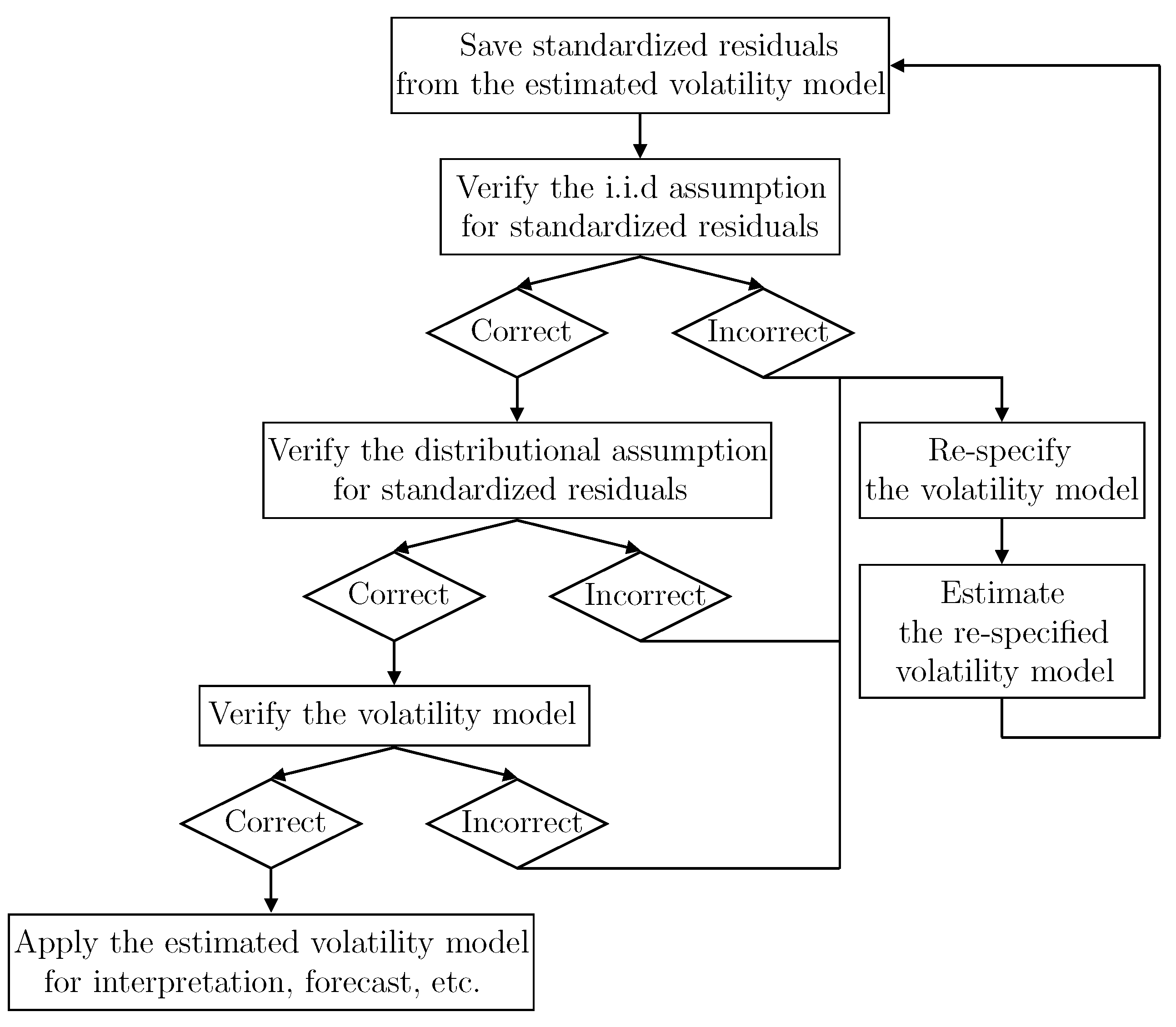
In order to be able to draw conclusions from the estimated volatility model, we must verify whether the assumptions for model residuals are satisfied. We summarize all the verification steps in Figure 5.

We first verify the assumption that the standardized residuals are independent and identically distributed (i.i.d.) using the Brock–Dechert–Scheinkman test (BDS test) further developed in [15]. The test results are presented in

Table 3. BDS test for standardized residuals when assuming SGED.

Dimension	BDS Test	p-Value	BDS Test	p-Value
2	0.0006	0.6900	0.0021	0.4183
3	−0.0015	0.5662	−0.0009	0.8317
4	−0.0005	0.8709	0.0004	0.9357
5	−0.0003	0.9200	0.0004	0.9470
6	0.0011	0.7215	0.0025	0.6251
	$H_0:{\nu }_t$ is i.i.d.		$H_0:{\nu }_t^2$ is i.i.d.

. The null hypotheses are not rejected because the p-values are greater than 10%. Not rejecting ${\nu }_t$ being i.i.d. suggests that ${\nu }_t$ is not serially correlated. Similarly, not rejecting ${\nu }_t^2$ being i.i.d. suggests that ${\nu }_t$ is not heteroscedastic. Therefore, we conclude that the residuals do not contain any information and are random.

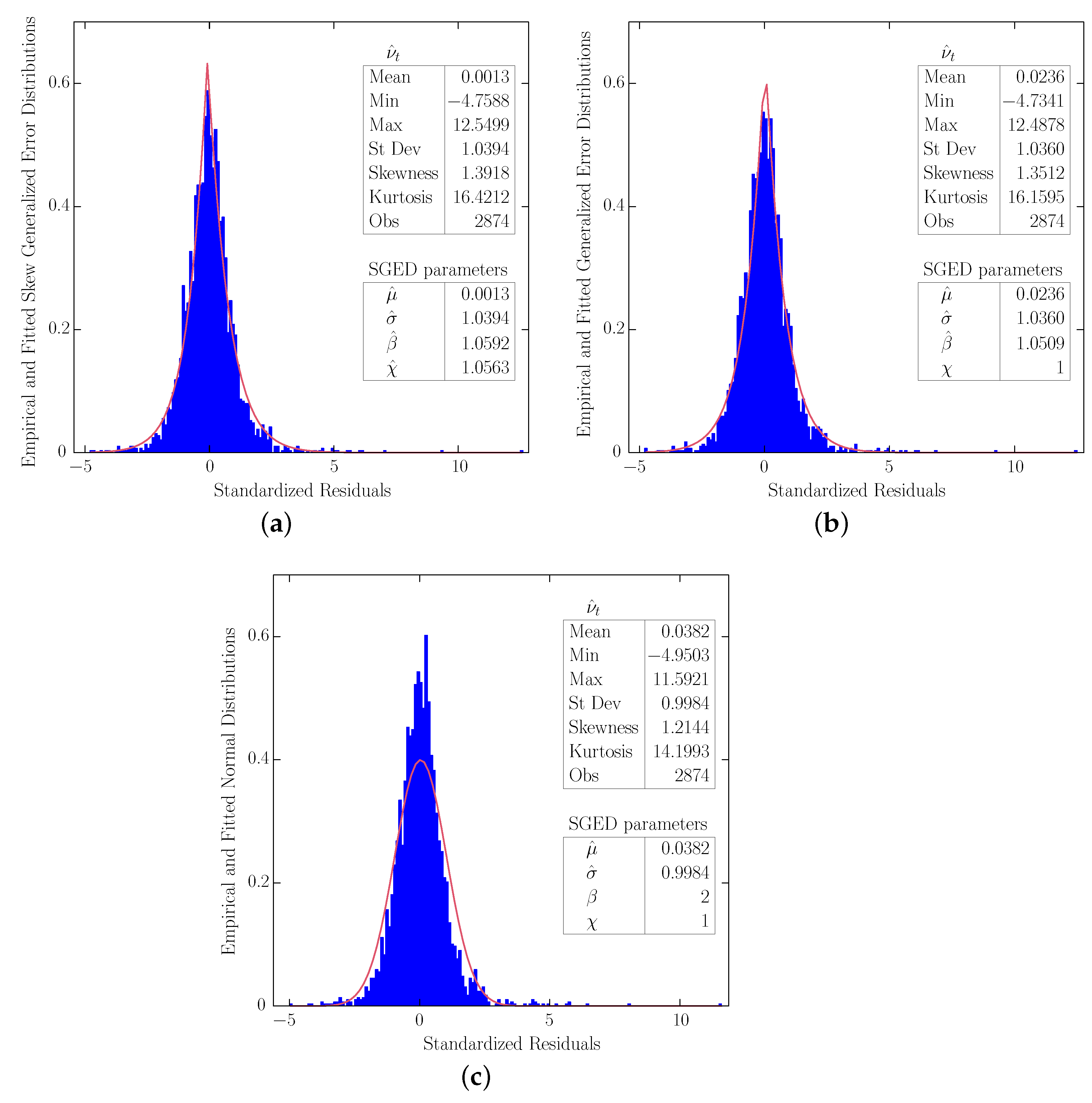
The next verification step is related to the distributional assumption. We estimated three volatility models, assuming that standardized residuals follow skew generalized error distribution (SGED), generalized error distribution (GED), and normal distribution. In Figure 6a–c, we compare the empirical distributions of model residuals with the fitted SGED, GED, and normal distribution, respectively. The fitted SGED and GED in Figure 6a,b provide a far better match for the empirical distribution of standardized residuals than the fitted normal distribution in Figure 6c. That is why we presented only estimation results assuming SGED and GED for model residuals.

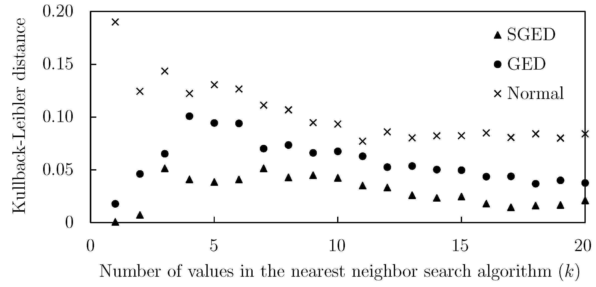
Comparing SGED and GED is more difficult. For assessment, we use the Kullback–Leibler distance, which allows us to determine how close an empirical distribution is to a theoretical probability distribution [16]. The results presented in

Table 4. Kullback–Leibler distance for empirical and fitted theoretical distributions of standardized residuals.

	Assumed Distributions
k	SGED	GED	Normal
1	0.0006	0.0177	0.1901
2	0.0071	0.0461	0.1244
3	0.0513	0.0652	0.1436
4	0.0409	0.1008	0.1223
5	0.0384	0.0944	0.1306
6	0.0408	0.0940	0.1265
7	0.0513	0.0701	0.1113
8	0.0428	0.0734	0.1067
9	0.0449	0.0661	0.0947
10	0.0423	0.0675	0.0933
11	0.0350	0.0628	0.0770
12	0.0331	0.0525	0.0859
13	0.0259	0.0535	0.0803
14	0.0233	0.0502	0.0822
15	0.0247	0.0496	0.0823
16	0.0180	0.0435	0.0850
17	0.0144	0.0438	0.0806
18	0.0160	0.0369	0.0840
19	0.0167	0.0401	0.0800
20	0.0210	0.0375	0.0841

Notes: k is the number of values in the nearest neighbor search algorithm. The default number of values is usually set equal to 10.

and Figure 7 indicate that the Kullback–Leibler distance between the empirical and fitted theoretical distributions of the standardized residuals is smaller under the SGED assumption, which suggests that the SGED assumption is the most appropriate.

As presented in

Table 5. Akaike information criterion (AIC) and log-likelihood function from three volatility models when assuming SGED, GED, and normal distribution for standardized residuals.

Assumed Distributions	SGED	GED	Normal
SGED Parameters	$(\mathit{\mu },\mathit{\sigma },\mathit{\beta },\mathit{\chi })$	$(\mathit{\mu },\mathit{\sigma },\mathit{\beta },\mathit{\chi }=1)$	$(\mathit{\mu },\mathit{\sigma },\mathit{\beta }=2,\mathit{\chi }=1)$
AIC	4.9555	4.9566	5.1409
Log-likelihood function	−7097.0	−7099.7	−7365.5

Notes: GED is a special case of SGED when χ = 1. Similarly, normal distribution is a special case of SGED when β = 2 and χ = 1. These details are summarized in Figure 3.

, under the SGED assumption, the value of the Akaike information criterion (AIC) is lower and the value of the log-likelihood function is higher. On the one hand, a lower value of the AIC suggests that less information is lost, hence a higher quality of the chosen volatility model. On the other hand, a higher value of the log-likelihood function suggests that the chosen volatility model is more likely to produce prices that were actually observed. Therefore, we conclude that the SGED assumption reflecting asymmetry, a higher peak, and heavy tails is correct for our volatility model.

Even if both distributional assumptions are satisfied (the i.i.d. and SGED), the overall volatility model may be incorrect due to possible remaining asymmetries. This is the last third verification step presented in Figure 5. We verify if the overall conditional volatility model is specified correctly using the sign-bias test presented in

Table 6. t-test values of the sign bias test for standardized residuals.

	t-Test	p-Value
Sign Bias	1.48	0.14
Negative Sign Bias	0.06	0.95
Positive Sign Bias	0.46	0.65
Joint Effect	2.76	0.43

. Because all p-values are above 10%, we conclude that the volatility model is correctly specified.

5. Discussion

According to [17], understanding the volatility dynamics of electricity markets is important in evaluating the deregulation experience, in forecasting, and in pricing electricity futures and other energy derivatives. Modelling price volatility is also needed to build accurate pricing models; to forecast future price volatility; and to enrich our understanding of the broader financial markets, the energy industry, and the overall economy [18]. Therefore, modeling the dynamics of electricity prices and volatility is of a primary interest for investors, producers, and policymakers.

We find that the empirical distribution of electricity prices is asymmetric, and has heavy tails and a peak higher than in the fitted normal distribution. These observations suggest that we can assume SGED for model residuals. We show the correctness of our distributional assumptions and the volatility model using various tests and criteria.

Some papers however do not discuss the empirical distribution of model residuals in order to verify the distributional assumptions (an i.i.d. and an assumed theoretical distribution). For example, most of the GARCH-type estimated models presented in Tables 3–6 from [7] violated no serial correlation assumption for standardized residuals or standardized residuals squared.

Most frequently assumed distributions are normal, Student’s t, and GED. Reference [19] applied a GARCH model assuming those distributions in modeling crude oil prices. The research finds that Student’s t distribution is superior due to the extremely high kurtosis in oil return volatility. The peak of the empirical distribution of residuals compared to the fitted normal distribution is however not discussed. Heavy tails and high kurtosis can be modeled using GED or Student’s t distribution depending on the peak being higher or lower than in the fitted normal distribution, as described in Figure 4.

Reference [20] suggests that replacing the normality assumption with a heavy-tailed distribution might improve the forecast results. Indeed, when assuming SGED, we find that the value of the log-likelihood function was the highest compared to GED and normal distribution (Table 5). However, normal distribution is still used frequently (e.g., [21,22]) even when there is ample evidence that data or model residuals do not follow normal distribution [23].

Correctly specified volatility models can be applied for forecast or interpretation of changes due to reforms or other events. We proceed to the analysis of the possible effect of the COVID-19 pandemic on price level and volatility. For this purpose, we consider the COVID-19 dummy variable, which is equal to 0 for the period before 18 March 2020 and is equal to 1 for the period from 18 March 2020. As presented in Table 1, the coefficient estimates in front of the COVID-19 dummy variable in the mean and volatility equations are positive and statistically significant. This suggests that, on average, the price level and volatility increased during the pandemic.

6. Conclusions

Verifying all assumptions in volatility modeling is crucial for the later application of models in forecasting, policy evaluation, or analysis of the impact of various events. When an empirical distribution of data has features such as asymmetry, heavy tails, and a peak higher than in the fitted normal distribution, then we suggest assuming SGED for model residuals. This suggestion is supported by our findings of asymmetry (a positive skewness coefficient and a skewness parameter above one) and excess kurtosis (kurtosis above three) presented in Figure 6. Moreover, when assuming SGED for model residuals, we obtain a lower value of AIC and a higher value of the log-likelihood function (Table 5). Hence, we conclude that considering SGED including GED or normal distribution as its special cases can allow for more accurate modeling.

Given a correctly specified volatility model, it is possible to test various hypotheses. In our case, we test if the COVID-19 pandemic affected price level and volatility. We find that both price level and volatility increased after the start of the COVID-19 pandemic.

We had to limit our study to the period until 31 December 2020 because this is the time when the Brexit transition period ended. Current changes in 2021 in the price level and volatility could be related to Brexit, too. It may be necessary to analyze a longer time horizon after the pandemic is over in order to decompose the change due to the pandemic or Brexit. Then, it may be possible to evaluate the impact of Brexit on price level and volatility after its transition period ended on 31 December 2020.

The suggested extension would however require an introduction of another dummy variable for the Brexit analysis. This should not be an issue if seasonality of data is modeled using periodic functions based on the Fourier transform presented in Figure 2b. Periodic functions may allow us to specify a parsimonious model compared to when using day of the week dummy variables in modeling weekly seasonality. Then, dummy variables could be used for analysis of the effect of various events.

References

- Wan, K.W. Nasdaq, Nord Pool Launch New UK Power Market. 2010. Available online: https://www.reuters.com/article/idUSLDE60B27120100112?edition-redirect=uk (accessed on 15 December 2020).
- Engle, R.F. Autoregressive conditional heteroscedasticity with estimates of the variance of United Kingdom inflation. Econometrica 1982, 50, 987–1007. [Google Scholar] [CrossRef]
- Bollerslev, T. Generalized autoregressive conditional heteroscedasticity. J. Econom. 1986, 31, 307–327. [Google Scholar] [CrossRef] [Green Version]
- Nelson, D.B. Conditional heteroskedasticity in asset returns: A new approach. Econometrica 1991, 59, 347–370. [Google Scholar] [CrossRef]
- Ciarreta, A.; Zarraga, A. Modeling realized volatility on the Spanish intra-day electricity market. Energy Econ. 2016, 58, 152–163. [Google Scholar] [CrossRef]
- Charles, A.; Darné, O. Forecasting crude-oil market volatility: Further evidence with jumps. Energy Econ. 2017, 67, 508–519. [Google Scholar] [CrossRef]
- Zhang, Y.J.; Yao, T.; Ripple, R. Volatility forecasting of crude oil market: Can the regime switching GARCH model beat the single-regime GARCH models? Int. Rev. Econ. Financ. 2019, 59, 302–317. [Google Scholar] [CrossRef]
- Lin, Y.; Xiao, Y.; Li, F. Forecasting crude oil price volatility via a HM-EGARCH model. Energy Econ. 2020, 87, 1–13. [Google Scholar] [CrossRef]
- Koopman, S.J.; Ooms, M.; Carnero, M.A. Periodic seasonal Reg-ARFIMA-GARCH models for daily electricity spot prices. J. Am. Stat. Assoc. 2007, 102, 16–27. [Google Scholar] [CrossRef] [Green Version]
- Lee, Y.H.; Pai, T.Y. REIT volatility prediction for skew-GED distribution of the GARCH model. Expert Syst. Appl. 2010, 37, 4737–4741. [Google Scholar] [CrossRef]
- Su, J.B. How to mitigate the impact of inappropriate distributional settings when the parametric value-at-risk approach is used. Quant. Financ. 2014, 14, 305–325. [Google Scholar] [CrossRef]
- Tashpulatov, S.N. The impact of behavioral and structural remedies on electricity prices: The case of the England and Wales electricity market. Energies 2018, 11, 3420. [Google Scholar] [CrossRef] [Green Version]
- Fernández, C.; Steel, M. On Bayesian modeling of fat tails and skewness. J. Am. Stat. Assoc. 1998, 93, 359–371. [Google Scholar]
- Dickey, D.A.; Fuller, W.A. Likelihood ratio statistics for autoregressive time series with a unit root. Econometrica 1981, 49, 1057–1072. [Google Scholar] [CrossRef]
- Brock, W.A.; Dechert, W.D.; Scheinkman, J.A.; LeBaron, B. A test for independence based on the correlation dimension. Econom. Rev. 1996, 15, 197–235. [Google Scholar] [CrossRef]
- Kullback, S.; Leibler, R.A. On information and sufficiency. Ann. Math. Stat. 1951, 22, 79–86. [Google Scholar] [CrossRef]
- Hadsell, L.; Marathe, A.; Shawky, H.A. Estimating the volatility of wholesale electricity spot prices in the US. Energy J. 2004, 25, 23–40. [Google Scholar] [CrossRef] [Green Version]
- Ewing, B.; Malik, F. Modelling asymmetric volatility in oil prices under structural breaks. Energy Econ. 2017, 63, 227–233. [Google Scholar] [CrossRef]
- Herrera, A.M.; Hu, L.; Pastor, D. Food price volatility and macroeconomic factors: Evidence from GARCH and GARCH-X estimates. Int. J. Forecast. 2018, 34, 622–635. [Google Scholar] [CrossRef]
- Shen, Z.; Ritte, M. Forecasting volatility of wind power production. Appl. Energy 2016, 176, 295–308. [Google Scholar] [CrossRef] [Green Version]
- Ergen, I.; Rizvanoghlu, I. Asymmetric impacts of fundamentals on the natural gas futures volatility: An augmented GARCH approach. Energy Econ. 2016, 56, 64–74. [Google Scholar] [CrossRef]
- Nonejad, N. Crude oil price volatility and equity return predictability: A comparative out-of-sample study. Int. Rev. Financ. Anal. 2020, 71, 1–18. [Google Scholar] [CrossRef]
- Shalini, V.; Prasanna, K. Impact of the financial crisis on Indian commodity markets: Structural breaks and volatility dynamics. Energy Econ. 2016, 53, 40–57. [Google Scholar] [CrossRef]
Figure 1.
Electricity prices on the N2EX market during 1 January 2013–31 December 2020. Source: https://www.nordpoolgroup.com/, accessed on 1 January 2021. Author’s calculations.
Figure 2.
Analysis of partial correlations and periodogram for electricity prices. Source: Author’s calculations.
Figure 3.
All special cases of skew generalized error distribution SGED . Source: Author’s illustration.
Figure 4.
SGED and Student’s t distribution. Notes: In (a), we show three special cases of SGED: Laplace distribution (black) when , standard normal distribution (red) when , and uniform distribution (green) when . Generally, if , then the distribution is leptokurtic, with heavier tails and a peak more acute and higher than in normal distribution. In (b), we compare normal distribution with Student’s t distribution. As the number of degrees of freedom increases, Student’s t distribution approaches normal distribution. (a) Special cases of SGED; (b) normal and Student’s t distributions. Source: Author’s illustration.
Figure 5.
Model selection scheme. Source: Author’s illustration.
Figure 6.
Empirical and fitted theoretical distributions of standardized residuals . Notes: GED is a special case of SGED when . Similarly, normal distribution is a special case of SGED when and . These details are summarized in Figure 3.
Figure 7.
Illustration of the values of the Kullback–Leibler distance based on Table 4.