Multigrid Method for Optimal Control Problem Constrained by Stochastic Stokes Equations with Noise

Abstract

Optimal control problems governed by stochastic partial differential equations have become an important field in applied mathematics. In this article, we investigate one such important optimization problem, that is, the stochastic Stokes control problem with forcing term perturbed by noise. A multigrid scheme with three-factor coarsening to solve the corresponding discretized control problem is presented. On staggered grids, a three-factor coarsening strategy helps in simplifying the inter-grid transfer operators and reduction in computation (CPU time). For smoothing, a distributive Gauss–Seidel scheme with a line search strategy is employed. To validate the proposed multigrid staggered grid framework, numerical results are presented with white noise at the end.

1. Introduction

Optimal control problems governed by partial differential equations (PDEs) have been studied extensively for the last three decades [1,2]. Particularly, control problem constrined by Stokes and/or Navier–Stokes equations play an important role in many real-world applications such as data assimilation for ocean flows, weather models, and flow problems. Recently, there has been a growing interest in mathematical analysis and simulations of stochastic PDEs (e.g., see [3,4,5,6,7,8]). The motivation of our work is the stochastic optimal control problem with PDEs as constraints (with random inputs) (see [8,9,10,11] and the references therein).

Multigrid methods are the well known efficient schemes to solve the elliptic boundary value problems [12,13,14]. However, to solve the saddle point problems such as the Stokes equations (after discretization with finite differences or finite element), the multigrid methods are more involved [15,16]. The multigrid methods have also been investigated for the flow problems [17,18,19,20,21,22,23,24]. Moreover, there has already been a lot of work on the multigrid solvers for the optimal control problems governed by PDEs in literature (e.g., see [25]).

This paper investigates a multigrid algorithm that solves the (finite difference) discretized optimality system corresponding to the control problem governed by stochastic Stokes equations (with force driven by additive white noise). In particular, we propose a full multigrid method with three-factor coarsening strategy to solve numerically the distributed optimal control problem constrained by stochastic Stokes equations (driven by the white noise perturbed forcing term). The scope of this paper is to develop an efficient multigrid algorithm without the need of any preconditioner [26], which results in fewer computations (CPU time) for the control problems with stochastic models, such as the one in [8]. For this, we take advantage of our previous works on multigrid methods for distributed optimal control problem governed by Stokes equations [27,28].

The objective of the proposed control formulation is to seek a state and a control that minimize the expectation of the distances between the approximate and desired state. In particular, the target state and the control are deterministic. The main difference between the present study and earlier research is the additive white noise in the forcing term that derives the stochastic Stokes equations. Therefore, we need to discretize the noise and modify the whole multigrid scheme for the optimization problem (stochastic model optimization) accordingly, which is explained in this article.

The paper is organized as follows. In next section. the control problem constrained by the stochastic Stokes equations is presented and first-order optimality conditions are discussed. On staggered grids, finite difference approximations are used to discretize the optimality system in Section 3. In Section 4, the proposed full multigrid method with smoothing and intergrid transfer operators (prolongation and restriction) is explained. In Section 5, numerical experiments for the control problem and stochastic Stokes equations with additive white noise are presented. In the end, the conclusions are given.

2. The Control Problem

We consider the following control problem in a convex polygon domain $\mathsf{\Omega }\subset {\mathbb{R}}^2$ with boundary $\Gamma =\partial \mathsf{\Omega }$: Given a white noise $\dot{\mathbf{W}}$ and a target function $\mathbf{U}$, find an optimal stochastic state $\mathbf{u}\in {\mathbf{H}}^1\left(\mathsf{\Omega }\right)$ and a control $\mathbf{f}\in {\mathbf{L}}^2\left(\mathsf{\Omega }\right)$ while the deterministic cost functional is minimized, i.e.,

$$\mathrm{Min}J(\mathbf{u},\mathbf{f}):=\mathbb{E}\left[\frac{1}{2}{\int }_{\mathsf{\Omega }}{|\mathbf{u}-\mathbf{U}|}^{2}dx\right]+\frac{\alpha }{2}{\int }_{\mathsf{\Omega }}{\left|\mathbf{f}\right|}^{2}dx$$

(1)

subject to stochastic Stokes equations:

$$\begin{array}{ccc}\hfill -\nu ▵\mathbf{u}+\nabla p& =& \mathbf{f}+\sigma \dot{\mathbf{W}},\mathrm{in}\mathsf{\Omega }\hfill \end{array}$$

(2)

$$\begin{array}{ccc}\hfill -\nabla ·\mathbf{u}& =& 0,\mathrm{in}\mathsf{\Omega }\hfill \end{array}$$

(3)

$$\begin{array}{ccc}\hfill \mathbf{u}& =& 0,\mathrm{on}\Gamma .\hfill \end{array}$$

(4)

We denote $p\in L^2\left(\mathsf{\Omega }\right)$ a pressure, $\mathbf{f}$ a control, and $\mathbf{U}\in {\mathbf{L}}^2\left(\mathsf{\Omega }\right)$ the desired velocity. Moreover, $\nu$ is a viscous constant, $\sigma$ is a positive continuous function in $\mathsf{\Omega }$, $\alpha >0$ is the weight of the cost of control, $\dot{\mathbf{W}}=({\dot{W}}^1,{\dot{W}}^2)$ is the white noise, and

$$\mathbb{E}\left[{\dot{W}}^j\left(x\right){\dot{W}}^j\left(x^{\prime }\right)\right]=\delta (x-x^{\prime }),x,x^{\prime }\in \mathsf{\Omega }.$$

We additionally assume that ${\int }_{\mathsf{\Omega }}pdx=0$, that is, p satisfies the zero mean constraint. Furthermore, we denote $\mathbf{u}={(u_1,\dots ,u_n)}^T\in {\mathbb{R}}^n$, $\left|\mathbf{u}\right|=\sqrt{u_1^2,\dots ,u_n^2}$, unless otherwise stated.

We denote the inner product associated with Lebesque space $L^2\left(\mathsf{\Omega }\right)$ by $(·,·)$ and

$$\begin{array}{c}\hfill L_0^2\left(\mathsf{\Omega }\right)=\left\{\varphi \in L^2\left(\mathsf{\Omega }\right):{\int }_{\mathsf{\Omega }}\varphi dx=0\right\},\\ \hfill {\mathbf{H}}_0^1\left(\mathsf{\Omega }\right)=\left\{\psi \in {\mathbf{H}}^1\left(\mathsf{\Omega }\right):\psi =0\mathrm{on}\partial \mathsf{\Omega }\right\}.\end{array}$$

The weak solution $(\mathbf{u},p)\in {\mathbf{H}}_0^1\left(\mathsf{\Omega }\right)\times L_0^2\left(\mathsf{\Omega }\right)$ of (2)–(4) is the solution of

$$\begin{array}{ccc}\hfill \nu a(\mathbf{u},\mathbf{w})+b(\mathbf{w},p)& =& (\mathbf{f},\mathbf{w})+(\sigma \dot{\mathbf{W}},\mathbf{w})\forall \mathbf{w}\in {\mathbf{H}}_0^1\left(\mathsf{\Omega }\right)\hfill \\ \hfill b(\mathbf{u},\psi )& =& 0\forall \psi \in L_0^2\left(\mathsf{\Omega }\right),\hfill \end{array}$$

where we denote $a:{\mathbf{H}}_0^1\left(\mathsf{\Omega }\right)\times {\mathbf{H}}_0^1\left(\mathsf{\Omega }\right)\to \mathbb{R}$ and $b:{\mathbf{H}}_0^1\left(\mathsf{\Omega }\right)\times L_0^2\left(\mathsf{\Omega }\right)$ as the bilinear forms, i.e.,

$$\begin{array}{ccc}\hfill a(\mathbf{u},\mathbf{w})& =& \sum _{j=1}^2{\int }_{\mathsf{\Omega }}\nabla {\mathbf{u}}_j·\nabla {\mathbf{w}}_j\hfill \\ \hfill b(\mathbf{w},p)& =& -{\int }_{\mathsf{\Omega }}p\nabla ·\mathbf{w}\hfill \end{array}$$

The existence and uniqueness of the control problem can easily be proven by following the standard arguments (see [1,29]). We define the set of admissible controls

$${\mathbf{F}}_{ad}=\{(\mathbf{u},p,\mathbf{f})\in {\mathbf{H}}_0^1\left(\mathsf{\Omega }\right)\times L_0^2\left(\mathsf{\Omega }\right)\times {\mathbf{L}}^2\left(\mathsf{\Omega }\right):\widehat{J}\left(\mathbf{f}\right)=J(\mathbf{u},p,\mathbf{f})<\infty ;(\mathbf{u},p,\mathbf{f})\mathrm{satisfies}\left(2\right)-\left(3\right)\}$$

The optimal solution $({\mathbf{u}}^{*},p^{*},{\mathbf{f}}^{*})\in \mathbf{F}$ is such that if there exists a $\epsilon >0$ such that

$$J({\mathbf{u}}^{*},p^{*},{\mathbf{f}}^{*})\le J(\mathbf{u},p,\mathbf{f})\forall (\mathbf{u},p,\mathbf{f})\in {\mathbf{F}}_{ad}$$

and

$$\parallel {\mathbf{u}}^{*}{-\mathbf{u}\parallel }_2+\parallel p^{*}{-p\parallel }_{-1}+{\parallel {\mathbf{f}}^{*}-\mathbf{f}\parallel }_2\le \epsilon$$

Now, we can formulate the optimal control problem that seeks $(\mathbf{u},p,\mathbf{f})$ that minimize the cost functional (1) subject to (2)–(3), i.e.,

$$\min J(\mathbf{u},p,\mathbf{f})$$

(5)

as a constrained optimization problem with (2)–(3) in Hilbert space such that $(\mathbf{u},p,\mathbf{f})\in {\mathbf{F}}_{ad}$. In the following, we present the first-order optimality conditions for completeness:

Theorem 1.

The optimization problem (5) has a unique solution $({\mathbf{u}}^{*},p^{*},{\mathbf{f}}^{*})\in {\mathbf{F}}_{ad}$.

Proof. 

Since ${\mathbf{F}}_{ad}$ is not empty, for example, $(\mathbf{u},p,\mathbf{0})\in {\mathbf{F}}_{ad}$.

Let ${\mathbf{f}}_n$ be a minimizing sequence and set the linear dependency of control to state variables as ${\mathbf{u}}_n=\mathbf{u}\left({\mathbf{f}}_n\right)$ and $p_n=p\left({\mathbf{u}}_n\right)$. Moreover,

$${\lim }_{n\to \infty }J({\mathbf{u}}_n,p_n,{\mathbf{f}}_n)=\inf J(\mathbf{u},p,\mathbf{f})$$

By definition of ${\mathbf{F}}_{ad}$, the sequence ${\mathbf{f}}_n$ is uniformly bounded in ${\mathbf{L}}^2\left(\mathsf{\Omega }\right)$. From the weak solutions to state system, we conclude that the sequence $({\mathbf{u}}_n,p_n)$ is uniformly bounded in ${\mathbf{L}}^2\left(\mathsf{\Omega }\right)\times H_0^1\left(\mathsf{\Omega }\right)$ almost surely. Thus, we have a subsequence $({\mathbf{u}}_l,p_l,{\mathbf{f}}_l)$ such that

$${\mathbf{f}}_l\rightharpoonup {\mathbf{f}}^{*},p_l\rightharpoonup p^{*},{\mathbf{u}}_l\rightharpoonup {\mathbf{u}}^{*}$$

for some $({\mathbf{u}}^{*},p^{*},{\mathbf{f}}^{*})\in {\mathbf{L}}^2\left(\mathsf{\Omega }\right)\times H_0^1\left(\mathsf{\Omega }\right)\times {\mathbf{L}}^2\left(\mathsf{\Omega }\right)$.

Next, by the weak lower semi-continuity of the cost functional J, we have

$$\inf J({\mathbf{u}}_n,p_n,{\mathbf{f}}_n)={\lim }_{n\to \infty }J({\mathbf{u}}_n,p_n,{\mathbf{f}}_n)=J({\mathbf{u}}^{*},p^{*},{\mathbf{f}}^{*})$$

Hence, we see that the optimal solution (in the set ${\mathbf{F}}_{ad}$) exists. Next, to prove that this optimal solution is unique, we use the fact that the constraints are linear and the cost functional is convex. This completes the proof. □

Next, the solution to the control problem (1)–(4) is characterized by the Lagrangian [1,30]. That is, the first-order optimality conditions for the (stochastic Stokes equations) optimization problem is obtained by taking the Gâteaux (Fréchet) derivative of the following Lagrangian functional

$$L(\mathbf{u},\mathbf{f},p,\lambda ,q)=J(\mathbf{u},\mathbf{f})+(-\Delta \mathbf{u}+\nabla p-\mathbf{f}-\sigma \dot{\mathbf{W}},\lambda )-(\nabla ·\mathbf{u},q),$$

where we denote the Lagrange multipliers $\lambda \in {\mathbf{H}}_0^1\left(\mathsf{\Omega }\right)$, $q\in L_0^2\left(\mathsf{\Omega }\right)$. Thus, we have the optimality system given by [8]:

$$\begin{array}{ccc}\hfill -\nu \Delta \mathbf{u}+\nabla p& =& \mathbf{f}+\sigma \dot{\mathbf{W}}\mathrm{in}\mathsf{\Omega },\hfill \\ \hfill -\nabla ·\mathbf{u}& =& 0\mathrm{in}\mathsf{\Omega }\left(\mathrm{state}\mathrm{system}\right)\hfill \\ \hfill \mathbf{u}& =& 0\mathrm{on}\Gamma ,\hfill \end{array}$$

(6)

$$\begin{array}{ccc}\hfill -\Delta \lambda +\nabla q& =& \mathbf{U}-\mathbf{u}\mathrm{in}\mathsf{\Omega }\hfill \\ \hfill -\nabla ·\lambda & =& 0\mathrm{in}\mathsf{\Omega }\left(\mathrm{adjoint}\mathrm{system}\right)\hfill \\ \hfill \lambda & =& 0\mathrm{on}\Gamma ,\hfill \end{array}$$

(7)

$$\begin{array}{ccc}\hfill \alpha \mathbf{f}-\mathbb{E}\left[\lambda \right]& =& 0\mathrm{in}\mathsf{\Omega },\left(\mathrm{optimality}\mathrm{conditions}\right)\hfill \end{array}$$

(8)

where $\nabla ·\mathbf{u}=\mathrm{div}\mathbf{u},\nabla p=\mathrm{grad}p$, $\mathbf{u}=(u,v),\lambda =(\lambda ,\mu )$, etc.

From the optimality conditions, we have that $\mathbf{f}=\frac{\mathbb{E}\left[\lambda \right]}{\alpha }$. Therefore, we can write the above optimality system into a reduced optimality system as follows, i.e., we find $(\mathbf{u},p,\lambda ,q)$ while satisfying the following system:

$$\begin{array}{ccc}\hfill -\Delta \mathbf{u}+\nabla p& =& \frac{\mathbb{E}\left[\lambda \right]}{\alpha }+\dot{\mathbf{W}}\mathrm{in}\mathsf{\Omega },-\nabla ·\mathbf{u}=0\mathrm{in}\mathsf{\Omega },\mathbf{u}=0\mathrm{on}\Gamma ,\hfill \\ \hfill -\Delta \lambda +\nabla q& =& \mathbf{U}-\mathbf{u}\mathrm{in}\mathsf{\Omega },-\nabla ·\lambda =0\mathrm{in}\mathsf{\Omega },\lambda =0\mathrm{on}\Gamma ,\hfill \\ \hfill \alpha \mathbf{f}-\mathbb{E}\left[\lambda \right]& =& 0\mathrm{in}\mathsf{\Omega }.\hfill \end{array}$$

(9)

3. Discretization

In the following, we discretize the optimality system using finite differences on staggered grids. For this, we first discretize the white noise $\dot{\mathbf{W}}$. Let $\left\{{\mathcal{R}}_h\right\}$ be a family of rectangles $\overline{\mathsf{\Omega }}$, where h is the mesh size. Define

$${\xi }_R^j=\frac{1}{\sqrt{\left|R\right|}}{\int }_{R}1d{W}^j,j=1,2$$

(10)

for each rectangle $R\in {\mathcal{R}}_h$, and $\left|R\right|$ is the area of R. Here and in what follows, ${\xi }_{R\in \mathcal{R}}^j$ denotes an independent distributed normal random variables family, i.e., with the mean 0 and variance 1. The piecewise constant approximation to ${\dot{W}}^j\left(x\right)$ is defined as follows

$${\dot{W}}_h^j\left(x\right)=\sum _{R\in {\mathcal{R}}_h}\frac{1}{\sqrt{\left|R\right|}}{\xi }_R^j{\chi }_R\left(x\right),$$

(11)

where ${\chi }_R$ is the characteristic function of R. Moreover, $\dot{\mathbf{W}}=({\dot{W}}_h^1,{\dot{W}}_h^2)\in {\left(L^2\left(\mathsf{\Omega }\right)\right)}^2$ but $\parallel {\dot{\mathbf{W}}}_h\parallel$ is unbounded as $h\to 0$ (see Lemma 1.2 [8]).

Next, we consider the approximation problem (2)–(4) with the discrete white noise forcing term:

$$\begin{array}{ccc}\hfill -\nu ▵{\mathbf{u}}_h+\nabla p_h& =& {\mathbf{f}}_h+\sigma {\dot{\mathbf{W}}}_h,\mathrm{in}\mathsf{\Omega }\hfill \end{array}$$

(12)

$$\begin{array}{ccc}\hfill -\nabla ·{\mathbf{u}}_h& =& 0,\mathrm{in}\mathsf{\Omega }\hfill \end{array}$$

(13)

$$\begin{array}{ccc}\hfill {\mathbf{u}}_h& =& 0,\mathrm{on}\Gamma .\hfill \end{array}$$

(14)

Then, by Choi and Lee [8], we have the following estimates (for ${\mathbf{u}}_h$ and $p_h$, where h is the mesh size):

Proposition 1.

$\mathbb{E}\left[\parallel {\mathbf{u}}_h{\parallel }_2^2+{\parallel p_h\parallel }_1^2\right]\le C{h}^{-2}$

and for errors $\mathbf{u}-{\mathbf{u}}_h$ and $p-p_h$:

Proposition 2.

$\mathbb{E}\left[\parallel \mathbf{u}-{\mathbf{u}}_h{\parallel }^2+{\parallel p-p_h\parallel }_{-1}^2\right]\le C\left|lnh\right|h^2$.

Next, we consider a sequence of grids ${\left\{{\mathsf{\Omega }}_h\right\}}_{h>0}$ for a rectangular domain $\mathsf{\Omega }$ given by

$${\mathsf{\Omega }}_h=\{\mathbf{x}\in {\mathbb{R}}^2:x_i=i{h}_x,y_j=j{h}_y,i,j\in \mathbb{Z}\}\cap \mathsf{\Omega },$$

Here and in what follows, we take the mesh size ($h_x=h_y=h$) and choose h in such a way that the boundaries of $\mathsf{\Omega }$ lie on the grid lines.

Note that, on the staggered grids, the state (respectively, adjoint) variables are placed on cell edges (vertical or horizontal) and on cell centers. We denote these sets of grid points with ${\mathsf{\Omega }}_h^s$, $s\in \{ev,eh,c\}$. For example, ${\mathsf{\Omega }}_h^{ev}$ denotes the grid points defined on center of cell edge-vertical. Moreover, the discrete $L^2$-scalar product is given by

$${(u^h,v^h)}_{L_h^2\left({\mathsf{\Omega }}_h^s\right)}=h_x{h}_y\sum _{\mathbf{x}\in {\mathsf{\Omega }}_h^s}{u}^h\left(\mathbf{x}\right)v^h\left(\mathbf{x}\right),$$

and the associated norm is given by $\parallel u^h{\parallel }_{L_h^2\left({\mathsf{\Omega }}_h^s\right)}={(u^h,u^h)}_{L_h^2\left({\mathsf{\Omega }}_h^s\right)}^{1/2}$. Let $L_h^2\left({\mathsf{\Omega }}_h^s\right)$ be the grid of grid functions $u^h$ defined on ${\mathsf{\Omega }}_h^s$. Moreover, we denote ${\mathcal{U}}_h$, ${\mathcal{V}}_h$ and ${\mathcal{P}}_h$ the spaces for the state (respectively, adjoint) grid functions variables $u^h$, $v^h$, and $p^h$, respectively.

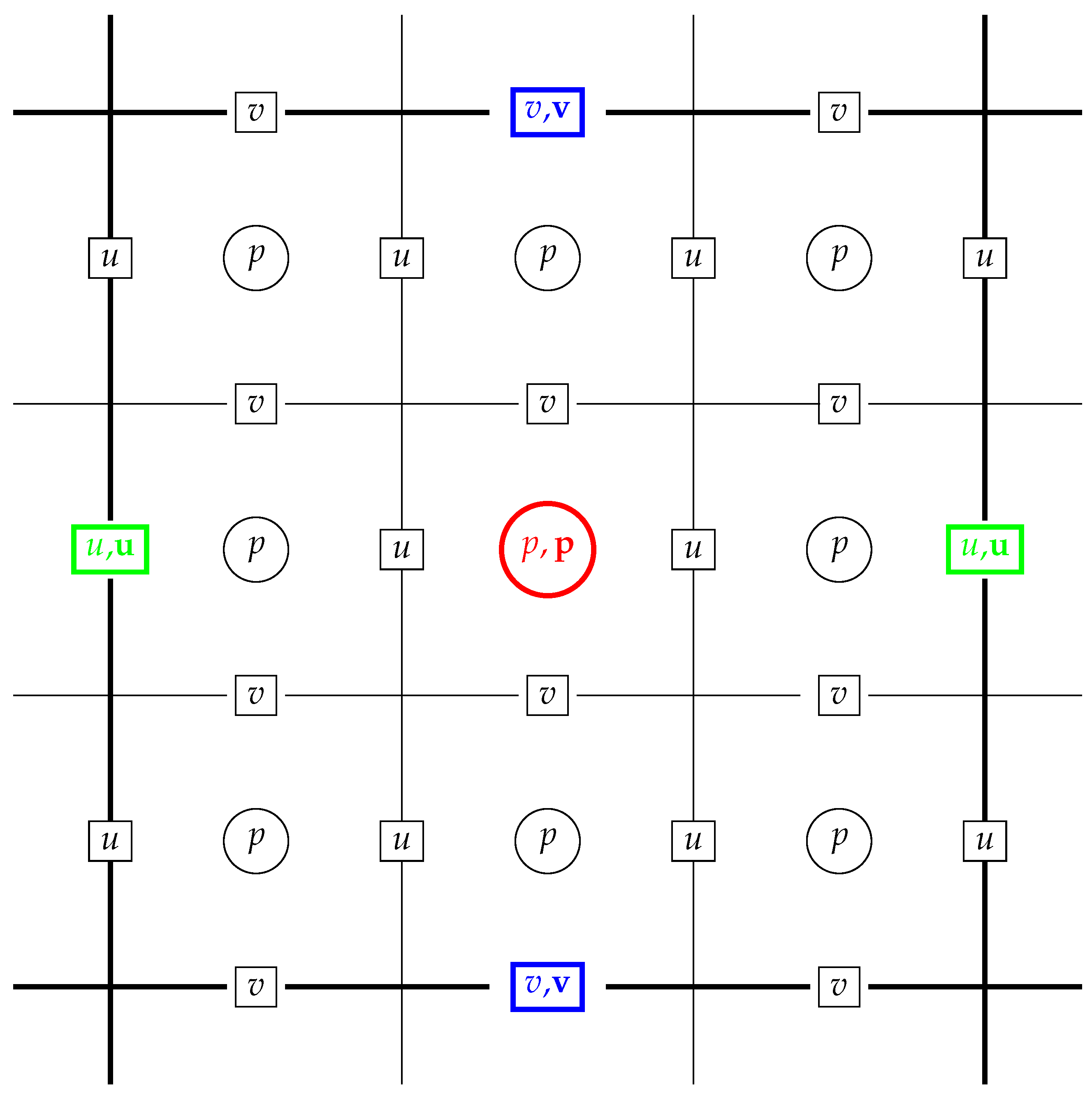
In the following, the discretization of stochastic Stokes equations (state equation) is presented. Note that, on staggered grids, the variables $u,v,p$ are defined on ${\mathsf{\Omega }}_h^{ev},{\mathsf{\Omega }}_h^{eh}$, and ${\mathsf{\Omega }}_h^c$, respectively (see Figure 1). Thus, by finite differences, we have

$$\begin{array}{ccc}\hfill -{\Delta }^h{\mathbf{u}}_j^h+{\partial }_j^h{p}^h& =& {\mathbf{f}}_j^h+\sigma {\dot{\mathbf{W}}}_h^j,\mathrm{at}\mathrm{centers}\mathrm{of}j-\mathrm{faces}\hfill \\ \hfill \sum _{j=1}^2{\partial }_j^h{\mathbf{u}}_j^h& =& 0,\mathrm{at}\mathrm{cell}\mathrm{centers}\hfill \end{array}$$

where ${\Delta }^h$ denotes the discrete Laplace operator, i.e., the five-point approximation. We approximate the first-order partial derivative by (second-order) central differences. For example, to discretize the pressure variable p at the cell center $(h_x/2,h_y/2)$, we have ${\partial }_x^h$ and ${\partial }_y^h$ as follows:

$$\begin{array}{ccc}\hfill {\partial }_x^{h}p(x,y)& =& \frac{u(x+h_x/2,y+h_y/2)-u(x-h_x/2,y+h_y/2)}{h_x},\hfill \\ \hfill {\partial }_y^{h}p(x,y)& =& \frac{u(x+h_x/2,y+h_y/2)-u(x+h_x/2,y-h_y/2)}{h_y}.\hfill \end{array}$$

Note that, for a point near a boundary, ${\Delta }^h{\mathbf{u}}_j^h\left(\mathbf{x}\right)$ may involve an exterior value, and, to find these exterior values, quadratic extrapolation is used (cf. [17,27]).

Next, to have a more insight about the discretization using finite differences on staggered grid, we proceed as follows: set $x_i=(i-1)h$ and $y_j=(j-1)h$. By $p_{i+1/2,j+1/2}$, we mean the discrete counterpart to $p(x_i+h/2,y_j+h/2)$. and we consider the grid indices in lexicographic order. In this way, we come up with the state system given by

$$\begin{array}{ccc}\hfill -{\Delta }_h{u}^h+\frac{p_{i-1/2,j+1/2}-p_{i-3/2,j+1/2}}{h_x}& =& f_{i,j+1/2}+\sigma W_h^1,\mathrm{on}{\mathsf{\Omega }}_h^{ev}\hfill \end{array}$$

(15)

$$\begin{array}{ccc}\hfill -{\Delta }_h{v}^h+\frac{p_{i+1/2,j-1/2}-p_{i+1/2,j-3/2}}{h_y}& =& g_{i+1/2,j}+\sigma W_h^2,\mathrm{on}{\mathsf{\Omega }}_h^{eh}\hfill \end{array}$$

(16)

$$\begin{array}{ccc}\hfill \frac{u_{i+1,j+1/2}-u_{i,j+1/2}}{h_x}+\frac{v_{i+1/2,j+1}-v_{i+1/2,j}}{h_y}& =& 0,\mathrm{on}{\mathsf{\Omega }}_h^c\hfill \end{array}$$

(17)

where (15) and (16) are defined on ${\mathsf{\Omega }}_h^{ev}$ and ${\mathsf{\Omega }}_h^{eh}$, respectively. Moreover, the continuity Equation (17) is defined on ${\mathsf{\Omega }}_h^c$.

The optimality conditions $\alpha f-\lambda =0$ and $\alpha g-\mu =0$ illuminate that, for the adjoint equation, the variables u and $\lambda ,f$ are defined on ${\mathsf{\Omega }}_h^{ev}$ and the variables v, g, and $\mu$ are defined on ${\mathsf{\Omega }}_h^{eh}$. Moreover, in the continuity equation for state (respectively, adjoint), the variable p and q appears on mesh cell centers ${\mathsf{\Omega }}_h^c$. Thus, in this way, we obtain the following discretized adjoint equation:

$$\begin{array}{ccc}\hfill -{\Delta }_h{\lambda }^h+\frac{q_{i-1/2,j+1/2}-q_{i-3/2,j+1/2}}{h_x}& =& {(U-u)}_{i,j+1/2},\mathrm{on}{\mathsf{\Omega }}_h^{ev}\hfill \end{array}$$

(18)

$$\begin{array}{ccc}\hfill -{\Delta }_h{\mu }^h+\frac{q_{i+1/2,j-1/2}-q_{i+1/2,j-3/2}}{h_y}& =& {(V-v)}_{i+1/2,j},\mathrm{on}{\mathsf{\Omega }}_h^{eh}\hfill \end{array}$$

(19)

$$\begin{array}{ccc}\hfill \frac{{\lambda }_{i+1,j+1/2}-{\lambda }_{i,j+1/2}}{h_x}+\frac{{\mu }_{i+1/2,j+1}-{\mu }_{i+1/2,j}}{h_y}& =& 0\mathrm{on}{\mathsf{\Omega }}_h^c.\hfill \end{array}$$

(20)

Here, we remark that, with our approach, a direct coupling among the state, adjoint, and control variables has e been implemented with the help of optimality conditions (on staggered grids) and thus requires no additional computations (interpolation).

Summarizing, the discretize optimality system consists of Equations (15)–(20) with the optimality conditions given by

$$\begin{array}{ccc}\hfill \alpha f_{i,j+1/2}-{\lambda }_{i,j+1/2}& =& 0,\mathrm{on}{\mathsf{\Omega }}_h^{ev}\hfill \\ \hfill \alpha g_{i+1/2,j}-{\mu }_{i+1/2,j}& =& 0,\mathrm{on}{\mathsf{\Omega }}_h^{eh}\hfill \end{array}$$

(21)

with boundary conditions given by

$$\begin{array}{ccc}\hfill u_{i,j+1/2}& =& 0,\hfill \\ \hfill v_{i+1/2,j}& =& 0,\hfill \\ \hfill {\lambda }_{i,j+1/2}& =& 0,\hfill \\ \hfill {\mu }_{i+1/2,j}& =& 0.\hfill \end{array}$$

(22)

4. Multigrid

The multigrid framework to solve the optimality system is presented in this section. In the development of multigrid solver, we face some difficulties due to the coupled nature of the state and adjoint equations on the staggered grid structure.

It is a well known fact that multigrid methods involves discretization grids. For example, we obtain such grids by halving the mesh size starting from the coarsest grid [13,14]. In the context of staggered grid multigrid approach and in our previous works [27,28,31], multigrid schemes for the optimal control problems constrained by Stokes equations and/or PDEs, we note that, by tripling the mesh size, starting from the coarsest staggered grid, gives a nested hierarchy of grid that helps in simplifying the intergrid transfer operators. The details are as follows:

In the following, we define a sequence of grids ${\mathsf{\Omega }}_k$ of mesh size $h_k=h_1/3^{(k-1)}$, $k=1,\cdots ,L$, where $k=L$ is the finest level and $h_1=1/2$ is the mesh sizes of the coarsest grid. We denote the index k to define the functions (operators) on ${\mathsf{\Omega }}_k$. Moreover, with three-factor coarsening, setting a variable $X_{IJ}^{k-1}$ on the coarse grid ${\mathsf{\Omega }}_{k-1}$ has the same location as the variable $X_{ij}^k$ on the fine grid ${\mathsf{\Omega }}_k$. Figure 1 presents an example.

• $u_{I,J+1/2}^{k-1}⟷u_{ij}^k$, for $i=3I-2$, $j=3J-1$.
• $v_{I+1/2,J}^{k-1}⟷v_{ij}^k$, for $i=3I-1$, $j=3J-2$.
• $p_{I+1/2,J+1/2}^{k-1}⟷p_{ij}^k$, for $i=3I-1$, $j=3J-1$.

4.1. Smoothing Scheme

In this section, we present the smoothing scheme to relax the state (respectively, adjoint) momentum equations and the state (respectively, adjoint) continuity equation by a distributive relaxation [17]. A line search is used to update the control variable.

We denote $(u^h,v^h,p^h,{\lambda }^h,{\mu }^h,q^h,f^h,g^h)$ as the discrete counterpart to the numerical approximation to our optimization problem. Then, we update this approximation step by step iteratively, which is explained as follows. First, we update the control variable by the gradient update step (line search) with gradient of the so-called reduced cost functional, i.e, ${\nabla }_f\widehat{J}(f_h,g_h)=\alpha f_h-{\lambda }_h$, ${\nabla }_g\widehat{J}(f_h,g_h)=\alpha g_h-{\mu }_h$ as follows

$$\begin{array}{ccc}\hfill f_h& \leftarrow & f_h-t{\nabla }_f\widehat{J},\hfill \\ \hfill g_h& \leftarrow & g_h-t{\nabla }_g\widehat{J},\hfill \end{array}$$

(23)

where the step size for the control update is $t\in (0,1]$.

Then, we consider the sate equation and let $(u^h,v^h,p^h)$ be its approximation. We smooth the residuals of the state system (15)–(16) by the classical Gauss–Seidel (pointwise) relaxation. Next, we use distributive relaxation (cf. [17,27]) to relax the variable $p^h$ corresponding to the continuity Equation (17).

Next, we relax the adjoint equation as done for the discretized state equation. That is, the residuals of the adjoint system (18)–(19) are smoothed by the classical pointwise Gauss–Seidel scheme at all the interior points. Moreover, the (adjoint) continuity Equation (20) is relaxed by a distributive relaxation (cf. [27,28]).

In the following, we discuss the intergrid transfer operators for the proposed multigrid framework. We use bilinear interpolation to interpolate the (state and adjoint) variables and residual functions. For example, for the variable u, consider the space ${\mathcal{U}}_k$ of $u^k:{\mathsf{\Omega }}_k^{ev}\to \mathbb{R}$, $k=1,\dots ,L$. Between the two grids, the fine grid ${\mathsf{\Omega }}_k$ and the coarser grid ${\mathsf{\Omega }}_{k-1}$, we define a prolongation operator, i.e., $I_{k-1}^k:{\mathcal{U}}_{k-1}\to {\mathcal{U}}_k$. Here, we assume that (for the discretization) this prolongation operator is consistent with the bilinear finite elements on each rectangular partition.

We use a straight injection operator as our restriction operator in the proposed multigrid solver. Note that, in the three-factor coarsening strategy, the location or position of the state (respectively, adjoint) variables on the coarse-grid and the fine-grid are the same (see Figure 1). Therefore, we use straight injection operator $I_k^{k-1}:{\mathcal{U}}_k\to {\mathcal{U}}_{k-1}$ to transfer the residuals (solution) functions from fine to coarse grids. We also remark here that one can use the other operators such as half weighting or full weighting but this may increase the computations without any gain (efficiency). We employ straight injection because it is the advantage of the three-factor coarsening strategy on staggered grid and therefore a natural choice in this case.

4.2. Algorithms

Here, we present the algorithms for a full multigrid method (FMG) (see [14]). Since we know that the FMG method improves the computational complexity of a full approximation scheme (FAS), we use the full multigrid method to solve the discretized optimality system and hence the optimization problem.

To develop a multigrid algorithm, we consider the optimality system (15)–(22) corresponding to the stochastic Stokes control problem, at the discretization level k. Let the unknown variable be $X_k=(u_k,v_k,p_k,{\lambda }_k,{\mu }_k,q_k,f_k,g_k)$. Then, we can write the optimality system given by

$$A_k\left(X_k\right)=F_k.$$

(24)

Let $X_k^{\left(l\right)}=S_k(X_k^{(l-1)},F_k)$ be the smoothing result as given in Section 4.1. Then, starting with $X_k^{\left(0\right)}$, we obtain the approximate solution, e.g. ${\tilde{X}}_k=X_k^{\left(m_1\right)}$, after $m_1$-times (iterations).

For completeness, we present the full approximation scheme (FAS) in Algorithm 1:

Algorithm 1: FAS$(m_1,m_2)$ for solving $A_k\left(X_k\right)=F_k$.

If $k=1$ solve $A_k\left(X_k\right)=F_k$ exactly. Pre-smoothing steps on the fine grid: $X_k^{\left(l\right)}=S_k(X_k^{(l-1)},F_k)$, $l=1,\cdots ,m_1$; Computation of the residual: $r_k=F_k-A_k\left(X_k^{\left(m_1\right)}\right)$; Restriction of the residual: $r_{k-1}=I_k^{k-1}{r}_k$; Set $X_{k-1}=I_k^{k-1}{X}_k^{\left(m_1\right)}$; Set $F_{k-1}=r_{k-1}+A_{k-1}\left(X_{k-1}\right)$ Call m times MG$(m_1,m_2)$ to solve $A_{k-1}\left(X_{k-1}\right)=F_{k-1}$; Coarse-grid correction: $X_k^{(m_1+1)}=X_k^{\left(m_1\right)}+I_{k-1}^k(X_{k-1}-I_k^{k-1}{X}_k^{\left(m_1\right)})$; Post-smoothing steps on the fine grid: $X_k^{\left(l\right)}=S_k(X_k^{(l-1)},F_k)$, $l=m_1+2,\cdots ,m_1+m_2+1$;

In this algorithm, we can perform m two-grid iterations at each working level. For $m=1$, we have a V-cycle, and, for $m=2$, we have a W-cycle [14].

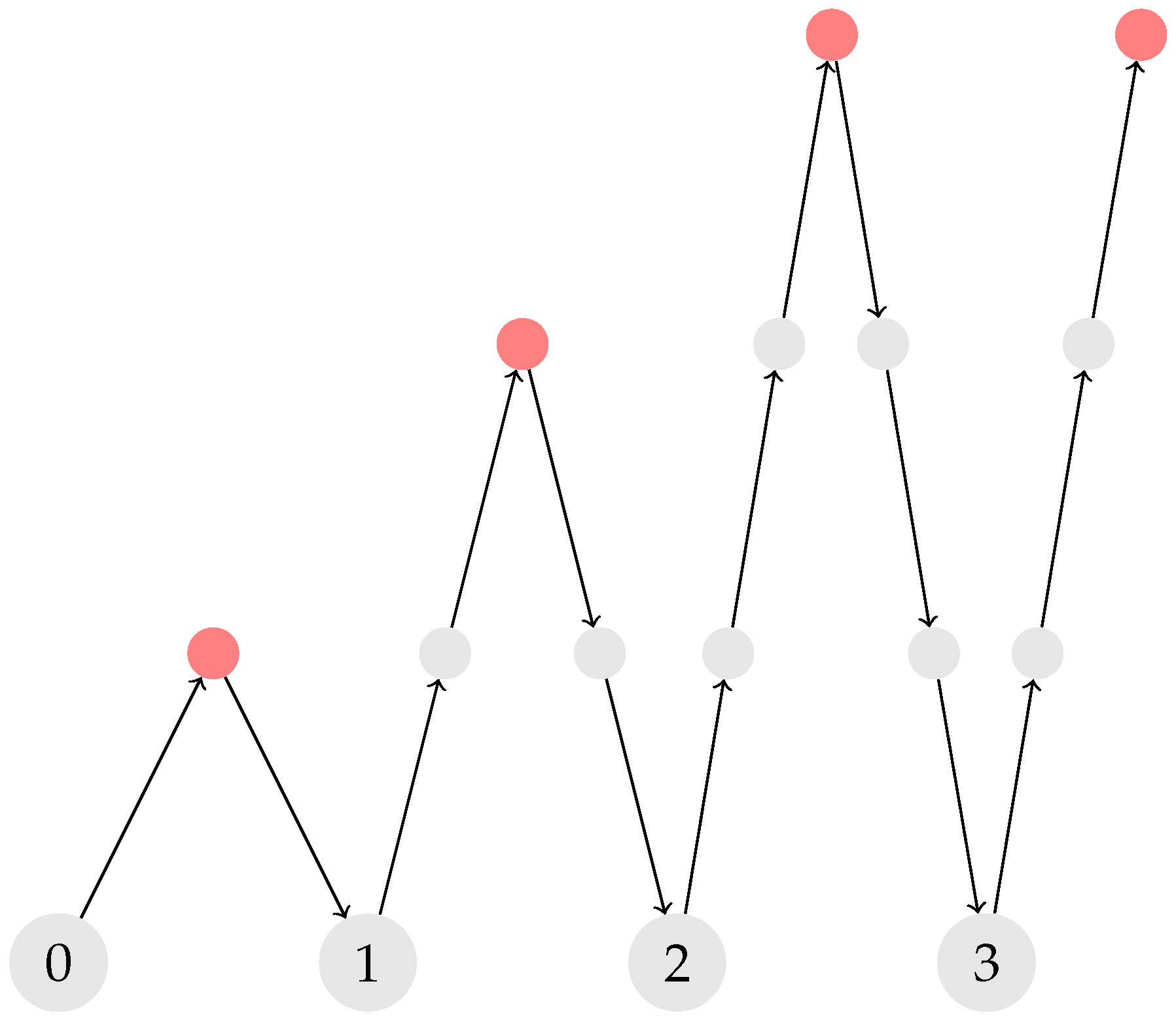
As is known, with a better initial guess, we can use fewer iterations [14]. Moreover, the FAS is implemented as a subroutine that improves the nonlinearity issues (if required in the problem). Therefore, a full multigrid (FMG) method (see Figure 2) is employed in this article and in Algorithm 2 form it is given as follows:

Algorithm 2: FMG for solving $A_L\left(X_L\right)=F_L$.

For $l=K<L$, set initial approximation $u_l$. If $l<L$, then interpolate to the next finer working level: ${\tilde{X}}_{l+1}=I_l^{l+1}{X}_l$; Apply FAS to solve $A_{l+1}\left(X_{l+1}\right)=F_{l+1}$, starting with ${\tilde{X}}_{l+1}$; Set $l:=l+1$; If $l<L$ go to step 2; else stop.

5. Numerical Experiments

We considered the following optimization problem constrained by the stochastic Stokes equations to show the numerical results:

$$\begin{array}{ccc}\hfill \mathrm{Min}J(\mathbf{u},\mathbf{f})& =& \frac{1}{2}{\int }_{\mathsf{\Omega }}{|\mathbf{u}-\mathbf{U}|}^{2}dx+\frac{\alpha }{2}{\int }_{\mathsf{\Omega }}{\left|\mathbf{f}\right|}^{2}dx,\hfill \\ \hfill \text{subject} \text{to}\\ \hfill -\nu ▵\mathbf{u}+\nabla p& =& \mathbf{f}+\sigma \dot{\mathbf{W}},\mathrm{in}\mathsf{\Omega }\hfill \\ \hfill -\nabla ·\mathbf{u}& =& 0,\mathrm{in}\mathsf{\Omega }\hfill \\ \hfill \mathbf{u}& =& 0,\mathrm{on}\Gamma .\hfill \end{array}$$

(25)

We set $\sigma =0.1$ and $\nu =1$ and solved the control problem on various meshes and regularization parameter $\alpha >0$, in the numerical experiments. We took a rectangular domain $\mathsf{\Omega }={[0,1]}^2$ with uniform mesh size and used MATLAB(2020b) to develop a code for solving the control problem numerically, on a laptop i7 with 1.3 GHz, 16 GB RAM.

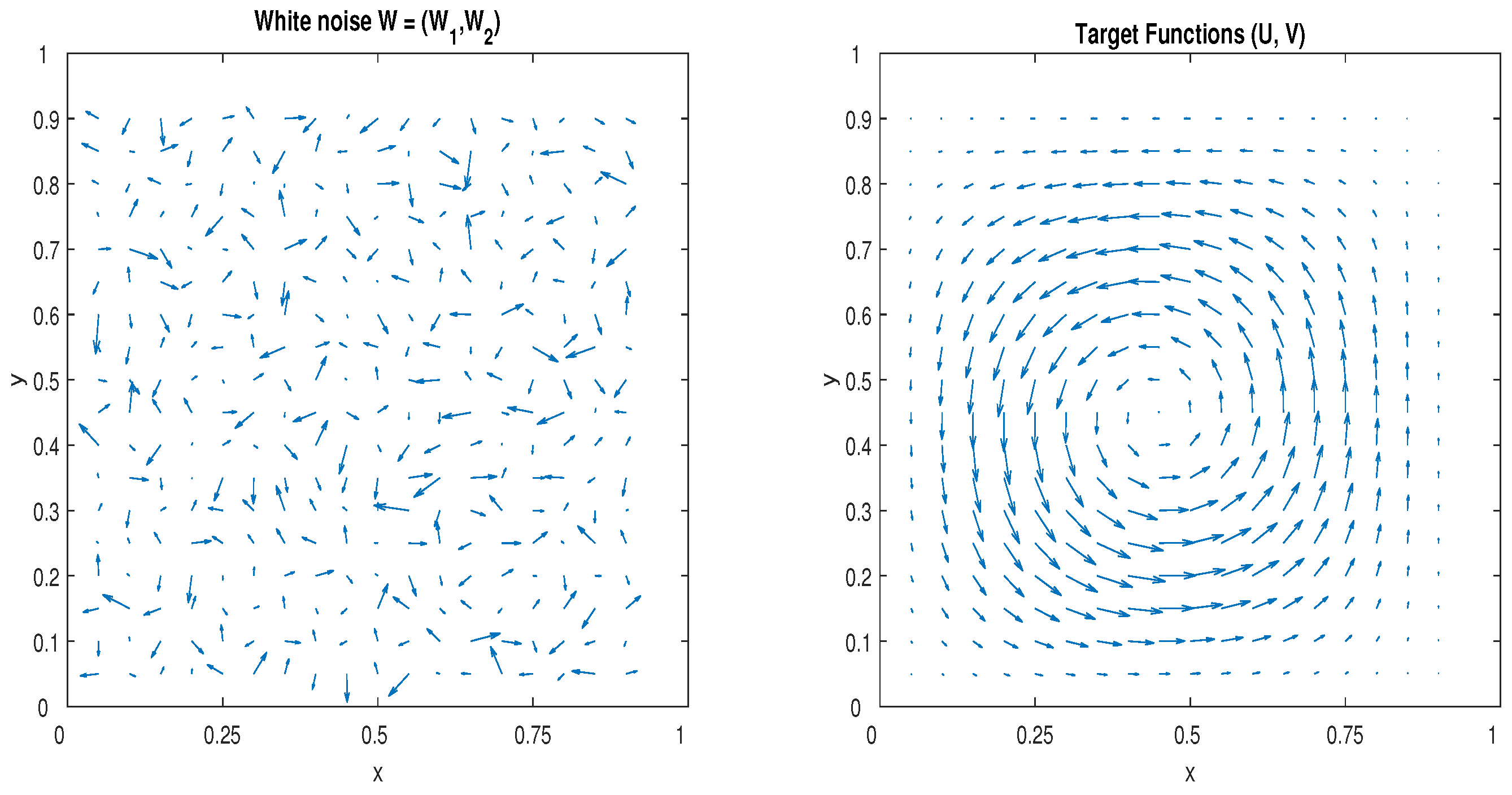
For our control problem, we do not need an exact solution. Therefore, we took the desired velocity [8] $\mathbf{U}=\left(U\right(x,y),V(x,y\left)\right)$ given by

$$U(x,y)=10\frac{d}{dy}\psi \left(x\right)\psi \left(y\right)\mathrm{and}V(x,y)=-10\frac{d}{dx}\psi \left(x\right)\psi \left(y\right)$$

where

$$\psi \left(z\right)={(1-z)}^2(1-cos\left(0.8\pi z\right)).$$

In Figure 3, a vector field of random velocities with the white noise is presented. Moreover, we depict the target velocity in vector form in Figure 3.

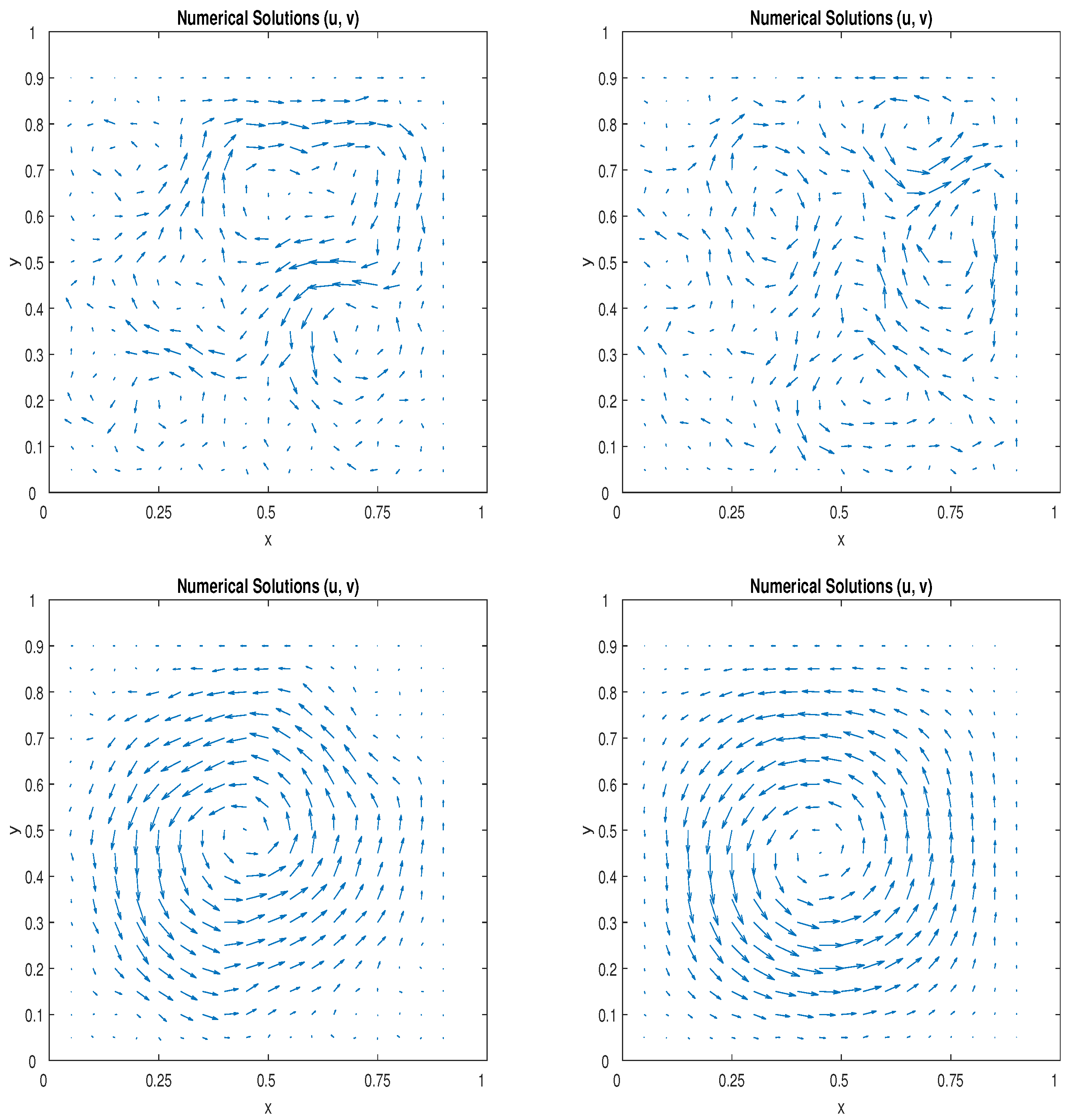
For the numerical solution of this control problem, we used the proposed FMG Algorithm 2. A W-cycle with $4-pre$ and $4-post$ smoothing steps was employed, that is, we took $m_1=m_2=4$ in Algorithm 2). One can also use the $V-cycles$, but we did not find any improvement during our investigation. Furthermore, we chose $t=1$ as the step length in the control update step. For the stopping criteria, we used the discrete $L^2$-norm of all the variables $(u_h,v_h,p_h,{\lambda }_h,{\mu }_h,q_h)$, that is, we stopped the iterations when

$$\max \left\{\parallel r_{jh}{\parallel }_{L^2\left({\mathsf{\Omega }}_h\right)}\right\}<{10}^{-6}.$$

As expected, we have a better tracking for the desired (target) velocity field as $\alpha \to 0$ (see

Table 1. Tracking errors on ${18}^2$ mesh.

$\mathit{\alpha }$	$\parallel {\mathbf{u}}^{\mathit{h}}-{\mathbf{U}}^{\mathit{h}}{\parallel }_{{\mathit{L}}^2\left({\mathbf{\Omega }}_{\mathit{h}}\right)}$	$\widehat{\mathit{J}}\left({\mathbf{f}}^{\mathit{h}}\right)$
${10}^{-1}$	4.3742 × 10−1	1.9203 × 10−1
${10}^{-2}$	4.2916 × 10−1	1.9080 × 10−1
${10}^{-3}$	3.0231 × 10−1	1.2330 × 10−1
${10}^{-4}$	9.7101 × 10${}^{-2}$	3.8977 × 10${}^{-2}$
${10}^{-5}$	2.3830 × 10${}^{-2}$	6.0480 × 10${}^{-3}$

). This fact is illustrated in Figure 4, that is, as $\alpha \to 0$ the optimal velocities match the desired vector filed (see

Table 2. Iteration counts and CPU time for stochastic Stokes control problem.

${\mathit{N}}_{\mathit{x}}\times {\mathit{N}}_{\mathit{y}}$	$6^2$	${18}^2$	${54}^2$
$\alpha ={10}^{-1}$	14	10	09
CPU(sec)	(0.43)	(0.63)	(1.09)
$\alpha ={10}^{-2}$	146	100	80
CPU(sec)	(0.90)	(1.87)	(4.99)
$\alpha ={10}^{-3}$	1383	999	741
CPU(sec)	(4.04)	(12.88)	(35.13)
$\alpha ={10}^{-4}$	8566	8606	6740
CPU(sec)	(20.86)	(73.80)	(522.20)

, Figure 3).

6. Conclusions

A multigrid scheme to solve the stochastic Stokes control problem with additive white noise is presented. On staggered grids, a three-factor coarsening strategy is employed, which results in nested hierarchy of staggered-grids. To solve the discretized optimality system with finite differences and noise, a line search strategy to update the control and a distributive relaxation scheme to relax the state (respectively, adjoint) variables is employed. Moreover, to discretize the additive white noise, we simply consider the Gaussian noise at the discretized level in our numerical investigation. Numerical results illuminate the efficiency and the ability of the proposed multigrid solver to track the desired target (velocity vector field) while the Stokes equations were driven by force term with additive white noise.

In comparison to the recent work [8] on the numerical solution of stochastic Stokes control problems with additive white noise, we note that our multigrid solver provides better iteration counts due to three-factor coarsening strategy, i.e., fewer levels, less computational cost, and less CPU time.

The proposed multigrid method can be extended to the three-dimensional case, i.e., stochastic Stokes control problem with noise in 3D staggered-grid multigrid framework. Moreover, one can investigate the Navier–Stokes control problems with noise, which is a natural extension of our present work.

References

- Lions, J.L. Optimal Control of Systems Governed by Partial Differential Equations; Springer: Berlin, Germany, 1971. [Google Scholar]
- Tröltzsch, F. Optimal Control of Partial Differential Equations: Theory, Methods and Applications; AMS: Providence, RI, USA, 2010. [Google Scholar]
- Babuska, I.; Chatzipantelidis, P. On solving elliptic stochastic partial differential equations. Comput. Methods Appl. Mech. Eng. 2002, 191, 4093–4122. [Google Scholar] [CrossRef]
- Babuska, I.; Tempone, R.; Zouraris, G.E. Galerkin finite element approximations of stochastic elliptic partial differential equations. SIAM J. Numer. Anal. 2004, 42, 800–825. [Google Scholar] [CrossRef]
- Babuska, I.; Tempone, R.; Zouraris, G.E. Solving elliptic boundary value problems with uncertain coefficients by the finite element method: The stochastic formulation. Comput. Methods Appl. Mech. Eng. 2005, 194, 1251–1294. [Google Scholar] [CrossRef]
- Cao, Y.; Chen, Z.; Gunzburger, M.D. Error analysis of finite element approximations of the stochastic Stokes equations. Adv. Comput. Math. 2010, 33, 215–230. [Google Scholar] [CrossRef]
- Chen, P.; Quarteroni, A.; Rozza, G. Multilevel and weighted reduced basis method for stochastic optimal control problems constrained by stokes equations. Numer. Math. 2016, 133, 67–102. [Google Scholar] [CrossRef]
- Choi, Y.; Lee, H.-C. Error analysis of finite element approximations of the optimal control problem for stochastic Stokes equations with additive white noise. Appl. Numer. Math. 2018, 133, 144–160. [Google Scholar] [CrossRef]
- Gunzburger, M.; Lee, H.-C.; Lee, J. Error estimates of stochastic optimal neumann boundary control problems. SIAM J. Numer. Anal. 2011, 49, 1532–1552. [Google Scholar] [CrossRef]
- Hou, L.; Lee, J.; Manouzi, H. Finite element approximations of stochastic optimal control problems constrained by stochastic elliptic PDEs. J. Math. Anal. Appl. 2011, 384, 87–103. [Google Scholar] [CrossRef] [Green Version]
- Lee, H.-C.; Gunzburger, M. Comparison of approaches for random PDEoptimization problems based on different matching functionals. Comput. Math. Appl. 2017, 73, 1657–1672. [Google Scholar] [CrossRef]
- Brandt, A. Multi-level adaptive solutions to boundary-value problems. Math. Comp. 1977, 31, 333–390. [Google Scholar] [CrossRef]
- Hackbusch, W. Multi-Grid Methods and Applications; Springer: New York, NY, USA, 1985. [Google Scholar]
- Trottenberg, U.; Oosterlee, C.; Schüller, A. Multigrid; Academic Press: London, UK, 2001. [Google Scholar]
- Benzi, M.; Golub, G.H.; Liesen, J. Numerical solution of saddle point problems. Acta Numer. 2005, 14, 1–137. [Google Scholar] [CrossRef] [Green Version]
- Zulehner, W. Nonstandard norms and robust estimates for saddle point problems. SIAM J. Matrix Anal. Appl. 2011, 32, 536–560. [Google Scholar] [CrossRef] [Green Version]
- Brandt, A.; Dinar, N. Multigrid Solutions to Elliptic Flow Problems, Numerical Methods for Partial Differential Equations; Parter, S., Ed.; Academic Press: New York, NY, USA; London, UK, 1979; pp. 53–147. [Google Scholar]
- Brandt, A.; Yavneh, I. On Multigrid Solution of High-Reynolds Incompressible Entering Flows. J. Comput. Phys. 1992, 101, 151–164. [Google Scholar] [CrossRef] [Green Version]
- Girault, V.; Raviart, P.-A. Finite Element Methods for Navier–Stokes Equations: Theory and Algorithms; Springer Series in Computational Mathematics; Springer: Berlin, Germany, 1986; Volume 5. [Google Scholar]
- Kellogg, R.B.; Osborn, J.E. A regularity result for the Stokes problem in a convex polygon. J. Funct. Anal. 1976, 21, 397–431. [Google Scholar] [CrossRef] [Green Version]
- Oosterlee, C.W.; Gaspar, F.J. Multigrid methods for the Stokes system. Comput. Sci. Eng. 2006, 8, 34–43. [Google Scholar] [CrossRef]
- Takacs, S. A robust all-at-once multigrid method for the Stokes control problem. Numer. Math. 2015, 130, 517–540. [Google Scholar] [CrossRef] [Green Version]
- Wang, W.; Chen, L. Multigrid Methods for the Stokes Equations using Distributive Gauss-Seidel Relaxations based on the Least Squares Commutator. J. Sci. Comput. 2013, 56, 409–431. [Google Scholar] [CrossRef]
- Wittum, G. Multi-grid methods for Stokes and Navier-Stokes equations. Numer. Math. 1989, 54, 543–563. [Google Scholar] [CrossRef]
- Borzì, A.; Schulz, V. Multigrid methods for PDE optimization. SIAM Rev. 2009, 51, 361–395. [Google Scholar] [CrossRef]
- Rees, T.; Wathen, A.J. Preconditioning Iterative Methods for the Optimal Control of the Stokes Equations. SIAM J. Sci. Comput. 2011, 33, 2903–2926. [Google Scholar] [CrossRef]
- Butt, M.M. A multigrid solver for Stokes control problems. Int. J. Comput. Math. 2017, 94, 2297–2314. [Google Scholar] [CrossRef]
- Butt, M.M.; Yuan, Y. A full multigrid method for distributed control problems constrained by Stokes equations. Numer. Math. Theory Methods Appl. 2017, 10, 639–655. [Google Scholar] [CrossRef]
- Noack, B.R.; Morzynski, M.; Tadmor, G. Reduced-Order Modelling for Flow Control, 1st ed.; Springer: Wien, Austria, 2011. [Google Scholar]
- Ito, K.; Kunisch, K. Lagrange Multiplier Approach to Variational Problems and Applications; SIAM: Philadelphia, PA, USA, 2008. [Google Scholar]
- Butt, M.M.; Borzì, A. Formulation and multigrid solution of Cauchy-Riemann optimal control problems. Comput. Vis. Sci. 2011, 14, 79–90. [Google Scholar] [CrossRef]
Figure 1.
Three-factor coarsening on staggered grids.
Figure 2.
Full multigrid (FMG) method on three levels. The red circles denotes the initial guess after prolongation ↗ (interpolation) and ↘ shows the restriction.
Figure 3.
The realization of the white noise (left) and the target velocity field (right) on mesh ().
Figure 4.
Optimal solution (velocity vector field): (top left) ; (top right) ; (bottom left) ; and (bottom right) on mesh.