Random Sampling Many-Dimensional Sets Arising in Control ^†

Abstract

Various Monte Carlo techniques for random point generation over sets of interest are widely used in many areas of computational mathematics, optimization, data processing, etc. Whereas for regularly shaped sets such sampling is immediate to arrange, for nontrivial, implicitly specified domains these techniques are not easy to implement. We consider the so-called Hit-and-Run algorithm, a representative of the class of Markov chain Monte Carlo methods, which became popular in recent years. To perform random sampling over a set, this method requires only the knowledge of the intersection of a line through a point inside the set with the boundary of this set. This component of the Hit-and-Run procedure, known as boundary oracle, has to be performed quickly when applied to economy point representation of many-dimensional sets within the randomized approach to data mining, image reconstruction, control, optimization, etc. In this paper, we consider several vector and matrix sets typically encountered in control and specified by linear matrix inequalities. Closed-form solutions are proposed for finding the respective points of intersection, leading to efficient boundary oracles; they are generalized to robust formulations where the system matrices contain norm-bounded uncertainty.

1. Introduction

One of the first issues in data mining and pattern recognition is an economy representation of implicitly specified massive data arrays with the subsequent extraction of specific features and classification [1,2,3]. Every element of the data set can be associated with a vector of which the components are the numerical values of certain properties of the phenomenon of interest under one or another operating condition. As a rule, a complete description of the data is not available due to high dimensions and cardinality, and the very absence of an explicit “generating” mechanism. Instead, a representative enough sample from the data set may be considered, leading to a point representation of the respective continuum domain, and the desired characteristics can then be measured just at these sample points.

There exist many ways to organize such samples. The most obvious one is to arrange a deterministic rectangular grid over the respective many-dimensional domain. However, this approach suffers several drawbacks. First, for high dimensions, the density of the grid needed for a reasonable representation of the set is very large; second, it can be efficiently implemented only for box-shaped sets; finally, sets that differ from rectangles may be embedded into larger boxes, however, the so-called rejection rate (the amount of “idle” grid points lying outside the domain of interest) may grow very quickly with the growth of dimension. A more efficient technique relates to the generation of quasi-random points in the feasible domain; they are also referred to as $L{P}_{\tau }$ sequences introduced in [4]; however, this mechanism heavily exploits the box shape of the set. For the discussion of these questions, see [5] and the references therein.

Since recently, a purely randomized approach to the solution of various problems in the above-mentioned fields became very popular [6]. The overall idea is to embed a deterministic formulation of the problem into a stochastic setup and to obtain an approximate solution, which is “close” to that of the original problem with certain probability. Often, such a reformulation considerably diminishes computational efforts; moreover, the associated probabilities can be efficiently estimated. This is particularly important for many-dimensional problems involving massive data arrays and containing various uncertainties and inaccuracies.

As compared to deterministic techniques, straightforward random sampling can be applied to a much wider class of sets; still, its application is limited to “regular” sets in a sense, for example, such as those bounded in some vector or matrix norm [6]. However, it often happens that the only information about the set is available in the form of the so-called boundary oracle, which is formulated as follows. Given a point inside the set and an arbitrary line through it, the oracle returns the intersection points of this line and the boundary of the set. The term “boundary oracle” introduced presumably in [7] originates in the optimization theory, where various assumptions on the available information about the function under minimization and the constraint set lead to estimates of complexity of the corresponding optimization methods [8,9]. For instance, search methods assume just the knowledge of the function value at any point; in first-order methods, the derivative is also available, i.e., we possess the gradient oracle; in second-order methods, on top of that we also have a Hessian oracle. The same goes for the constraint set, for which various assumptions (such as membership oracle, separation oracle) are adopted [9].

One of the efficient sampling procedures that are based on the availability of boundary oracles is the Hit-and-Run (HR) algorithm, which was proposed in [10] with the primary goal to facilitate numerical calculation of multi-dimensional integrals over convex domains. It became popular after the publication of [11], and later, various modifications and ramifications of this algorithm were proposed; for example, see [12,13]. In particular, a promising Markov chain sampler, the billiard walk exploits “reflections” of a moving particle from the boundary of a convex set. It was deeply analyzed in [14] and showed itself rather efficient; however, it requires not only the availability of a boundary oracle but also the information about the curvature of the boundary, and is more time-consuming in implementation.

The basic HR procedure is very simple in implementation and requires little information about the problem. It was proved to have a polynomial mixing time; i.e., the number of iterations required to “approximately” reach the desired theoretical distribution grows polynomially in the dimension [12]. In applications, it possesses quite fast practical convergence for so-called isotropic sets. It also can be generalized to deal with non-convex sets and to produce limiting distributions that differ from the uniform one. At the same time, the algorithm is not free of drawbacks. First, the proved theoretical convergence is very slow. Also, the method tends to get stuck at the corners of “thin” non-isotropic sets; on the other hand, there exist modifications of the HR algorithm, which are capable of escaping the corners [15].

Overall, the Hit-and-Run is widely considered to be one of the preferred practical and theoretical tools for uniform sampling inside large-dimensional convex bodies; for example, see [14,16,17]. Moreover, in [17], a comparison tool was proposed to quantify the performance of several commonly used Markov chain sampling techniques, and it turned out that the basic HR procedure outperforms other approaches and is less intensive computationally.

Those interested in the history of the HR algorithm are referred to [10,11,12]; later developments can be found in [18] and also in [19,20], where a promising modification using barrier functions was proposed; of the most recent papers we mention [17,21,22].

The HR algorithm has found applications in random sampling inside various sets (non-convex and not connected as well), approximate computation of the volume of convex sets [23] and, most efficiently, in the probabilistic approach to numerical optimization. For the latter, see, for example, [24,25], where the authors proposed new versions of the cutting plane scheme for use in efficient methods of optimization. Namely, the HR points were generated with the aim of approximating the center of gravity of the support set of the optimized function. Other applications include random walks in graph spaces [26], machine learning [16,27], etc. In particular, for a specific determinantal point process problem, a version of the HR sampler based on the zonotopic structure of the problem was proposed in [16]. This approach, though being faster than the conventional HR, requires solving additional linear programs and is not easy to implement.

However, in spite of a wide range of applications of the Hit-and-Run sampler, to the best of our knowledge, almost no research was devoted to its use in control. Perhaps the only paper in this direction is [28], where this method was applied to the design of stabilizing controllers in the simplest form.

In this paper we do not deal with applications of the HR to specific control problems; this is the subject for future research. Nor do we analyze the convergence and optimization of the performance of the HR algorithm. Instead, we limit ourselves to the considerations related to its BO component, and propose several numerical schemes for the implementation of this component.

In principle, instead of having a BO, the availability of a weaker membership oracle might be assumed, and a straightforward line search can then be used. However, this search has to be performed many times, so that it is important to provide a “closed-form” solution to this operation in order to improve the performance of the algorithm. By closed-form solution we also mean various numerical procedures such as finding the roots of a polynomial or the eigenvalues of a matrix, solving semidefinite programs (SDPs) of moderate size and the like. These operations are indeed very fast and numerically efficient in the standard Matlab implementation.

In this paper, we propose efficient computations of several BOs for various vector and matrix sets defined by linear matrix inequalities (LMIs).

The sets that we analyze in the paper appear in control problems in a natural way, and we consider sets specified by LMIs in the canonical form, the classical matrix Lyapunov inequality, and algebraic matrix Riccati inequalities. We also pay attention to various robust versions of these inequalities, where the matrix coefficients contain additive uncertainty.

We focus on the sets defined by LMIs because of the generality and flexibility of this technique and it is wide spread in systems theory; see the classical book [29] and the recent survey paper [30]. Overall, LMI-sets describe a wast variety of convex sets. Notably, because of convexity, only two intersection points are to be found.

One of the few works in this research direction is the conference paper [31], where first attempts were made to the implementation of such boundary oracles. Since then, possible applications of the HR algorithm became broader, and some of them motivated us to get back to this subject and consider it in a different context. For instance, one of the novel applications of this technique might be processing huge data arrays obtained from ultrasound computed tomography in medical diagnostics; for example, such as in [32]. This may lead to fast image reconstruction algorithms and improve the quality of the image.

In the current paper several major changes are performed as compared to [31]. The introduction section is completely re-written to better substantiate the importance of the research; for the same purpose, the order of the exposition and the overall wording is changed, the bibliography list is considerably extended to account for the new available developments, some proofs are added and some of them are corrected and made more transparent, several mathematical inaccuracies in the exposition are also corrected, many new notations are introduced to facilitate the understanding of the material, and typos are removed.

The notation used in the paper is very standard. Namely, ${\mathbb{R}}^n$ and ${\mathbb{R}}^{k\times m}$ denote the space of real column vectors of length n and real $k\times m$ matrices; ${}^{\top }$ is the transposition sign; ⊕ and ⊗ stand for the Kronecker sum and Kronecker product of two matrices; the signs $\prec ,\succ ,\preccurlyeq ,\succcurlyeq$ denote the negative (positive) definiteness (semidefiniteness) of a matrix; $\parallel ·\parallel$ is the Euclidean vector norm or the spectral or the Frobenius matrix norm (this will be clear from the context); $W^{1/2}$ is the matrix square root of the positive-definite matrix W.

We use the following acronyms:

• BO—Boundary Oracle;
• HR—Hit-and-Run;
• LMI—Linear Matrix inequality;
• LQR—Linear Quadratic Regulation;
• SDP—SemiDefinite Programming.

2. Background and an Illustration

2.1. The Hit-and-Run Procedure

We briefly formulate the main components of the HR procedure as applied to convex sets and uniform distributions.

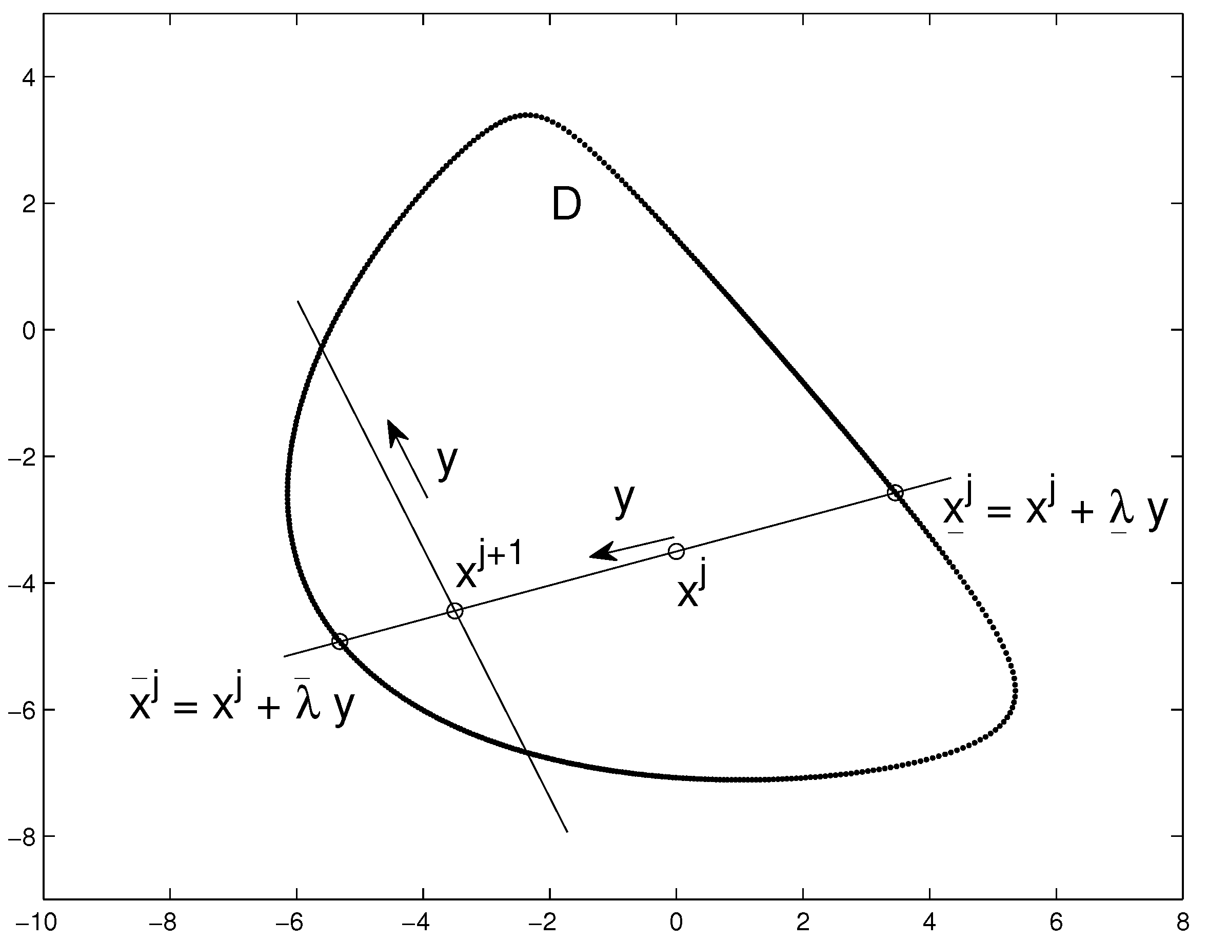
Denote by $x^0\in {\mathbb{R}}^n$ an initial point in the interior of a closed convex bounded domain $\mathcal{D}\subset {\mathbb{R}}^n$, and let $x^j$ denote the point generated at the jth step of the procedure. The next point is generated as follows. First, a random unit-length vector $y\in {\mathbb{R}}^n$ is generated uniformly on the sphere in ${\mathbb{R}}^n$ and the line $x^j+\lambda y$ through this point in the direction y is considered. Denote by ${\underline{x}}^j$ and ${\overline{x}}^j$ the points of intersection of this line and the boundary of $\mathcal{D}$; they are assumed to be obtained with the use of BO. Then the next point $x^{j+1}$ is generated uniformly randomly on the segment $[{\underline{x}}^j,{\overline{x}}^j]$, a new random direction is generated, etc. The scheme of the HR algorithm is presented in Figure 1 for $n=2$.

In the HR-related literature it is shown that, under mild conditions on the set $\mathcal{D}$ and the choice of initial $x^0$, the resulting sequence of random points tend to the uniform distribution over $\mathcal{D}$ as the number of points grow.

It is interesting to note that the HR method and particularly, its BO component can be used not only for generating points inside sets, but also for approximate point description of the boundary of implicitly specified sets. This description is obtained at no extra cost by simply memorizing the “side-product” endpoints ${\underline{x}}^j$ and ${\overline{x}}^j$. We note that there exist specialized methods that generate points exactly on the boundary of the sets of interest [33].

2.2. Illustration: Static Output Feedback Stabilization

Let us consider a linear time invariant system in the state-space description

$$\begin{array}{ccc}\hfill \dot{x}& =& Ax+Bu,\hfill \\ \hfill y& =& Cx.\hfill \end{array}$$

(1)

Here the system matrices $A\in {\mathbb{R}}^{n\times n}$, $B\in {\mathbb{R}}^{n\times m}$, $C\in {\mathbb{R}}^{k\times m}$ are fixed and known. Assume that there exists a static output control $u=Ky$ that makes the closed-loop matrix $A+BKC$ Hurwitz stable, and let the set $\mathcal{D}\subset {\mathbb{R}}^{k\times m}$ of all such stabilizing gain matrices K be bounded. A typical control problem is to optimize certain “engineering” performance indices over the set of these matrix gains, such as overshoot, oscillation, damping time.

First, it is well known that the very existence of a stabilizing output feedback is hard to establish [34], not talking about optimizing such a control. Second, the engineering performance indices mentioned above are not easy to formalize and optimize even in a much simpler situation where state feedback is considered.

As an alternative to the existing techniques we can instead arrange random sampling over the domain $\mathcal{D}$, compute the value of the performance index for each sample, and pick the best one. This approach to optimal controller design suggests the availability of a representative enough sample set in $\mathcal{D}$, and it can be obtained by using the HR-algorithm. In its simplest form this approach was considered in [35,36], where only low-order controllers were considered and the domain $\mathcal{D}$ was two-dimensional. No random sampling was used, but the authors suggested to pick a point in $\mathcal{D}$ with a mouse on the computer screen and compute the respective performance index. Such a “manual” semi-heuristic approach, being very simple, often leads to controllers that outperform those obtained by the methods available in the literature.

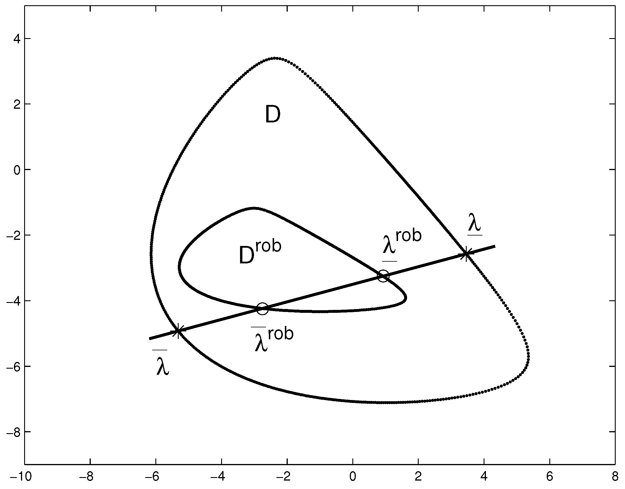
To arrange the HR algorithm in the general many-dimensional setting, assume that we possess a feasible $K\in \mathcal{D}$, denote by $L\in {\mathbb{R}}^{k\times m}$ a matrix direction, take $K+\lambda L$ instead of K, and consider the $\lambda$-dependent $n\times n$ matrix $A+B(K+\lambda L)C$, where $\lambda \in \mathbb{R}$. Then the goal of the BO is to find the minimum $\underline{\lambda }$ and maximum $\overline{\lambda }$ values of $\lambda \in \mathbb{R}$ that guarantee the stability of $A+B(K+\lambda L)C$ over the whole segment $[\underline{\lambda },\overline{\lambda }]$.

To further simplify notation, denote $A_0: =A+BKC$ and $A_1: =BLC$; then we have $A+B(K+\lambda L)C=A_0+\lambda A_1$, where $A_0$ is stable. Hence, the boundary oracle reduces to finding the so-called unidirectional stability segment of maximum length [37].

For the clarity of the overall exposition, we present the corresponding result.

Lemma 1

([37]). Let $A_0,A_1\in {\mathbb{R}}^{n\times n}$, and let $A_0$ be Hurwitz stable. The minimal and the maximal values of the parameter $\lambda \in \mathbb{R}$ that guarantee the stability of $A_0+\lambda A_1$ are defined by

$$\underline{\lambda }=\left\{\begin{array}{cc}{\displaystyle \frac{1}{\underset{{\lambda }_i<0}{min}{\lambda }_i}},& \hfill \\ & \\ -\infty ,& ifall{\lambda }_i>0;\hfill \end{array}\right.$$

(2)

$$\overline{\lambda }=\left\{\begin{array}{cc}{\displaystyle \frac{1}{\underset{{\lambda }_i>0}{max}{\lambda }_i},}& \hfill \\ & \\ +\infty ,& ifall{\lambda }_i<0,\hfill \end{array}\right.$$

(3)

where ${\lambda }_i$ are real eigenvalues of the matrix $-{(A_0\oplus A_0)}^{-1}(A_1\oplus A_1)$, and $A\oplus A$ denotes the Kronecker sum.

We recall that the Kronecker sum of the two square matrices A and B is defined as $A\oplus B=A\otimes I_a+I_b\otimes B$, where $I_a,I_b$ are identity matrices of appropriate dimensions and ⊗ stands for the Kronecker product of matrices.

Back to our problem, we see that the matrix segment $[K+\underline{\lambda }L;K+\overline{\lambda }L]$ obtained with the use of the lemma above belongs to the set $\mathcal{D}$ of output stabilizing gain matrices. Therefore, the next matrix (i.e., the next HR point) is then generated randomly on this segment.

Unfortunately, in Lemma 1 one has to compute eigenvalues of $n^2\times n^2$ matrices, which makes computations slow for high dimensions. For instance, already for $n=25$, the computations would take about a second on a standard laptop, which is considered rather slow, keeping in mind multiple executions of this procedure as required in the HR-algorithm. On the other hand, (i) typically, problems arising in control are of lower dimensions, and (ii) the availability of boundary oracle can be relaxed to the assumption of having a membership oracle, so that a boundary oracle can always be constructed by means of a linear search. However, for a wide range of problems, a boundary oracle can be easily formulated in closed form, and below we present particular boundary oracles for matrix sets specified by linear matrix inequalities.

3. LMI Sets in Canonical Form

We turn to formation of boundary oracles related to sets defined by linear matrix inequalities and consider LMIs in the canonical form.

3.1. The Uncertainty-Free Setup

Introduce the following matrix-valued function of a vector variable:

$$F_0+\sum _{i=1}^n{x}_i{F}_i\doteq F\left(x\right),$$

(4)

where $x={(x_1,\cdots ,x_n)}^{\top }\in {\mathbb{R}}^n$ is the variable and $F_i=F_i^{\top }\in {\mathbb{R}}^{m\times m}$, $i=0,\cdots ,n$, are fixed matrix coefficients.

Consider the convex domain defined as

$$\mathcal{D}=\{x\in {\mathbb{R}}^n:F\left(x\right)\preccurlyeq 0\},$$

(5)

where the sign ≼ denotes the negative semidefiniteness of a matrix, and we assume that $\mathcal{D}$ as nonempty.

Let $x,y\in {\mathbb{R}}^n$ be, respectively, a point in the interior of $\mathcal{D}$ and a direction. To formulate a boundary oracle for this domain, we need to compute the minimal and the maximal values $\underline{\lambda },\overline{\lambda }$ of the scalar parameter $\lambda \in \mathbb{R}$ that guarantee the sign-definiteness of $F(x+\lambda y)$ over the interval $[\underline{\lambda },\overline{\lambda }]$. We have

$$F(x+\lambda y)=F_0+\sum _{i=1}^n\left(x_{+}\lambda y_i\right)F_i\doteq A_0+\lambda A_1.$$

where we denoted $A_0:=F\left(x\right)$ and $A_1:={\sum }_{i=1}^n{y}_i{F}_i$.

It is seen that $A_0\prec 0$ and $A_1=A_1^{\top }$; hence, similarly to the above, the goal is to compute the minimum and the maximum values of $\lambda \in \mathbb{R}$ that guarantee the sign-definiteness of the affine matrix function $A_0+\lambda A_1$. The lemma below is a slight modification of the result in [7] it shows that this can be done by computing the generalized eigenvalues of the matrix pair $(A_0,-A_1)$.

Lemma 2.

Let $A_0\prec 0$ and $A_1=A_1^{\top }$, then the critical values of the scalar λ that guarantee negative semidefiniteness of the matrix function $A_0+\lambda A_1$ are obtained as:

$$\underline{\lambda }=\left\{\begin{array}{cc}\underset{{\lambda }_i<0}{max}{\lambda }_i,& \hfill \\ & \\ -\infty ,& ifall{\lambda }_i>0;\hfill \end{array}\right.$$

(6)

$$\overline{\lambda }=\left\{\begin{array}{cc}\underset{{\lambda }_i>0}{min}{\lambda }_i,& \hfill \\ & \\ +\infty ,& ifall{\lambda }_i<0,\hfill \end{array}\right.$$

(7)

where ${\lambda }_i$ are the generalized eigenvalues of the matrix pair $(A_0,-A_1)$; i.e., $A_0{e}_i=-{\lambda }_i{A}_1{e}_i$.

Proof. 

The proof is nearly trivial: The critical value of $\lambda$ that makes the matrix $A_0+\lambda A_1$ sign indefinite is also responsible for the loss of nonsingularity; by definition, this means that there exists a nonzero $e\in {\mathbb{R}}^m$ such that $(A_0+\lambda A_1)e=0$.    □

This result of the lemma above applies to symmetric matrices; i.e., it is a special case of Lemma 1, since a symmetric matrix is stable if and only if it is negative definite.

As far as the initial point $x^0\in \mathrm{int}\mathcal{D}$ is considered, it can be found as a solution $\{\widehat{x},\widehat{\eta }\}$ of the following SDP:

$$min\eta \text{subject}\mathrm{to}F\left(x\right)\preccurlyeq \eta I.$$

(8)

If $\widehat{\eta }>0$, the set $\mathcal{D}$ (5) is empty; otherwise we adopt $x^0=\widehat{x}$.

3.2. A Robust Formulation

We now consider the situation where the matrix coefficients $F_i$ in (4) contain uncertainties. Specifically, they have the form $F_i+{\Delta }_i$, where ${\Delta }_i\in {\mathbb{R}}^{m\times m}$ are bounded in the spectral norm $\parallel {\Delta }_i\parallel \le {\epsilon }_i$, $i=0,\cdots ,n$, and mutually independent, and ${\epsilon }_i\ge 0$ are given levels of uncertainty. To retain the symmetric structure of the matrices $(F_i+{\Delta }_i)$, the ${\Delta }_i$’s are also assumed to be symmetric. We call such uncertainties admissible.

As a result, we obtain the uncertain linear matrix-valued function

$$F(x,\Delta )=(F_0+{\Delta }_0)+\sum _{i=1}^n{x}_i(F_i+{\Delta }_i)$$

of the vector variable $x\in {\mathbb{R}}^n$ and the respective (convex) robustly feasible domain

$${\mathcal{D}}^{\mathrm{rob}}=\{x\in {\mathbb{R}}^n:F(x,\Delta )\preccurlyeq 0\mathrm{for}\mathrm{all}\mathrm{admissible}{\Delta }_i\}.$$

Likewise the uncertainty-free setup, having an $x\in \mathrm{int}{\mathcal{D}}^{\mathrm{rob}}$ and a directional vector $y\in {\mathbb{R}}^n$, we aim to compute the minimal ${\underline{\lambda }}^{\mathrm{rob}}$ and maximal ${\overline{\lambda }}^{\mathrm{rob}}$ values of the parameter $\lambda$ that guarantee that the uncertain LMI $F(x+\lambda y,\Delta )\preccurlyeq 0$ holds for all admissible uncertainties ${\Delta }_i$ over the segment $[{\underline{\lambda }}^{\mathrm{rob}},{\overline{\lambda }}^{\mathrm{rob}}]$. This procedure will be referred to as robust boundary oracle.

The construction of the feasible and the associated robustly feasible domains is depicted in Figure 2 for $x\in {\mathbb{R}}^2$, the same symmetric matrices $F_0,F_1,F_2\in {\mathbb{R}}^{3\times 3}$ that were used in the example of Figure 1, and certain numerical values of ${\epsilon }_i$.

Here, $\underline{\lambda }$ and $\overline{\lambda }$ denote the critical values of the parameter $\lambda$ obtained via formulae (6) and (7) for the corresponding uncertainty-free formulation in Lemma 2.

From the lemma below, Reference [7] presents the robust BO for the uncertain LMI $F(x,\Delta )\preccurlyeq 0$; it amounts to solving certain nonlinear equations in one scalar variable.

Lemma 3.

Let $x\in \mathrm{int}{\mathcal{D}}^{\mathrm{rob}}$ and $y\in {\mathbb{R}}^n$ be given. Consider the two functions in the variable $\lambda \in \mathbb{R}$:

$$\varphi \left(\lambda \right)=∥{\left(F_0+\sum _{i=1}^n(x_i+\lambda y_i)F_i\right)}^{-1}∥,$$

$${\displaystyle \epsilon \left(\lambda \right)=\frac{1}{{\epsilon }_0+{\displaystyle \sum _{i=1}^n}|x_i+\lambda y_i|{\epsilon }_i}.}$$

The critical values ${\underline{\lambda }}^{\mathrm{rob}}$ and ${\overline{\lambda }}^{\mathrm{rob}}$ of the parameter λ, which guarantee that the matrix $F(x+\lambda y,\Delta )$ is negative definite for all admissible Δ, are found as the two solutions of the equation $\varphi \left(\lambda \right)=\epsilon \left(\lambda \right)$ on the segment $[\underline{\lambda },\overline{\lambda }]$ obtained in (6) and (7).

Clearly, the robust BO is more laborious than its uncertainty-free analog; indeed, not only a specific nonlinear equation is to be solved numerically, but the nonrobust bounds $\underline{\lambda }$ and $\overline{\lambda }$ are to be computed as well.

The proof of Lemma 3 uses the same basic reasonings: The loss of robust sign-definiteness of the matrix function $F(x+\lambda y,\Delta )$ coincides with the loss of nonsingularity for some admissible ${\Delta }_i$s. The proof heavily exploits the independence of the ${\Delta }_i$s and uses the symmetric analog of Theorem 3 in [38] on the radius of matrix nonsingularity.

In Figure 3, the plots of the functions $\varphi \left(\lambda \right)$ and $\epsilon \left(\lambda \right)$ are depicted for an uncertain LMI with $x\in {\mathbb{R}}^4$, and the desired segments for $\lambda$ are shown.

4. Quadratic Stabilization

From this section onward we switch our attention from “abstract” LMIs in vector variables to those encountered in control problems; namely, to specific LMIs in matrix variables.

4.1. The Lyapynov Boundary Oracle

First of all we consider the Lyapunov inequality

$$AX+X{A}^{\top }+G\prec 0,$$

(9)

where $G=G^{\top }$ and A are given and $X=X^{\top }$ is the $n\times n$ matrix variable.

This inequality naturally appears in the design of stabilizing state feedback controllers for continuous-time systems. Specifically, consider the system $\dot{x}=Ax+Bu$ (1) with controllable pair $(A,B)$; then the gain matrix K for the stabilizing control $u=Kx$ may be found as $K=-B^{\top }{X}^{-1}$, where $X\succ 0$ is a solution of the LMI (9) with $G=-2B{B}^{\top }$, and $V\left(x\right)=x^{\top }{X}^{-1}x$ is a quadratic Lyapunov function for the closed-loop system [29].

Therefore, the convex closed set of matrices

$$\mathcal{D}=\{X\in {\mathbb{R}}^{n\times n}:AX+X{A}^{\top }+G\preccurlyeq 0,X\succcurlyeq 0\}$$

(10)

specified by the LMI (9) is of obvious interest in control design, and we formulate its boundary oracle.

Such an oracle is seen to be computed with the use of Lemma 2. Given an $X\in \mathrm{int}\mathcal{D}$ and a matrix direction $Y=Y^{\top }$, we obtain

$$A(X+\lambda Y)+(X+\lambda Y)A^{\top }+G\preccurlyeq 0.$$

Denoting $A_0:=AX+X{A}^{\top }+G$ and $A_1:=AY+Y{A}^{\top }$ and keeping in mind that $A_0\prec 0$ and $A_1=A_1^{\top }$, we find ourselves in the conditions of Lemma 2, which gives us the interval ${\Lambda }_A$ of sign-definiteness of the $\lambda$-dependent function $A_0+\lambda A_1$. Since the matrix $X+\lambda Y$ is to be positive definite (as the matrix of a Lyapunov function), we again use Lemma 2 to calculate the corresponding range ${\Lambda }_X$ of $\lambda$ retaining the sign-definiteness of $X+\lambda Y$. Then adopt $\Lambda ={\Lambda }_A\cap {\Lambda }_X$ as the desired maximal interval of $\lambda$ for which the matrix $X+\lambda Y$ belongs to $\mathcal{D}$ (10).

4.2. A Robust Formulation

The Lyapunov BO of the previous subsection can be generalized to the situation where the matrix A in (9) contains uncertainty. We consider the model of structured uncertainty, which often appears in control applications:

$$A(\Delta )=A+M\Delta N.$$

(11)

Here the matrix perturbation $\Delta \in {\mathbb{R}}^{p\times q}$ is only known to be bounded in some norm $\parallel \Delta \parallel \le 1$, and the matrices $M\in {\mathbb{R}}^{n\times p}$, $N\in {\mathbb{R}}^{q\times n}$ are given.

In such a setup, the uncertain Lyapunov inequality

$$A(\Delta )X+X{A}^{\top }(\Delta )+G\preccurlyeq 0$$

(12)

is used for the construction of a common quadratic Lyapunov function with matrix X for the uncertain system and yields robustly stabilizing controllers.

This gives rise to the robust Lyapunov set

$${\mathcal{D}}^{\mathrm{rob}}=\left\{X\succcurlyeq 0:\text{inequality}\left(12\right)\mathrm{holds}\mathrm{for}\mathrm{all}\parallel \Delta \parallel \le 1\right\},$$

(13)

and the goal is to devise a boundary oracles for it.

The main technical trick for operating with uncertainty (11) is the so-called Petersen lemma proposed in [39]; it provides necessary and sufficient conditions for an uncertain matrix to be sign-definite.

Lemma 4.

Assume that $R=R^{\top }\in {\mathbb{R}}^{n\times n}$, $P\in {\mathbb{R}}^{n\times p}$, $Q\in {\mathbb{R}}^{q\times n}$. Then, for the inequality

$$R+P\Delta Q+{(P\Delta Q)}^{\top }\preccurlyeq 0$$

(14)

to hold for all $\Delta \in {\mathbb{R}}^{p\times q}$, $\parallel \Delta \parallel \le 1$, it is necessary and sufficient that there exist $\epsilon >0$ such that

$$R+\epsilon P{P}^{\top }+\frac{1}{\epsilon }{Q}^{\top }Q\preccurlyeq 0.$$

(15)

We stress that, with the lemma above, checking the robust sign-definiteness of a continuum matrix family reduces to a convex problem in one scalar variable. To see this, using the Schur complement, represent inequality (15) in the equivalent form

$$\left(\begin{array}{cc}R+\epsilon P{P}^{\top }& Q^{\top }\\ & \\ Q& -\epsilon I\end{array}\right)\preccurlyeq 0,$$

(16)

which is an LMI in the scalar variable $\epsilon$.

Moreover, with this machinery, the maximal admissible span for the uncertainty $\Delta$ can be found:

$${\gamma }_{max}=sup\{\gamma :\mathrm{inequality}\left(14\right)\mathrm{holds}\mathrm{for}\mathrm{all}\parallel \Delta \parallel \le \gamma \}.$$

(17)

It is sometimes called the radius of robust sign-definiteness of the uncertain matrix $R+P\Delta Q+{(P\Delta Q)}^{\top }$; computing this quantity reduces to the solution of a semidefinite program in two scalar variables and a “scaled” LMI constraint of the form (16), see [40].

With the Petersen lemma in mind, we are ready to formulate the boundary oracle for the set (13); it will be referred to as the robust Lyapunov BO.

Theorem 1.

Assume that $X\in {\mathcal{D}}^{\mathrm{rob}}$ (11)–(13) and $Y=Y^{\top }\in {\mathbb{R}}^{n\times n}$ are given. Denote ${\Lambda }_A=[\underline{\lambda },\overline{\lambda }]$, where $\underline{\lambda }$ and $\overline{\lambda }$ are found as the solutions of the two semidefinite programs:

$$min/max\lambda subjectto$$

$$\left(\begin{array}{cc}AX+X{A}^{\top }+G+\lambda (AY+Y{A}^{\top })+\epsilon M{M}^{\top }& X{N}^{\top }+\lambda Y{N}^{\top }\\ & \\ NX+\lambda NY& -\epsilon I\end{array}\right)\preccurlyeq 0,X+\lambda Y\succcurlyeq 0$$

in the scalar variables $\lambda ,\epsilon$.

The maximum interval of $\lambda \in \mathbb{R}$ that guarantees $X+\lambda Y\in {\mathcal{D}}^{\mathrm{rob}}$ is given by $\Lambda ={\Lambda }_A\cap {\Lambda }_X$, where ${\Lambda }_X\subset \mathbb{R}$ denotes the maximal interval of sign-definiteness of the pencil $X+\lambda Y$.

Proof. 

Having a feasible $X\in {\mathcal{D}}^{\mathrm{rob}}$ defined by (11)–(13), and a matrix direction Y, we are aimed at finding the minimum and the maximum values of $\lambda$ for which the inequality

$${(A+M\Delta N)}^{\top }(X+\lambda Y)+(X+\lambda Y)(A+M\Delta N)+G\preccurlyeq 0$$

(18)

is satisfied for all $\parallel \Delta \parallel \le 1$.

To simplify notation, let us denote

$$R\left(\lambda \right)=AX+X{A}^{\top }+G+\lambda (AY+Y{A}^{\top })$$

and

$$P=M;Q\left(\lambda \right)=N(X+\lambda Y);$$

then (18) takes the compact form

$$R\left(\lambda \right)+P\Delta Q\left(\lambda \right)+{\left(P\Delta Q\left(\lambda \right)\right)}^{\top }\preccurlyeq 0.$$

By Petersen lemma, this inequality holds for all admissible $\parallel \Delta \parallel \le 1$ and for some $\lambda$ if and only if there exist $\epsilon >0$ such that

$$\left(\begin{array}{cc}R\left(\lambda \right)+\epsilon P{P}^{\top }& Q^{\top }\left(\lambda \right)\\ & \\ Q\left(\lambda \right)& -\epsilon I\end{array}\right)\preccurlyeq 0.$$

Since the functions $R\left(\lambda \right)$ and $Q\left(\lambda \right)$ are affine in $\lambda$, the last inequality is seen to be an LMI in the two scalar variables $\lambda$ and $\epsilon$. Therefore, finding the critical values of $\lambda$ reduces to the minimization and maximization of the variable $\lambda$ subject to the LMI constraint above. Finally, the maximum interval of the sign-definiteness of the matrix $X+\lambda Y$ is found using Lemma 2.    □

We make two comments at this point.

First, an initial $X\in \mathrm{int}{\mathcal{D}}^{\mathrm{rob}}$ can be obtained from the solution $\{\widehat{X},\widehat{\eta },\widehat{\epsilon }\}$ of the following SDP in the matrix variable X and two scalar variables $\eta ,\epsilon$:

$$min\eta \mathrm{subject}\mathrm{to}$$

$$\left(\begin{array}{cc}AX+X{A}^{\top }+G+\epsilon M{M}^{\top }& X{N}^{\top }\\ & \\ NX& -\epsilon I\end{array}\right)\preccurlyeq \eta I,X\succcurlyeq 0.$$

(19)

In complete analogy with (8), if $\widehat{\eta }<0$, adopt $X=\widehat{X}$; otherwise the set ${\mathcal{D}}^{\mathrm{rob}}$ (13) is empty.

This observation leads to the second comment. If the LMIs (19) are infeasible, we decrease the level of uncertainty and re-solve the SDP to test the nonemptiness of ${\mathcal{D}}^{\mathrm{rob}}$. On the other hand, by solving a similar semidefinite program, the maximal allowed level

$${\gamma }^{\mathrm{rob}}=max\{\gamma :\exists X\succcurlyeq 0:\mathrm{inequality}\left(12\right)\mathrm{holds}\mathrm{for}\mathrm{all}\parallel \Delta \parallel \le \gamma \},$$

the radius of robust quadratic stabilizability can be calculated in advance; cf. (17) and see [30,40] for the details.

5. Optimal Control

Assume now that, on top of stabilizing system (1) by means of linear control $u=Kx$, we want to optimize a certain performance index.

In one of the classical optimal control problems, the linear quadratic regulation (LQR) problem, the quadratic cost functional has the form

$$J\left(K\right)={\int }_0^{\infty }(x^{\top }{W}_{x}x+u^{\top }{W}_{u}u)\mathrm{d}t,$$

where $W_x\succ 0$ and $W_u\succ 0$ are weight matrices. The minimization of this cost leads to the algebraic Riccati equation

$$X{W}_{x}X+AX+X{A}^{\top }-B{W}_u^{-1}{B}^{\top }=0$$

in the matrix variable X; under certain conditions on $A,B$ its unique positive-definite solution defines the optimal gain $K=-W_u^{-1}{B}^{\top }{X}^{-1}$.

5.1. The Riccati Boundary Oracle

In a slightly more general formulation consider the set

$$\mathcal{D}=\{X\in {\mathbb{R}}^{n\times n}:X{W}_{x}X+AX+X{A}^{\top }-G\preccurlyeq 0,X\succ 0\},$$

(20)

where $G\succcurlyeq 0$ is a given real $n\times n$ matrix. This set accumulates all possible solutions $X\succ 0$ of the algebraic Riccati inequality, and the boundary oracle for this set is formulated in much the same way as in Section 4.1, with Lemma 2 as the main tool.

Indeed, let us first take the Schur complement and represent the quadratic inequality in the LMI form:

$$\left(\begin{array}{cc}AX+X{A}^{\top }-G& X{W}_x^{1/2}\\ & \\ W_x^{1/2}X& I\end{array}\right)\preccurlyeq 0.$$

Next, considering $X+\lambda Y$ instead of X, we arrive at

$$A_0+\lambda A_1\preccurlyeq 0,$$

with

$$A_0=\left(\begin{array}{cc}AX+X{A}^{\top }-G& X{W}_x^{1/2}\\ & \\ W_x^{1/2}X& I\end{array}\right)\preccurlyeq 0$$

and

$$A_1=\left(\begin{array}{cc}AY+Y{A}^{\top }& Y{W}_x^{1/2}\\ & \\ W_x^{1/2}Y& I\end{array}\right)=A_1^{\top }.$$

Hence we are again in the conditions of Lemma 2, which gives us the associated segment ${\Lambda }_A$.

Next, accounting for the sign definiteness of the matrix $X+\lambda Y$ and using Lemma 2 once again, we obtain the corresponding feasible segment ${\Lambda }_X$ and adopt ${\Lambda }_A\cap {\Lambda }_X$ as the final answer.

Overall, the computation of the boundary oracle for the set defined by the quadratic inequality reduces to the Lyapunov BO described in Section 4.1; the only essential difference is that now the size of the constraint matrices is twice as large as before.

5.2. A Robust Formulation

Let now the matrix A be subjected to the uncertainty of the same structured form (11). The corresponding robust counterpart of the LQR problem can be formulated and solved in several ways; for example, see [41]. However, following the logic of the current paper we consider the set

$${\mathcal{D}}^{\mathrm{rob}}=\{X\in {\mathbb{R}}^{n\times n}:X{W}_{x}X+A(\Delta )X+X{A}^{\top }(\Delta )-G\preccurlyeq 0,X\succ 0\}$$

(21)

defined by the uncertain Riccati inequality and propose a boundary oracle for it.

From the exposition of the two previous subsections it is seen that the robust version of the Riccati boundary oracle can be formulated by exploiting the Schur complement (to transform quadratic inequalities into linear ones) and Petersen lemma (to handle the uncertainty). We omit the obvious and not quite insightful derivations and formulate the result in the theorem below.

Theorem 2.

Let $X\in \mathrm{int}{\mathcal{D}}^{\mathrm{rob}}$ (21), (11) and let $Y=Y^{\top }\in {\mathbb{R}}^{n\times n}$. The maximal and the minimal values of λ, which guarantee that the matrix segment $X+\lambda Y$ belongs to the set ${\mathcal{D}}^{\mathrm{rob}}$ (21) are obtained from the solutions of the two semidefinite programs

$$min/max\lambda subjectto$$

$$\left(\begin{array}{cc}{A}_1\left(\epsilon \right)+\lambda A_2& \lambda Z\\ & \\ \lambda Z^{\top }& -I\end{array}\right)\preccurlyeq 0,X+\lambda Y\succcurlyeq 0,$$

where

$$A_1\left(\epsilon \right)=\left(\begin{array}{cc}X{W}_{x}X+AX+X{A}^{\top }-G+\epsilon M{M}^{\top }& X{N}^{\top }\\ & \\ NX& -\epsilon I\end{array}\right);$$

$$A_2=\left(\begin{array}{cc}X{W}_{x}Y+Y{W}_{x}X+AY+Y{A}^{\top }& Y{N}^{\top }\\ & \\ NY& 0\end{array}\right);$$

$$Z=\left(\begin{array}{c}Y{W}_x^{1/2}\\ 0\end{array}\right),$$

and the optimization is performed in the two scalar variables λ and ε.

6. Implementation Issues

We briefly discuss some technical implementation issues and report on the processor time required for the computation of the boundary oracles proposed above.

First, to generate a vector uniformly distributed on the surface of the unit ball in ${\mathbb{R}}^n$, we use the Matlab routine randn to obtain a random vector y with the standard Gaussian distribution and then normalize it to obtain $y=y/\parallel y\parallel$, which is distributed uniformly on the unit sphere. As far as the generation of matrix directions Y in Section 4 and Section 5 is considered, we generate them randomly uniformly on the surface of the unit ball in the Frobenius norm (i.e., on the surface of the ball in ${\mathbb{R}}^{n^2}$) with the subsequent symmetrization.

The main tool for computing the Lyapunov and Riccati BOs, Lemma 2 requires finding generalized eigenvalues of a pair of matrices, and it can be efficiently applied to matrices of rather high dimensions.

The robust boundary oracles in Section 4.2 and Section 5.2 require solving semidefinite programs in two scalar variables with LMI constraints having dimension $2n\times 2n$ (Theorem 1) or $4n\times 4n$ (Theorem 2). To solve these problems, we used the Matlab-compatible software cvx [42].

The following illustrative experiment was performed. We generated randomly $N=1000$ samples of the data required in Lemma 2 and Theorems 1 and 2. For each of these samples, we measured the execution time for the four boundary oracles proposed in the paper, and averaged over N samples. The results obtained on a standard laptop are presented in

Table 1. Execution time (milliseconds) of the four boundary oracles for various dimensions n.

Oracle/Dim	n = 5	n = 10	n = 15	n = 20	n = 30	n = 50
Lyapunov	0.0156	0.0374	0.0883	0.1249	0.3030	0.7279
Riccati	0.0383	0.1241	0.3041	0.4831	1.0686	3.4392
robust Lyapunov	16.0069	22.3414	29.0850	38.2422	62.3214	217.0089
robust Riccati	25.1414	41.5722	67.4951	139.0988	332.3392	1385.8729

.

From the first two rows of the table we see that nonrobust oracles are indeed very fast, since they exploit just the eigenvalue computation, and this operation is “perfectly” implemented in various available toolboxes. Instead, robust boundary oracles are based on solving a specific optimization problem, which is more time-consuming. The last row of the table clearly shows that up to $n=30$, the robust Riccati oracle is fast enough, whereas for $n=50$ the required execution time is approximately one and a half second, which may be considered slow. Note however, that in the latter case, the matrices in the LMI constraints are of quite large size $200\times 200$.

In the experiment, we considered “full” matrices and used the standard freeware cvx for solving semidefinite programs. To speed up the computations in higher dimensions, one may exploit a sparse structure of the system matrices, which is typically the case for control problems, or try to use alternative optimization methods and software. On the other hand, practical control problems have lower dimensions, usually not exceeding $n=15$; see [43], a popular collection of control-related test problems. In other words, in practice, all the proposed BOs seem to be fast enough to be used in sampling the respective sets.

Another observation is that the execution time grows nonlinearly with increase of problem dimension n. This is because the coefficient matrices in the respective LMIs contain $n^2$ elements and because of a specific representation of the LMI constraints in the internal language of cvx solvers. It is also seen that, for a given n, the execution time of the robust Riccati oracle is not exactly the same as that of the robust Lyapunov oracle for the doubled dimension (recall the relative sizes of the respective LMI constraints). This is because the structure of these constraints in the robust Riccati oracle is slightly more complicated.

7. Concluding Remarks and Directions for Future Research

In this paper, we focused on boundary oracles, one of the key components of Hit-and-Run, a popular approach to random generation of points inside bounded sets. We proposed simple computational schemes that implement boundary oracles for several typical control-related matrix sets defined by linear matrix inequalities. At the nucleus of these oracles is the computation of the generalized eigenvalues of a pair of matrices or solving low-dimensional semidefinite programs in scalar variables. These operations are fast as implemented in the Matlab environment, which makes the proposed BOs efficient for use in various random walk methods.

Future research will be targeted at the implementation of boundary oracles for broader classes of sets (e.g., the sets of Schur stable polynomials, positive polynomials, uncertain affine matrix families), which account for the presence of exogenous unknown-but-bounded disturbances, and speeding up the numerical implementation of the HR procedure in these specific problems for higher dimensions. We also note that the results in Section 4 and Section 5 can be easily extended to discrete-time systems by using the discrete-time Lyapunov and Riccati inequalities.

Of the most interest is the application of the machinery presented here to problems of practical interest, in particular, to the design of stabilizing controllers subject to several engineering specifications as mentioned at the beginning of Section 2.2.

References

1. Aggarwal, C.C. Data Mining: The Textbook; Springer: Cham, Switzerland, 2015. [Google Scholar]
2. Bruni, R.; Bianchi, G. Effective classification using a small training set based on discretization and statistical analysis. IEEE Trans. Knowl. Data Eng. 2015, 9, 2349–2361. [Google Scholar] [CrossRef]
3. Blum, A.; Hopcroft, J.; Kannan, R. Foundations of Data Science. Available online: https://www.cs.cornell.edu/jeh/book.pdf (accessed on 8 March 2021).
4. Sobol, I.M. On the distribution of points in a cube and the approximate evaluation of integrals. USSR Comput. Math. Math. Phys. 1967, 4, 86–112. [Google Scholar] [CrossRef]
5. Polyak, B.; Shcherbakov, P. Why does Monte Carlo fail to work properly in high-dimensional optimization problems? J. Optim. Theory Appl. 2017, 2, 612–627. [Google Scholar] [CrossRef] [Green Version]
6. Tempo, R.; Calafiore, G.; Dabbene, F. Randomized Algorithms for Analysis and Control of Uncertain Systems, with Applications; Springer: London, UK, 2013. [Google Scholar]
7. Polyak, B.T.; Shcherbakov, P.S. The D-decomposition technique for solving linear matrix inequalities. Autom. Remote Control 2006, 11, 1847–1861. [Google Scholar] [CrossRef]
8. Nesterov, Y. Lectures on Convex Optimization; Springer: Cham, Switzerland, 2018. [Google Scholar]
9. Lee, Y.T.; Sidford, A.; Vempala, S.S. Efficient convex optimization with membership oracles. arXiv 2017, arXiv:1706.07357v1. [Google Scholar]
10. Turchin, V.F. On calculation of multi-dimensional integrals via the Monte Carlo method. Theory Probab. Appl. 1971, 4, 720–724. [Google Scholar] [CrossRef]
11. Smith, R.L. Efficient Monte Carlo procedures for generating points uniformly distributed over bounded regions. Oper. Res. 1984, 6, 1296–1308. [Google Scholar] [CrossRef]
12. Lovász, L. Hit-and-run mixes fast. Math. Program. 1999, 86, 443–461. [Google Scholar] [CrossRef]
13. Lovász, L.; Vempala, S. Hit-and-Run Is Fast and Fun. Technical Report MSR-TR-2003-05. 2003. Available online: https://web.cs.elte.hu/~lovasz/logcon-hitrun.pdf (accessed on 8 March 2021).
14. Gryazina, E.N.; Polyak, B.T. Random sampling: Billiard Walk algorithm. Eur. J. Oper. Res. 2014, 2, 497–504. [Google Scholar] [CrossRef] [Green Version]
15. Lovász, L.; Vempala, S. Hit-and-run from a corner. SIAM J. Comput. 2006, 4, 985–1005. [Google Scholar] [CrossRef]
16. Gautier, G.; Bardenet, R.; Valko, M. Zonotope Hit-and-run for efficient sampling from projection DPPs. In Proceedings of the 34th International Conference on Machine Learning, Sydney, Australia, 6–11 August 2017; pp. 1223–1232. [Google Scholar]
17. Rudolf, D.; Ullrich, M. Comparison of hit-and-run, slice sampling and random walk Metropolis. J. Appl. Probab. 2018, 4, 1186–1202. [Google Scholar] [CrossRef] [Green Version]
18. Brooks, S.; Gelman, A.; Jones, G.; Li, M.X. (Eds.) Handbook of Markov Chain Monte Carlo; Chapman & Hall/CRC: Hoboken, NJ, USA, 2011. [Google Scholar]
19. Kannan, R.; Narayanan, H. Random walks on polytopes and an affine interior point method for linear programming. Math. Oper. Res. 2012, 37, 1–20. [Google Scholar] [CrossRef]
20. Polyak, B.T.; Gryazina, E.N. Markov chain Monte Carlo method exploiting barrier functions with applications to control and optimization. In Proceedings of the 2010 IEEE International Symposium on Computer-Aided Control System Design (CACSD), Yokohama, Japan, 8–10 September 2010. [Google Scholar]
21. Chen, Y.; Dwivedi, R.; Wainwright, M.J.; Yu, B. Fast MCMC sampling algorithms on polytopes. J. Mach. Learn. Res. 2018, 1, 2146–2231. [Google Scholar]
22. Speagle, J.S. A conceptual introduction to Markov Chain Monte Carlo methods. arXiv 2020, arXiv:1909.12313v2. [Google Scholar]
23. Cousins, B.; Vempala, S. A practical volume algorithm. Math. Program. Comput. 2016, 2, 133–160. [Google Scholar] [CrossRef]
24. Bertsimas, D.; Vempala, S. Solving convex programs by random walks. J. ACM 2004, 51, 540–556. [Google Scholar] [CrossRef]
25. Dabbene, F.; Shcherbakov, P.; Polyak, B.T. A randomized cutting plane method with probabilistic geometric convergence. SIAM J. Optim. 2010, 6, 3185–3207. [Google Scholar] [CrossRef] [Green Version]
26. Alyami, S.; Azad, A.K.M.; Keith, J. A new version of the hit-and-run algorithm to sample graph spaces. In Proceedings of the 39th Australasian Conference on Combinatorial Mathematics and Combinatorial Computing, Brisbane, Australia, 7–11 December 2015. [Google Scholar]
27. Gartrell, M.; Paquet, U.; Koenigstein, N. Low-rank factorization of determinantal point processes for recommendation. In Proceedings of the 31st AAAI Conference on Artificial Intelligence, San Francisco, CA, USA, 4–9 February 2017; pp. 1912–1918. [Google Scholar]
28. Polyak, B.T.; Gryazina, E.N. Hit-and-Run: New design technique for stabilization, robustness and optimization of linear systems. IFAC Proc. Vol. 2008, 4, 376–380. [Google Scholar] [CrossRef] [Green Version]
29. Boyd, S.; El Ghaoui, L.; Ferron, E.; Balakrishnan, V. Linear Matrix Inequalities in System and Control Theory; SIAM: Philadelphia, PA, USA, 1994. [Google Scholar]
30. Polyak, B.T.; Khlebnikov, M.V.; Shcherbakov, P.S. Linear matrix inequalities in control systems subject to uncertainty. Autom. Remote Control 2021, 1, 1–40. [Google Scholar] [CrossRef]
31. Shcherbakov, P. Boundary oracles for control-related matrix sets. In Proceedings of the 19th International Symposium Mathematical Theory of Networks and Systems, Budapest, Hungary, 5–9 July 2010; pp. 665–670. [Google Scholar]
32. Fang, X.; Song, J.; Liu, K.; Wu, Y.; Zhang, Q.; Ding, M.; Yuchi, M. A prior-information-based combination solution for picking the difference of time-of-flight in ultrasound computed tomography. J. Med. Imaging Health Inform. 2020, 3, 763–768. [Google Scholar] [CrossRef]
33. Boender, C.G.E.; Caron, R.J.; McDonald, J.F.; Rinnooy Kan, A.H.G.; Romeijn, H.E.; Smith, R.L.; Telgen, J.; Vorst, A.C.F. Shake-and-bake algorithms for generating uniform points on the boundary of bounded polyhedra. Oper. Res. 1991, 6, 945–954. [Google Scholar] [CrossRef]
34. Blondel, V.L.; Tsitsiklis, J.N. A survey of computational complexity results in systems and control. Automatica 2000, 9, 1249–1274. [Google Scholar] [CrossRef]
35. Kiselev, O.N.; Polyak, B.T. Design of low-order controllers with H or maximal robustness performance index. Autom. Remote Control 1999, 3, 393–402. [Google Scholar]
36. Shcherbakov, P.S. Fixed order controller design subject to engineering specifications. Autom. Remote Control 2010, 6, 1217–1229. [Google Scholar] [CrossRef]
37. Fu, M.; Barmish, B.R. Maximal unidirectional perturbation bounds for stability of polynomials and matrices. Syst. Control Lett. 1988, 11, 173–179. [Google Scholar] [CrossRef]
38. Polyak, B.T. Robust linear algebra and robust aperiodicity. In Directions in Mathematical Systems Theory and Optimization; Rantzer, A., Byrnes, C.I., Eds.; Springer: Berlin, Germany, 2003; pp. 249–260. [Google Scholar]
39. Petersen, I. A stabilization algorithm for a class of uncertain systems. Syst. Control Lett. 1987, 8, 351–357. [Google Scholar] [CrossRef]
40. Shcherbakov, P.S.; Topunov, M.V. Petersen’s lemma on matrix uncertainty and its generalizations. Autom. Remote Control 2008, 11, 1932–1945. [Google Scholar]
41. Khlebnikov, M.V.; Shcherbakov, P.S. Linear quadratic regulator II. Robust formulations. Autom. Remote Control 2019, 10, 1847–1860. [Google Scholar] [CrossRef]
42. Grant, M.; Boyd, S. CVX: Matlab Software for Disciplined Convex Programming, Version 2.2, January 2020. Available online: http://cvxr.com/cvx (accessed on 22 February 2021).
43. Leibfritz, F. COMPleib: Constraint Matrix-Optimization Problem Library—A Collection of Test Examples for Nonlinear Semidefinite Programs, Control System Design and Related Problems; Technical Report; Department of Mathematics, University of Trier: Trier, Germany, 2004; Available online: http://www.complib.de (accessed on 22 February 2021).
Figure 1. The Hit-and-Run scheme.
Mathematics 09 00580 g001
Figure 2. Feasible and robustly feasible linear matrix inequalities (LMI) domains.
Mathematics 09 00580 g002
Figure 3. The robust boundary oracle.
Mathematics 09 00580 g003