Bayesian Analysis of Population Health Data

Abstract

The analysis of population-wide datasets can provide insight on the health status of large populations so that public health officials can make data-driven decisions. The analysis of such datasets often requires highly parameterized models with different types of fixed and random effects to account for risk factors, spatial and temporal variations, multilevel effects and other sources on uncertainty. To illustrate the potential of Bayesian hierarchical models, a dataset of about 500,000 inhabitants released by the Polish National Health Fund containing information about ischemic stroke incidence for a 2-year period is analyzed using different types of models. Spatial logistic regression and survival models are considered for analyzing the individual probabilities of stroke and the times to the occurrence of an ischemic stroke event. Demographic and socioeconomic variables as well as drug prescription information are available at an individual level. Spatial variation is considered by means of region-level random effects.

1. Introduction

Population and Public Health officials often require the addressing of complex issues in important health problems with high levels of uncertainty that can affect millions of people. Providing scientific evidence to help decision-making processes in that area is a key issue and statistical analysis becomes an essential tool.

Data on large populations are often difficult to obtain due to confidentiality issues and the technical difficulties and financial resources involved in their design, maintenance and updating as well as its day-to-day management. The existence and availability of population databases for scientific exploitation is a treasure. Having a strong knowledge of the population makes it possible to accurately estimate the parameters of interest in the study, to identify potential risk factors, to detect patterns, outcomes or groups of individuals with special characteristics, and minimize the uncertainty associated with the prediction process. These studies are of great help to Public Health as far as they contribute to the development of efficient and effective strategies and policies aimed at improving the health of the target population.

This paper deals with population health from a statistical point of view, and concentrates on the prevalence of stroke in Poland. In particular, we aim to identify different patterns that may increase the probabilities of suffering from a stroke. Stroke is one of the most serious diseases that can affect a person. It is the second most common cause of death globally, responsible for approximately $11\%$ of the world’s total deaths [1]. Stroke often leads to permanent disability, which means partial or complete dependence on others and, consequently, to social withdrawal. It causes huge social costs related not only to the costs of hospital treatment, but most of all to long-term care and rehabilitation expenses as well as the inability to work with the necessity to pay a disability pension [2]. Therefore, to improve prevention, various factors that may be associated with the occurrence of a stroke must be analyzed, which is what we do in this paper.

Prevention strategies primarily focus on eliminating or reducing the impact of modifiable risk factors and educating the entire society, in particular those predisposed to the disease. It is recommended to lead a healthy lifestyle based on a regular physical activity, a balanced diet, and to stop smoking and drinking alcohol. Moreover, such actions also have a positive effect on the prevention of diseases such as diabetes and cancer [3]. Unfortunately, the risk of recurrent stroke increases every year, and it is estimated at over $11\%$ at one year and at around $39\%$ at 10 years after initial stroke [4]. Therefore, secondary prevention, including pharmacotherapy and rehabilitation, especially at long-term, is very important.

In Poland, knowledge about stroke is still insufficient, but there are educational activities and social campaigns that will hopefully be effective in the future [5]. In 2019, the Polish National Health Fund released an anonymized dataset about 500,000 inhabitants that included information about ischemic stroke and other important covariates such as gender, age, administrative region and drug prescriptions. For almost every patient, the administrative code of the area of registration is available. Regional variation is based on a second-level local administrative unit known as powiat, which is often referred to as ‘county’, and it is a part of a larger unit-voivodeship. Data from this paper come from that study and they were made available for the Digital Health Hackathon-Forum eHealth in 2019 [6].

Spatial logistic regression is an appropriate statistical procedure for estimating the probability of suffering from a stroke regarding demographic and socioeconomic characteristics of the individuals as well as their pharmacological treatment administered [7]. This model also includes spatial random effects that account for the regional (powiat) variation of the incidence of stroke. As in our case, when the database includes not only whether or not each individual has had a stroke, but also the exact date of the event for those who have had experienced it, the problem can be recast as a time-to-event analysis for which survival models can be used [8]. Similarly, spatial frailties can subsequently be employed to account for regional variations.

In addition to comparing these two approaches, the main contribution of this paper is twofold. First, a survival model with spatial frailties based on the spatial model proposed by Leroux et al. [9] is used; this has seldom been employed within the context of survival spatial models [10,11]. Second, models are defined following a multilevel structure (that combines individual and area level information) and they are fitted to a very large population dataset. We believe that other commonly used approaches for Bayesian inference based on MCMC would struggle to deal with such a large dataset. Statistical softwares such as Stan, WinBUGS or JAGS could probably be used to fit these models but model may take longer to define (as the models need to be explicitly defined) and computing time is likely to be very large due to the large dataset.

Bayesian statistics provides a suitable inference on the different unknown elements of the model and their uncertainty. Given the dimension of the dataset, typical computational methods for model fitting based on Markov chain Monte Carlo (MCMC) procedures [12] may not be adequate. For this reason, the integrated nested Laplace approximation (INLA) [13] will be used to estimate the marginal posterior distribution of the model parameters and other quantities of interest.

This paper is organized as follows. Section 2 introduces the statistical models used in this paper. Logistic and survival regression are presented in Section 2.1 and Section 2.2, respectively, and a short introduction to the integrated nested Laplace approximation (INLA) is included in Section 2.3 within the framework of Bayesian inference. Section 3 is devoted to the study on the stroke and associated risk factors in Poland, where the Polish stroke dataset is explored. Finally, Section 4 includes a summary of the results and a final discussion.

2. Statistical Models

Regression and survival methods are usually relevant procedures in population studies concerning diseases and associated risk factors. In these cases, the outcomes of interest tend to focus on the study of the prevalence of the disease in a given time period and the length of time until its occurrence. The estimation of the probability associated with the disease in terms of a set of explanatory covariates and random effects is often modeled using mixed logistic regression models [14]. Reference [15] describes the logistic regression in the context of spatial modeling for a large dataset and provides a summary of other relevant papers. Survival models are statistical models especially designed to learn about time-to-event outcomes and their relationships regarding relevant risk factors [8]. They also include as a particular issue the assessment of prevalence probabilities by means of particular cases of the survival function. Both approaches and how they are related to each other are described below in a first sub-section devoted to logistic regression and a second one for survival models. This section concludes with an introduction to the integrated nested Laplace approximation (INLA) [13] within the framework of Bayesian inferential methods.

2.1. Logistic Regression

Binomial regression connects probabilities associated with Bernoulli trials with covariates. The outcome of interest is an observable binary response which describes the presence (value 1) or absence (value zero) of a certain individual feature of the population under study. In the case of individual i it is defined as follows

$$O_i\sim Ber\left(p_i\right),$$

being $p_i$ the probability of success in the subsequent Bernoulli trial. Probabilities and covariates are not usually in the same scale. For this reason, a link function g is defined to accommodate the probabilities and the linear predictor ${\eta }_i$ in the same scale as follows

$$g\left(p_i\right)={\eta }_i={\beta }_0+{\beta }_1{x}_{i1}+\dots +{\beta }_q{x}_{iq},$$

(1)

where $p_i$ is again the probability of success, $\mathit{\beta }={({\beta }_0,{\beta }_1,\dots ,{\beta }_q)}^{\prime }$ is the regression coefficient vector associated with covariates ${\mathit{x}}_i={(x_{i0}=1,x_{i1},\dots ,x_{iq})}^{\prime }$. The most common link functions when dealing with binary variables are the logit and the probit functions. The logit function is the canonical link function for the Bernoulli distribution in generalized linear models and a binomial regression endowed with the logit link function is called logistic regression. It offers an intuitive interpretation of the relationship between the probability of interest and the linear predictor in terms of odds in logarithmic scale as follows

$${\eta }_i=\mathrm{logit}\left(p_i\right)=\log \left(\frac{p_i}{1-p_i}\right).$$

Random effects allow to assess variability associated to the outcome of interest that is not accounted by the covariates. The random effects can be modeled in different ways. In our case, we will only include the presence of groups of individuals (people in the same powiat) in the model as an explanatory element of this variability. We will work with two different modelling approaches. The simplest one considers random effects as conditionally independent and identically distributed random variables with Gaussian distribution of zero mean and precision (i.e., the reciprocal of the variance) $\tau$. This assumes that given $\tau$ there is no prior correlation among the different groups and that differences among them are only due to intrinsic factors. Note that conditional independence is a characteristic feature of Bayesian inference that assigns probability distributions to all elements of uncertainty in the model, such as the hyperparameters associated with the distributions of the random effects.

The inclusion of those groups in the regression model forces its reformulation with the addition of a new index to indicate the random effect associated with group j, $j=1,\dots ,J$, as follows:

$$\begin{array}{cc}\hfill O_{ij}& \sim Ber\left(p_{ij}\right),\hfill \\ \hfill & \mathrm{logit}\left(p_{ij}\right)={\eta }_{ij}={\mathit{x}}_{ij}^{\prime }\mathit{\beta }+{\mathit{\gamma }}_j,\hfill \end{array}$$

(2)

where ${\gamma }_j\mid \tau \sim \mathrm{N}(0,\tau )$. It is worth noting that the model can include covariates associated with groups. In such scenarios, the value of the corresponding covariate would be the same for all individuals belonging to the same group j.

The second modeling for the random effects $\gamma ={({\gamma }_1,\dots ,{\gamma }_J)}^{\prime }$ assumes that the risk varies smoothly along the study region and introduces spatial correlation for them. A typical approach considers the Intrinsic Conditional Auto-Regressive (ICAR) model [16] that incorporates information from the neighboring regions. This model specifies a Gaussian distribution for the conditional distribution of the random effect ${\gamma }_j$ associated with the region j, $j=1\dots ,J$ given the set of the random effects at its neighbors (denoted by $l\sim j)$ with mean ${\sum }_{l\sim j}{\gamma }_l/n_j$ and precision $\tau /n_j$, where $n_j$ is the number of neighbors of region j. This model is often used in disease mapping models to account for spatial and spatio-temporal risk variation. The joint distribution for $\gamma ={({\gamma }_1,\dots ,{\gamma }_J)}^{\prime }$ is a multivariate normal random vector

$$\gamma \sim \mathrm{N}(\mathbf{0},Q),$$

(3)

where Q is a $J\times J$ precision matrix with entries $n_j,j=1\dots ,J$ in the diagonal and entries $Q_{jl}$ equal to −1 if regions j and l are neighbours and 0 otherwise. Given that this is an improper distribution, a sum-to-zero constraint is often added on the values of the random effects, i.e., ${\sum }_{j=1}^J{\gamma }_j=0$ [17].

Leroux et al. (1999) [9] propose an alternative specification for the precision matrix of the spatially distributed random effects that better distinguishes between spatial dependence and overdispersion effects as follows:

$$(1-\varphi )I+\varphi Q,$$

where I is the identity matrix and parameter $\varphi \in [0,1]$ determines how matrices I and Q are combined. Values of $\varphi$ close to 0 indicate that there is a weak spatial pattern, while values close to 1 mean a strong spatial pattern.

2.2. Accelerated Failure Time Survival Models

Survival analysis is the branch of Statistics dedicated to the study of the length of time between two events, the event that initiates the observation process and the final event, also called the event of interest or final point, which determines the end of the monitoring procedure. From a statistical point of view, the topic focuses on the analysis of samples from random variables with support in the positive real numbers, generally skewed and usually partially observed. In most cases the observation period ends before the event of interest occurs and the actual observation period does not always coincide with its theoretical start. In the first case, the data will be right censored and left truncated in the second one. Both mechanisms, especially censoring, introduce complexity into the statistical analysis due to their important role in the likelihood function.

The key concepts for assessing survival times are the survival and the hazard function. The survival function for the survival random variable $T_i$ at $t\ge 0$ corresponding to individual i is the probability that this individual survives beyond time t as defined below

$$S_i\left(t\right)=P(T_i\ge t).$$

(4)

The hazard function of $T_i$ at time t is a non-negative function that describes the instantaneous rate of occurrence of the event among individuals who have not yet experienced the event of interest at t. It is defined in terms of a conditional probability as follows:

$$h_i\left(t\right)=\underset{\Delta t\to 0}{lim}\frac{P(t\le T_i<t+\Delta t\mid T_i\ge t)}{\Delta t}.$$

(5)

The hazard function is very popular in epidemiological contexts where it is known as the incidence function.

Survival regression models assess the variability of the survival times of the different individuals of the target population regarding relevant covariates. Accelerated failure time (AFT) models are, together with Cox proportional hazards models, the most popular in survival analysis [8]. We start assuming a basic AFT model for the survival time of individual i as follows

$$\log \left(T_i\right)={\mathit{x}}_i^{\prime }\mathit{\beta }+\sigma {\mathit{ϵ}}_i,$$

(6)

being ${\mathit{x}}_i$ and $\mathit{\beta }$ the same as in (1), $\sigma$ a scale parameter and ${\mathit{ϵ}}_i$$i.i.d$ random variables with a standard Gumbel distribution (standard type I Fisher–Tippett extreme value distribution). This is a non-negative continuous distribution with probability density function $f_i\left(t\right)={\mathrm{e}}^t\exp \{-{\mathrm{e}}^t\}$, survival function $S_i\left(t\right)=\exp \{-{\mathrm{e}}^t\}$, and hazard function $h_i\left(t\right)={\mathrm{e}}^t$, $t>0$. As a result, the distribution of $T_i$ is a Weibull distribution with shape parameter $1/\sigma$ and scale parameter $\exp \{-{\mathit{x}}_i^{\prime }\mathit{\beta }/\sigma \}$, i.e., it has hazard function

$$h_i\left(t\right)=\exp \{-{\mathit{x}}_i^{\prime }\mathit{\beta }/\sigma \}\frac{1}{\sigma }{t}^{\frac{1}{\sigma }-1}.$$

(7)

The AFT model in (6) is very flexible because it can also be expressed as a Cox proportional hazards model [18,19].

As in the binomial regression model, the inclusion of random effects associated with groups of individuals in the survival model also needs a new definition format. Assuming the same type of random effects ${\gamma }_j$ that we have considered in the logistic regression model, our accelerated model will be as follows:

$$\log \left(T_{ij}\right)={\mathit{x}}_{ij}^{\prime }\mathit{\beta }+{\gamma }_j+\sigma {\mathit{ϵ}}_{ij},$$

(8)

with the ${\gamma }_j$’s modeled according to each of the two proposals, conditionally i.i.d. and spatially correlated, formulated as in the previous sub-section. Similar models have been considered by other authors [10] but the spatial frailty based on the model by Leroux et al. [9] has seldom been used [11], and certainly not for such a large dataset as the one described in the examples in Section 3.

2.3. Bayesian Inference and the Integrated Nested Laplace Approximation

Bayesian inference accounts for uncertainty in terms of probability distributions. The main element of a Bayesian learning process is the likelihood function, which is constructed from the sampling model and the observed data that we represent by $\mathcal{D}$, and the prior distribution for all unknown elements in the sampling model. The subsequent posterior distribution combines two pieces of information and is computed via Bayes’ theorem.

Inference for hierarchical and highly parameterized models is often conducted using several tools available. Markov chain Monte Carlo (MCMC) methods can estimate a wide range of models, but they are too slow when dealing with large datasets such as those arising from population studies [20].

Alternatively, approximate inference could be carried out so that posterior sampling is not required. In particular, the integrated nested Laplace approximation (INLA) [13] provides accurate approximations of the posterior marginal distribution for the latent effects, parameters and hyperparameters of the model. INLA considers random samples from a common probabilistic population as conditionally independent given a latent Gaussian Markov random field (GMRF) [21] $\mathit{\theta }$ with zero mean and precision matrix H that depends on some hyperparameters $\mathit{\varphi }$ which can include effects of different type (regression coefficients, random effects, seasonal effects, etc.). This feature ensures that the structure of H is sparse so that computationally efficient algorithms can be employed for the estimation procedure. It is important to highlight the importance of the nature of $\mathit{\theta }$ as a GMRF conditional on the hyperparameters $\mathit{\varphi }$ as a necessary hypothesis in the theoretical framework of INLA.

The hierarchical Bayesian model stated by INLA can be generally formulated as

$$\pi (\mathit{\theta },\mathit{\varphi }\mid \mathcal{D})\propto \mathcal{L}(\mathit{\theta },\mathit{\varphi })\pi (\mathit{\theta }\mid \mathit{\varphi })\pi \left(\mathit{\varphi }\right),$$

where $\pi (\mathit{\theta },\mathit{\varphi }\mid \mathcal{D})$ is the posterior distribution of $(\mathit{\theta },\mathit{\varphi })$, $\mathcal{L}(\mathit{\theta },\mathit{\varphi })$ represents the likelihood function of $(\mathit{\theta },\mathit{\varphi })$ for data $\mathcal{D}$, $\pi (\mathit{\theta }\mid \mathit{\varphi })$ is the conditional GMRF discussed above and $\pi \left(\mathit{\varphi }\right)$ is the prior distribution for hyperparameters $\mathit{\varphi }$.

INLA starts the estimation procedure by obtaining a good approximation to the joint posterior distribution of the hyperparameters, i.e., $\pi (\mathit{\varphi }\mid \mathcal{D})$. Then it uses this approximation to compute the posterior marginal of each univariate hyperparameter ${\varphi }_l$ and the marginal posterior distribution of each latent term ${\theta }_m$ in $\mathit{\theta }$ as follows

$$\pi ({\varphi }_l\mid \mathcal{D})=\int \pi (\mathit{\varphi }\mid \mathcal{D})d{\mathit{\varphi }}_{-l},$$

$$\pi ({\theta }_m\mid \mathcal{D})\propto \int \pi ({\theta }_m\mid \mathit{\varphi },\mathcal{D})\pi (\mathit{\varphi }\mid \mathcal{D})d\mathit{\varphi }.$$

These integrals are approximated using numerical integration methods and the Laplace approximation [13,22].

Please note that once the posterior marginals are available it is possible to compute quantities of interest about the parameters and hyperparameters such as posterior means or credible intervals.

The INLA procedure is implemented in the R-INLA package [23] for the R statistical software [24]. This package can also be used to compute several features for model selection, which include information-based criteria such as the deviance information criterion [DIC, [25]] and the Watanabe-Akaike information criterion [WAIC, [26]].

3. Analysis of Ischemic Stroke and Risk Factors in Poland

In Poland, the incidence of stroke is similar to that in other European countries: approximately 112 strokes per 100,000 inhabitants, which gives about 65,000 new cases of stroke registered annually [27]. The number of strokes in Poland is expected to increase in the coming years, what is mostly related to the aging of the population. This means an increased demand for medical and palliative care, which require both adequate resources and the development of a strategy for the future [5].

As presented in the introduction, the data for the study consist of an anonymized dataset of about 500,000 inhabitants from the Polish National Health Fund that includes individual information about ischemic stroke and other important covariates such as gender, age, administrative region and drug prescriptions. The period of observation is two years, but the actual dates have not been released and they remain unknown. We do not know the reasons for this decision; we can only assume that it is a recent period of two years. The patient’s age is given in 5-years-old groups and the gender is a binary variable without clearly indication of which value stands for which gender. However, it is commonly known that women live longer than men and thus we can distinguish the two genders in the data. We decided to analyze only patients older than 38 years old, as in younger age groups stroke had a very low prevalence. As a result, the three age groups finally considered in the analysis are (38–58] years (group Age1), (58, 68] (group Age2), and (68, 108] (group Age3). As we are interested in studying spatial dependencies, we take only patients with known territorial code (no missing values). The final dataset consists of 332,799 patients, among them 2889 had ischemic stroke (0.9%). This percentage is low, but due to the fact that the sample is probably randomly selected (they are not people with a specific disease or medical history), and the observation period lasted only two years, it seems reasonable. Consequently, strokes are rare events for this sample. It is known that the classical (frequentist) logistic regression can underestimate the probability of rare events and some corrections can be done to fix this problem [28]. To study the sensitivity of Bayesian logistic inference in front of rare events would be an interesting topic of interest out of the scope of this paper.

In the dataset, there are 379 powiat-level entities, which can be divided according to the administrative divisions of Poland into 66 city counties (formally ’Cities with powiat rights’) and 313 regular counties, which we will be called land counties. Presently there are 380 powiats, which have changed in 2013 and therefore we assume that the dataset comes from two consecutive years between 2003 and 2013 [29,30]. Poland is divided in 16 voivodeships, which could also be used instead of county divisions.

The dataset also contains information on prescriptions for reimbursed drugs. For each prescription, the three-digits code of the Anatomical Therapeutic Chemical (ATC) Classification System is provided. Based on this code, the drug can be identified on which organ or system it acts. In this classification, there are five different levels to identify the active substances of any drug. In the dataset, the three-digits codes allow the classification of the prescription in a pharmacological or therapeutic subgroup. Hence, we decided to also include the information of the prescriptions dispensed by patient. The risk factors for stroke are, among others, high blood pressure, atrial fibrillation (AF) and diabetes [31]. Therefore, we choose to include in the analyses the use of prescriptions for the cardiovascular system (based on the ATC classification—type ‘C’), any antithrombotic agents (used in the prevention or treatment of AF, ATC B01) and drugs used in diabetes (ATC A10), because they appear to be the most relevant when analyzing the occurrence of strokes [32]. In our analysis, it is not possible to detect any association between the stroke and the prescription drug, and its associated disease. This should be borne in mind when interpreting the results, i.e., the coefficients associated with these covariates will assess the relation of suffering from the condition and taking the associated prescription drugs.

The impact of socioeconomic factors cannot be overlooked when talking about such a complex disease as stroke. People with a lower status have limited access to medical care, which may result in the lack of quick diagnosis, which in the event of a stroke may lead to severe disability. Low level of public awareness can be related with the increase of risk factors for stroke and can affect recovery during rehabilitation. This is consistent with studies showing that low socioeconomic status may result in an increased incidence of stroke and mortality [33]. Accordingly, we included in the study the powiat index of deprivation (PID). This index is computed from five components using data from 2013 from another database independent of the one used in our study [34]: income, employment, living conditions, education and access to goods and services. The values of the index are in the range of $-1.8$ to $+1.1$, with a negatively skewed distribution (with zero mean and standard deviation 0.58). A higher value of the index means a higher risk of deprivation to which the population of a given powiat is exposed.

In the final dataset there were less than $1\%$ patients who suffered a stroke. Almost half of the population is over 38 and under 58, and more than half are women and people living in land counties. Most patients take drugs for the cardiovascular system, while drugs for diabetes and atrial fibrillation (and others) represent only around $12\%$.

Table 1. Summary statistics of the dataset (%).

Age Group	Stroke		Gender		County Type		ATC C		ATC A10		ATC B01
	No	Yes	Men	Women	Land	City	No	Yes	No	Yes	No	Yes
Age1 (38–58]	46.76	0.13	22.07	24.81	31.67	15.22	31.94	14.95	44.53	2.36	43.89	3.00
Age2 (58–68]	26.69	0.22	12.11	14.81	17.21	9.71	8.72	18.20	22.39	4.52	23.75	3.16
Age3 (68–108]	25.68	0.51	9.62	16.58	16.31	9.89	3.74	22.45	19.66	6.54	20.82	5.37
TOTAL	99.13	0.86	43.80	56.20	65.19	34.82	44.40	55.6	86.58	13.42	88.46	11.53

shows a short description of the percentage of people who have and have not suffered a stroke regarding age, gender, county type and group of medicines.

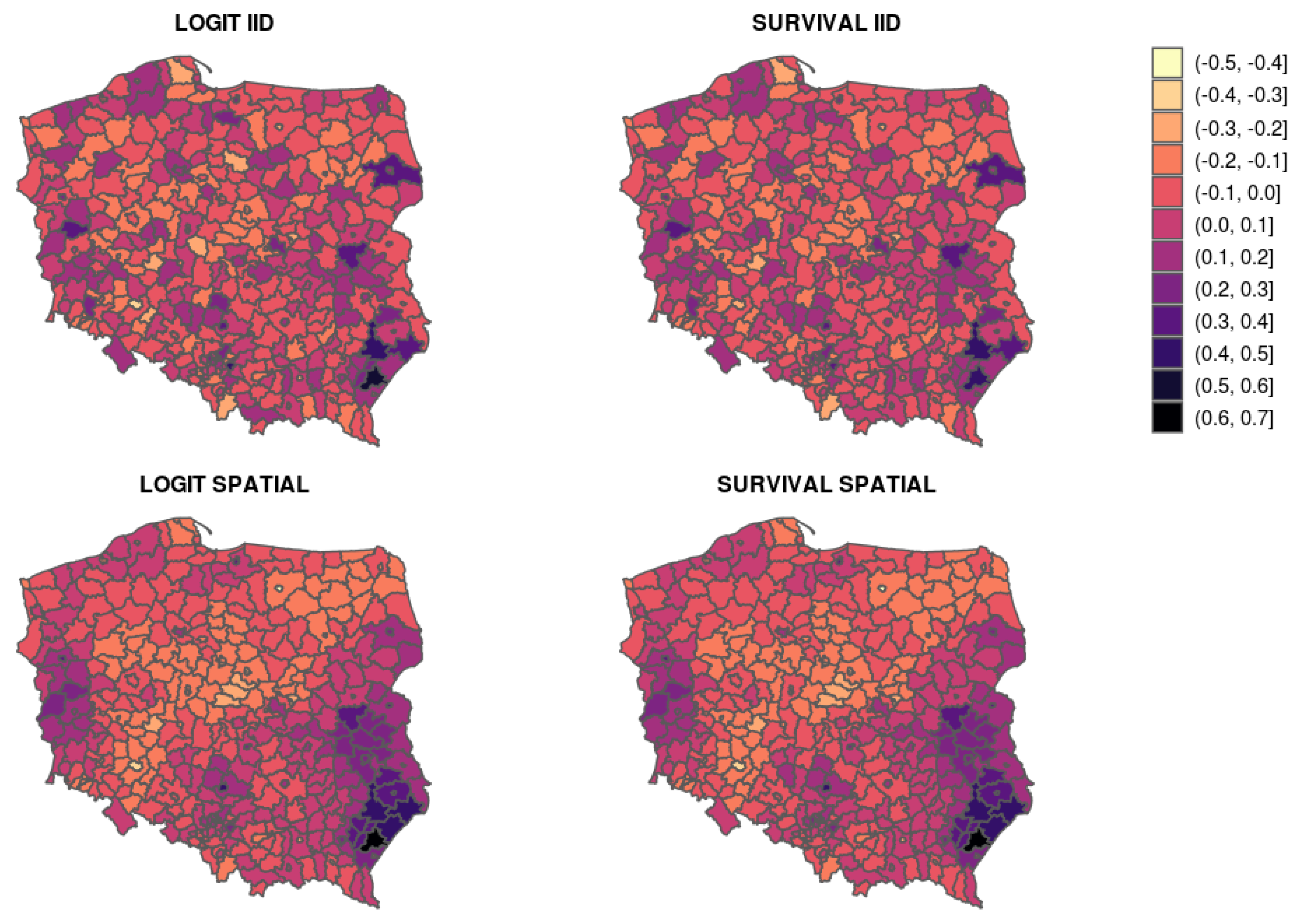
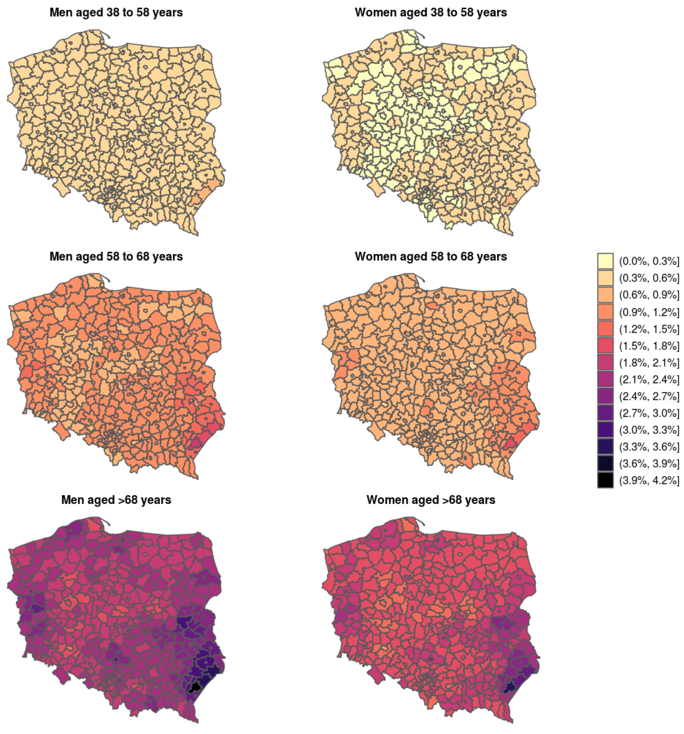
Bayesian Logistic and Survival Modeling

Let $p_{ij}$ be the probability that the individual i living in powiat j will suffer an ischemic stroke, and $T_{ij}$ be the time when that individual suffers a stroke since entering the study. The statistical analysis begins with a basic logistic regression and a basic accelerated failure time survival model for analyzing the probability $p_{ij}$ and the survival time $T_{ij}$, respectively, in terms of covariates gender, age, prescriptions for reimbursed drugs, and PID as follows:

$$\begin{array}{cc}\hfill \mathrm{logit}\left(p_{ij}\right)& ={\mathit{x}}_{ij}^{\prime }\mathit{\beta }\hfill \\ \hfill \log \left(T_{ij}\right)& ={\mathit{x}}_{ij}^{\prime }\mathit{\beta }+\sigma {\mathit{ϵ}}_{ij}\hfill \\ \hfill {\mathit{x}}_{ij}^{\prime }\mathit{\beta }& ={\beta }_0+{\beta }_1{I}_{Woman}\left(ij\right)+{\beta }_2{I}_{Age2}\left(ij\right)+{\beta }_3{I}_{Age3}\left(ij\right)+{\beta }_4{I}_{City}\left(ij\right)+\hfill \\ & +{\beta }_5{I}_{T.A10}\left(ij\right)+{\beta }_6{I}_{T.B01}\left(ij\right)+{\beta }_7{I}_{T.C}\left(ij\right)\left(ij\right)+{\beta }_{8}Depr\left(j\right),\hfill \end{array}$$

(9)

where $I_A\left(ij\right)$ is an indicator variable for A that takes the value 1 if the individual i from powiat j has the characteristic A and zero if she or he does not, and consequently $I_{Woman}\left(ij\right)$, $I_{Age2}\left(ij\right)$, $I_{Age3}\left(ij\right)$, $I_{City}\left(ij\right)$, $I_{T.A10}\left(ij\right)$, $I_{T.B01}\left(ij\right)$ and $I_{T.C}\left(ij\right)$ are the indicator random variables for being a woman, being in age group Age2, Age3, living in city county and having received diabetes, antithrombotic and cardiovascular treatment in powiat j, respectively. The $Depr$ covariate stands for the deprivation index which is the numerical variable defined for each powiat. To complete the specification of the Bayesian model it is necessary to elicit a prior distribution for the parameters and hyperparameters of the model. In the case of the logistic regression model the set of parameters $\mathit{\theta }={({\beta }_0,{\beta }_1,\dots ,{\beta }_8)}^{\prime }$ is a GMRF with diagonal precision matrix 0.001 for all the coefficients except for ${\beta }_0$ whose marginal prior distribution is selected as an improper Gaussian distribution with zero mean and zero precision.

The discussion of the marginal prior distribution for the scale parameter $\sigma$ in the survival model needs a previous comment about INLA and the Weibull distribution. INLA offers two different parameterizations of the Weibull distribution for survival models. We have opted for the so-called first variant, which corresponds to shape parameter $\alpha =1/\sigma$ and scale parameter $\lambda =\exp \left\{{\mathit{x}}_{ij}^{\prime }\mathit{\zeta }\right\}$, so that the hazard function of $T_{ij}$ is

$$h_{ij}\left(t\right)=\lambda \alpha t^{\alpha -1}=\exp \left\{{\mathit{x}}_{ij}^{\prime }\mathit{\zeta }\right\}\alpha t^{\alpha -1}.$$

This parameterization implies that positive coefficients $\zeta$’s of the covariates increase hazard, while negative values reduce it. Note that this parameterization is slightly different from the typical parameterization of this AFT model shown in Equation (7). Coefficients $\zeta$’s estimated with INLA are equal to coefficients $-\beta /\sigma$’s in the accelerated survival model [35].

The shape parameter $\alpha$ of the Weibull distribution has a penalized complexity prior (PC-prior) [36]. In fact, INLA considers $\alpha =\exp \left\{0.1{\alpha }^{\prime }\right\}$ to avoid numerical instabilities and the prior is set on ${\alpha }^{\prime }$. PC-priors are defined using the Kullback–Leibler distance between the proposed model and a natural base model, which in this case corresponds to $\alpha =1$, that is the exponential distribution. In our model, we have used the default PC-prior for $\alpha$; see [37] for details.

Random effects associated with the powiats are introduced in the logistic and the survival model in (9) according to the two proposals presented in the previous section: in terms of conditionally $i.i.d.$ random variables and spatially correlated random variables. The marginal prior distribution of the precision $\tau$ in the case of both conditionally independent and spatially correlated random effects is an improper uniform distribution in the interval 0 to infinity. The weight parameter $\varphi$ in the precision of the spatial effect has a prior distribution so that the logit of $\varphi$ follows a Gaussian distribution with zero mean and precision 0.1.

Table 2. Posterior summaries for the parameters and hyperparameter of the logistic regression model and survival model without random effects (LOGIT and SURVIVAL ), with random effects in terms of conditionally $i.i.d$ random variables (LOGIT IID and SURVIVAL IID ), and spatially correlated random variables (LOGIT SPATIAL and SURVIVAL SPATIAL).

Covariable		Logit	Survival	Logit IID	Survival IID	Logit Spatial	Survival Spatial
Intercept	mean CI	−5.901 (−6.013, −5.791)	−5.902 (−6.014, −5.793)	−5.925 (−6.042, −5.811)	−5.925 (−6.041, −5.811)	−5.912 (−6.061, −5.764)	−5.914 (−6.072, −5.757)
Woman	mean CI	−0.217 (−0.291, −0.142)	−0.214 (−0.288, −0.14)	−0.217 (−0.291, −0.142)	−0.214 (−0.288, −0.14)	−0.216 (−0.291, −0.142)	−0.214 (−0.288, −0.14)
Group Age2 (58−68]	mean CI	0.935 (0.812, 1.058)	0.933 (0.81, 1.056)	0.933 (0.81, 1.057)	0.931 (0.809, 1.055)	0.933 (0.81, 1.057)	0.932 (0.809, 1.055)
Group Age3 (68−108]	mean CI	1.729 (1.613, 1.847)	1.722 (1.606, 1.84)	1.729 (1.612, 1.847)	1.722 (1.605, 1.839)	1.728 (1.611, 1.846)	1.72 (1.604, 1.838)
City county	mean CI	0.122 (−0.015, 0.258)	0.121 (−0.015, 0.256)	0.07 (−0.104, 0.242)	0.07 (−0.1, 0.24)	0.007 (−0.17, 0.184)	0.007 (−0.173, 0.183)
T.A10	mean CI	0.238 (0.149, 0.326)	0.235 (0.147, 0.322)	0.238 (0.149, 0.326)	0.235 (0.147, 0.322)	0.239 (0.15, 0.327)	0.236 (0.148, 0.324)
T.B01	mean CI	0.235 (0.141, 0.328)	0.234 (0.14, 0.326)	0.236 (0.141, 0.329)	0.234 (0.14, 0.326)	0.236 (0.141, 0.329)	0.234 (0.14, 0.326)
T.C	mean CI	0.324 (0.224, 0.425)	0.322 (0.222, 0.423)	0.325 (0.224, 0.426)	0.323 (0.223, 0.424)	0.324 (0.224, 0.425)	0.322 (0.222, 0.423)
Deprivation index	mean CI	0.179 (0.092, 0.265)	0.178 (0.091, 0.263)	0.128 (0.012, 0.243)	0.129 (0.015, 0.242)	0.096 (−0.022, 0.214)	0.095 (−0.025, 0.213)
Precision $\tau$	mean CI			16.833 (11.063, 22.566)	18.562 (13.66, 25.462)	11.306 (8.472, 15.486)	9.365 (4.78, 14.554)
Shape parameter $1/\sigma$	mean CI		1.114 (1.075, 1.155)		1.112 (1.08, 1.149)		1.112 (1.079, 1.147)
Parameter $\varphi$	mean CI					0.866 (0.746, 0.925)	0.889 (0.747, 0.978)
DIC	mean CI	31,296.11	31,263.72	31,258.58	31,225.10	31,231.96	31,200.00
WAIC	mean CI	31,296.14	31,263.49	31,256.18	31,222.83	31,230.30	31,198.86

presents the posterior mean and posterior credible intervals for the parameters and hyperparameters of the logistic regression model and the accelerated survival model without random effects, and with random effects in terms of conditionally $i.i.d$ random variables and spatially correlated random variables. Moreover, all models have been evaluated through the DIC and WAIC criteria. For both types of modeling (i.e., logistic and survival), the model with spatially correlated random effects has the lowest values of DIC and WAIC.

Times required to complete model fitting have been less that 20 min, with survival models taking a slightly shorter times than logit models. Models have been fit on a cluster running Linux with 64-bit 64 Intel(R) Xeon(R) CPU E5-2683 v4 @ 2.10GHz cpus, of which only 16 have been used to fit each model. R version 3.6.3 [24] and INLA 20.12.10 [13] have been used for model fitting.

All models have similar estimates of the regression coefficients associated with the covariates, providing evidence of statistical robustness. As expected, a lower risk of stroke is associated with being a woman and age increases the risk of stroke. Naively, this can be regarded as if the results pointed to that being male increases the stroke rate by about 25% and being in the older age group multiplies the stroke rate by about 5–6 times. The estimates of the model indicate that men older than 68 who live in a city county have the highest risk of stroke. It is worth noting the positive relationship between the pharmacological prescriptions dispensed to patients and the risk of stroke, especially those related to the cardiovascular system. The analysis of the credible intervals suggests that all the covariates, except the county, are relevant both for the risk of stroke and for time to stroke. The risk of stroke grows in proportion to the deprivation index although the importance of this variable is questionable. The posterior mean of the parameter $1/\sigma$ of the survival models is always close to 1. It could suggest that the risk of stroke does increase with time, but not rapidly. This latter may be because the data was collected only for a period of two years and relates to people without specific diseases.

The posterior mean of the hyperparameter $\varphi$ which assesses the strength of the spatial effect in the spatial models is equal to 0.866 and 0.889 for the logistic regression and for the survival model, respectively, with 95% credible intervals that clearly state the relevance of the spatial effect. The posterior mean of the precision $\tau$ estimated for counties indicates that there is variation between powiats. It is lower for the spatial models, but still this is evidence of the dispersion in the data.

Figure 1 illustrates the posterior mean of the random effects for both the logistic regression and the survival modeling. As expected, the outcomes associated with the different powiats in the conditional $i.i.d$ models are very similar to well as those for the two spatial effects models. There are, however, differences between the conditional $i.i.d$ and spatial models. The latter show strong spatial patterns, with a southwest–northeast alignment of the smallest values, which can be interpreted as regions with lower probability of stroke. On the contrary, a high-value cluster in the southeast, means that the risk of stroke is higher than in the other parts of the country.

The potential of the models analyzed is enormous because they allow us to study and visualize the outcomes of interest in relation to the population subgroups defined by the different values of the covariates. This information is too long to be included in this article. By way of illustration, we present in Figure 2 the posterior expectation of the probability of stroke, by gender and age group, for people who did not take any medication, obtained from the spatial logistic regression model. It is clearly visible that the probability of stroke increases with age and in general women have lower probability than men. The largest difference between the estimated values is in the oldest age group. The spatial pattern is very relevant. In the southeast of Poland (Podkarpackie and Lubelskie Voivodeship) there is a visible spatial cluster with the highest risk of stroke. Among the ten powiats with the lowest estimated probabilities of stroke, nine of them are cities including Wroclaw, Cracow and the capital Warsaw. Similarly, and in accordance with the illustrative objective, Figure 3 shows the posterior probabilities of stroke by gender and age group for people who takes drugs for the cardiovascular system (ATC C). The overall pattern shows higher probabilities of stroke than in Figure 2 due to the effect associated with these drugs (and the underlying condition, i.e., cardiovascular diseases).

4. Discussion

As previously stated in this paper, health care decisions often involve the collection and analysis of datasets from different sources. Typical health data include mortality and morbidity of certain diseases as well as other information about risk factors, environmental exposure and others [38]. In addition, statistical developments in recent years allow researchers to handle, both methodologically and computationally, large datasets of individual data for population level analyses that involve highly parameterized hierarchical models [39].

Interesting analysis for health care decisions include the estimation of prevalence, assessment of risk factors, estimation of spatial and temporal risk variation, to mention a few. The assessment of risk factors is particularly important because the identification (and prevention) of relevant risk factors may help to reduce morbidity, which in turn may reduce mortality and public health care expenditure.

Public health authorities can benefit from these population level analyses in different ways. First, insight on a given condition can be gained by conducting a population-wide analysis. Secondly, potential risk factors can be assessed which can help to develop best health policies and practices. In the study developed in this paper, a better understanding of the incidence of stroke in Poland is gained as well as knowledge about potential risk factors, with a particular interest on different conditions and associated prescription drugs. Given that health care decisions by government agencies have an immediate and long-lasting effects on the populations it is important that these decisions are data-driven.

In particular, this paper considers the analysis of population data about stroke disease in Poland in a 2-year period. This is a large dataset that comprises information about 500,000 people on several topics, including age, gender, other conditions and drugs prescribed, region and others. In addition to the individual-level data, information at the powiat level (such as deprivation index and city/land county indicator) are available to complete the analysis. Given the high burden of stroke, identifying risk factors which can lead to a reduction in the prevalence of stroke will have a significant impact on the overall quality of life of the population and the cost of public health care.

The available data can be approached in several different ways. First of all, the probability of suffering from a stroke has been considered, for which a logit analysis has been conducted. However, given that the time-to-stroke is available, survival models can be used as well to tackle an alternative inferential outcome. As individual and area level data are available, multilevel models have been fitted. In addition to the individual and area level covariates, mixed-effect models that include random effects at the area level have been studied in two different ways: conditional independent and spatially correlated random effects.

All these models have been estimated using a Bayesian framework, for which novel computational methods have been used to fit the required models. In particular, the integrated nested Laplace approximation [13] has been used to obtain approximations of the posterior marginals of the parameters, random effects and hyperparameters of the model. In addition, the implementation of INLA in the R-INLA package can handle the hundreds of thousands of records in the dataset and fit the models in a few minutes. One of the main aspects of this work is to show the importance of spatial modelling and Bayesian inference as useful tools to identify spatial, demographic and socio-economic patterns in the distribution of health data in a given population, in this case stroke in Poland.

Relevant risk factors identified by the analysis include age, gender and certain conditions and associated drug prescriptions. In particular, women showed a lower risk, which increased with age. Regarding the prescription drugs, three different types of drugs (associated with relevant health risk factors of stroke) were included in the models and they showed an increase in risk of suffering from a stroke. However, our analysis is not able to disentangle whether this increased risk is due to the condition or the associated treatment. Furthermore, the estimates of both types of random effects showed differences among powiats. Model selection using the DIC and WAIC pointed to the model with fixed effects and spatially correlated random effects as the best one among all the models proposed for both the logit and survival families of models.

These models can be exploited for inference in several ways. The spatial logit model can provide estimates of the probability of suffering a stroke for age, gender and area. Similarly, survival models can provide estimates of time-to-stroke for any individual or the median time-to-stroke according to age, gender and area, and include the effect of prescription drugs in the estimates.

Other similar models can be used in the analysis of this dataset but the proposed models provide additional opportunities for inference. As an example, the output from the fitted models can be used for personalized medicine provided that relevant individual-level information (e.g., genetic markers) is available.

References

1. World Health Organization. The Top 10 Causes of Death. Available online: https://www.who.int/news-room/fact-sheets/detail/the-top-10-causes-of-death (accessed on 31 January 2021).
2. Luengo-Fernandez, R.; Violato, M.; Candio, P.; Leal, J. Economic burden of stroke across Europe: A population-based cost analysis. Eur. Stroke J. 2020, 5, 17–25. [Google Scholar] [CrossRef] [PubMed]
3. Feigin, V.; Norrving, B.; George, M.; Foltz, J.; Roth, G.; Mensah, G. Prevention of stroke: A strategic global imperative. Nat. Rev. Neurol. 2016, 12, 501–512. [Google Scholar] [CrossRef] [PubMed]
4. Mohan, K.; Wolfe, C.; Rudd, A.; Heuschmann, P.; Kolominsky-Rabas, P.; Grieve, A. Risk and cumulative risk of stroke recurrence: A systematic review and meta-analysis. Stroke 2011, 42, 1489–1494. [Google Scholar] [CrossRef] [PubMed] [Green Version]
5. Udary móZgu—Rosnący Problem w Starzejącym Się społEczeństwie; Technical Report; Instytut Ochrony Zdrowia w Polsce: Warszawa, Poland, 2016.
6. An Anonymised Sample of Polish National Health Fund (NFZ) Data on the Occurrence of Ischemic Stroke. Available online: https://dane.gov.pl/pl/dataset/1711 (accessed on 31 January 2021).
7. Bivand, R.S.; Gómez-Rubio, V. Spatial survival modelling of business re-opening after Katrina: Survival modelling compared to spatial probit modelling of re-opening within 3, 6 or 12 months. Stat. Model. 2021, 21, 137–160. [Google Scholar] [CrossRef]
8. Ibrahim, J.G.; Chen, M.H.; Sinha, D. Bayesian Survival Analysis; Springer: New York, NY, USA, 2001. [Google Scholar]
9. Leroux, B.; Lei, X.; Breslow, N. Estimation of Disease Rates in Small Areas: A New Mixed Model for Spatial Dependence. In Statistical Models in Epidemiology, the Environment and Clinical Trials; Halloran, M., Berry, D., Eds.; Springer: New York, NY, USA, 1999; pp. 135–178. [Google Scholar]
10. Banerjee, S.; Wall, M.M.; Carlin, B.P. Frailty modeling for spatially correlated survival data, with application to infant mortality in Minnesota. Biostatistics 2003, 4, 123–142. [Google Scholar] [CrossRef] [PubMed] [Green Version]
11. Aswi, A.; Cramb, S.; Duncan, E.; Hu, W.; White, G.; Mengersen, K. Bayesian Spatial Survival Models for Hospitalisation of Dengue: A Case Study of Wahidin Hospital in Makassar, Indonesia. Int. J. Environ. Res. Public Health 2020, 17, 878. [Google Scholar] [CrossRef] [PubMed] [Green Version]
12. Brooks, S.; Gelman, A.; Jones, G.L.; Meng, X.L. Handbook of Markov Chain Monte Carlo; Chapman & Hall/CRC Press: Boca Raton, FL, USA, 2011. [Google Scholar]
13. Rue, H.; Martino, S.; Chopin, N. Approximate Bayesian inference for latent Gaussian models by using integrated nested Laplace approximations. J. R. Stat. Soc. Ser. B 2009, 71, 319–392. [Google Scholar] [CrossRef]
14. Christensen, R.; Johnson, W.; Branscum, A.; Hanson, T. Bayesian Ideas and Data Analysis: An Introduction for Scientists and Statisticians; Chapman & Hall/CRC Press: Boca Raton, FL, USA, 2011. [Google Scholar]
15. Paciorek, C.J. Computational techniques for spatial logistic regression with large data sets. Computational Statistics & Data Analysis 2007, 51, 3631–3653. [Google Scholar] [CrossRef] [Green Version]
16. Besag, J. Spatial Interaction and the Statistical Analysis of Lattice Systems. J. R. Stat. Soc. Ser. B Methodol. 1974, 36, 192–236. [Google Scholar] [CrossRef]
17. Banerjee, S.; Carlin, B.P.; Gelfand, A.E. Hierarchical Modeling and Analysis for Spatial Data, 2nd ed.; Chapman & Hall/CRC: Boca Raton, FL, USA, 2014. [Google Scholar]
18. Kalbfleisch, J.D.; Prentice, R.L. The Statistical Analysis of Failure Time Data; Wiley: New York, NY, USA, 1980. [Google Scholar]
19. Cox, D.; Oakes, D. Analysis of Survival Data; Chapman & Hall: New York, NY, USA, 1984. [Google Scholar]
20. Bardenet, R.; Doucet, A.; Holmes, C. On Markov chain Monte Carlo methods for tall data. J. Mach. Learn. Res. 2017, 18, 1–43. [Google Scholar]
21. Rue, H.; Held, L. Gaussian Markov Random Fields: Theory and Applications; Chapman & Hall/CRC Press: Boca Raton, FL, USA, 2005. [Google Scholar]
22. Gómez-Rubio, V. Bayesian Inference with INLA; CRC Press/Taylor and Francis: Boca Raton, FL, USA, 2000. [Google Scholar]
23. Martins, T.G.; Simpson, D.; Lindgren, F.; Rue, H. Bayesian computing with INLA: New features. Comput. Stat. Data Anal. 2013, 67, 68–83. [Google Scholar] [CrossRef] [Green Version]
24. R Core Team. R: A Language and Environment for Statistical Computing; R Foundation for Statistical Computing: Vienna, Austria, 2020. [Google Scholar]
25. Spiegelhalter, D.J.; Best, N.G.; Carlin, B.P.; der Linde, A.V. Bayesian Measures of Model Complexity and Fit (with discussion). J. R. Stat. Soc. Ser. B 2002, 64, 583–616. [Google Scholar] [CrossRef] [Green Version]
26. Watanabe, S. A widely applicable Bayesian information criterion. J. Mach. Learn. Res. 2013, 14, 867–897. [Google Scholar]
27. The Burden of Stroke in Europe Report. Technical report, Stroke Alliance for Europe (SAFE). 2017. Available online: https://www.safestroke.eu/burden-of-stroke/ (accessed on 31 January 2021).
28. King, G.; Zeng, L. Logistic Regression in Rare Events Data. Political Anal. 2001, 9, 137–163. [Google Scholar] [CrossRef] [Green Version]
29. Journal of Laws of the Republic of Poland [Dz.U.] of 2002, No. 93, Item 821. Available online: https://dziennikustaw.gov.pl/DU/rok/2002/wydanie/93/pozycja/821 (accessed on 31 January 2021).
30. Journal of Laws of the Republic of Poland [Dz.U.] of 2012, Item 853. Available online: https://dziennikustaw.gov.pl/DU/2012/853 (accessed on 31 January 2021).
31. Boehme, A.K.; Esenwa, C.; Elkind, M.S.V. Stroke Risk Factors, Genetics, and Prevention. Circ. Res. 2017, 120, 472–495. [Google Scholar] [CrossRef] [PubMed]
32. Guidelines for ATC Classification and DDD Assignment, 2021; WHO Collaborating Centre for Drug Statistics Methodology: Oslo, Norway, 2020.
33. Addo, J.; Ayerbe, L.; Mohan, K.; Crichton, S.; Sheldenkar, A.; Chen, R.; Wolfe, C.; McKevitt, C. Socioeconomic status and stroke: An updated review. Stroke 2012, 43, 1186–1191. [Google Scholar] [CrossRef] [PubMed]
34. Smętkowski, M.; Gorzelak, G.; Płoszaj, A.; Rok, J. Poviats Threatened by Deprivation: State, Trends and Prospects; Technical Report; EUROREG Reports and Analyses No. 7/2015; Centre for European Regional and Local Studies EUROREG: Warsaw, Poland, 2015. [Google Scholar] [CrossRef]
35. Wang, X.; Ryan, Y.Y.; Faraway, J.J. Bayesian Regression Modeling with INLA; Chapman and Hall: Boca Raton, FL, USA, 2018. [Google Scholar]
36. Simpson, D.P.; Rue, H.; Riebler, A.; Martins, T.G.; Sørbye, S.H. Penalising model component complexity: A principled, practical approach to constructing priors. Stat. Sci. 2017, 32, 1–28. [Google Scholar] [CrossRef]
37. Van Niekerk, J.; Bakka, H.; Rue, H. A Principled Distance-Based Prior for the Shape of the Weibull Model. arXiv 2020, arXiv:2002.06519. [Google Scholar]
38. The Future of the Public’s Health in the 21st Century; Understanding Population Health and Its Determinants; National Academies Press (US): Washington, DC, USA, 2002; Chapter 2.
39. Bates, D.; Saria, S.; Ohno-Machado, L.; Shah, A.; Escobar, G. Big data in health care: Using analytics to identify and manage high-risk and high-cost patients. Health Aff. Proj. Hope 2014, 33, 1123–1131. [Google Scholar] [CrossRef] [PubMed] [Green Version]
Figure 1. Posterior mean for the conditional i . i . d random variables in LOGIT IID and SURVIVAL IID models, and for spatially correlated random variables in LOGIT SPATIAL and SURVIVAL models.
Mathematics 09 00577 g001
Figure 2. Estimated probability of stroke by gender and age group based on the LOGIT SPATIAL model.
Mathematics 09 00577 g002
Figure 3. Estimated probability of stroke by gender and age group based on the LOGIT SPATIAL model assuming that drugs for the cardiovascular system (ATC C) have been prescribed.
Mathematics 09 00577 g003