Unpredictable Oscillations for Hopfield-Type Neural Networks with Delayed and Advanced Arguments

Abstract

This is the first time that the method for the investigation of unpredictable solutions of differential equations has been extended to unpredictable oscillations of neural networks with a generalized piecewise constant argument, which is delayed and advanced. The existence and exponential stability of the unique unpredictable oscillation are proven. According to the theory, the presence of unpredictable oscillations is strong evidence for Poincaré chaos. Consequently, the paper is a contribution to chaos applications in neuroscience. The model is inspired by chaotic time-varying stimuli, which allow studying the distribution of chaotic signals in neural networks. Unpredictable inputs create an excitation wave of neurons that transmit chaotic signals. The technique of analysis includes the ideas used for differential equations with a piecewise constant argument. The results are illustrated by examples and simulations. They are carried out in MATLAB Simulink to demonstrate the simplicity of the diagrammatic approaches.

1. Introduction

There are hybrid neural networks, which are neither continuous-time nor purely discrete-time, and among them are dynamical systems with impulses and models with piecewise constant arguments [1,2,3,4,5,6,7,8,9,10]. In recent years, the dynamics of Hopfield-type neural networks have been studied and developed by many authors by using impulsive differential equations [11,12,13,14,15] and differential equations with a piecewise constant argument [16,17,18,19]. In this paper, a new model of Hopfield-type neural networks with an unpredictable input-output, as well as a delayed and advanced generalized piecewise constant argument is proposed. Hopfield-type neural networks are effective at adaptive pattern recognition and vision and image processing [20,21,22]. Differential equations with a piecewise constant argument describing the Hopfield neural networks may “memorize” the values of the phase variable at certain moments of time to utilize the values during the middle process till the next moment [5,6,7,8,9,10,16,17,18,19,23,24,25,26,27,28]. Neural networks, comprised of chaotically oscillating elements, store and transmit information in almost the same way as nerve cells in the brain. It is known that unpredictable oscillations cause chaotic behavior [29,30,31,32,33,34,35,36,37,38,39,40,41]. Therefore, their presence is necessary to study chaotic dynamics in neural networks.

The novelty of our results has to be considered with respect to oscillations, chaos, and modeling for neural networks. Oscillations such as periodic and almost periodic were discussed intensively in [16,17,18,19,23,24,25,26,27,42,43,44,45]. However, the most developed are unpredictable oscillations, which were introduced and developed in [31,32,33,34,35,36,37,38,39]. This is the first time unpredictable oscillations have been considered for neural networks with a generalized-type piecewise constant argument. The argument admits the property to be delayed and advanced, and consequently, it provides rich opportunities for the investigation and application of neural networks.

It is known that oscillations and periodic motions are frequently observed in the activities of the neurons in the brain. Recent developments in the field of neural networks have led to an increased interest in the complexity of the dynamics. Oscillations and chaos in neural networks are actual and have stimulated the interest of many scientists [46,47,48,49,50]. They occur in a neural network system due to the properties of single neurons [46,50,51] and synaptic connections among neurons [52,53]. Neural networks in present research display unpredictable oscillations and chaos. The unpredictable function was introduced in [29] and is based on the dynamics of unpredictable points and Poincaré chaos [30]. More precisely, the function is an unpredictable point of the Bebutov dynamics, and consequently, it is a member of the chaotic set [31]. The notion of the unpredictable point extends the frontiers of the classical theory of dynamical systems, and the unpredictable function provides new problems of the existence of unpredictable oscillations for the theory of differential equations [29,30,31,32,33,34,35,36]. These studies have been identified as major contributing factors for the emergence of new types of sophisticated motion. Significant results have been obtained for unpredictable oscillations of Hopfield-type neural networks, shunting inhibitory cellular neural networks, and inertial neural networks [37,38,39].

To the best of our knowledge, there have been very few results on the dynamical behavior of Hopfield-type neural networks with piecewise constant arguments [16,17,18,19,26,27]. In the present paper, we try to expand them by considering piecewise constant arguments of the generalized type [5,6,7,8,9,10,16,17,18,19,23,24,25,26,27,28,43,44] and by using the theory of unpredictable functions. We improve on previous methods by considering unpredictable inputs, which allow studying the distribution of chaotic signals in neural networks.

2. Preliminaries

Denote by $\mathbb{R},\mathbb{N},\mathbb{Z}$ the set of all real numbers, natural numbers, and integers, respectively. Introduce a norm for the vector $u=(u_1,\cdots ,u_m),$ $u_i\in \mathbb{R},$ $i=1,\cdots ,m,$ as ${\displaystyle \left|\right|u\left|\right|=\underset{1\le i\le m}{max}\left|u_i\right|,}$ where $|·|$ is the absolute value. Correspondingly, for a square matrix $A={\left(a_{ij}\right)}_{m\times m}$, the norm ${\displaystyle \parallel A\parallel =\underset{1\le i\le m}{max}\sum _{j=1}^m\left|a_{ij}\right|}$ is utilized.

We fix two real valued sequences ${\theta }_i,{\xi }_i,i\in \mathbb{Z},$ such that ${\theta }_i<{\theta }_{i+1},{\theta }_i\le {\xi }_i\le {\theta }_{i+1}$ for all $i\in \mathbb{Z},|{\theta }_i|\to \infty$ as $\left|i\right|\to \infty .$ It is assumed that there exists a positive number $\theta$ such that ${\theta }_{k+1}-{\theta }_k\le \theta$ for all integers k.

The main subject under investigation in this paper is the following Hopfield-type neural network system with a piecewise constant argument:

$${\displaystyle x_i^{\prime }\left(t\right)=-a_i{x}_i\left(t\right)+\sum _{j=1}^m{b}_{ij}{f}_j\left(x_j\left(t\right)\right)+\sum _{j=1}^m{c}_{ij}{g}_j\left(x_j\left(\gamma \left(t\right)\right)\right)+{\vartheta }_i\left(t\right),}$$

(1)

where $t,x_i\in \mathbb{R},i=1,2,\dots m,\gamma \left(t\right)={\xi }_k$ if ${\theta }_k\le t<{\theta }_{k+1},k\in \mathbb{Z}:$

• $a_i>0$—the rates with which the units self-regulate or reset their potentials when isolated from other units and inputs;
• m—the number of neurons in the network;
• $x_i\left(t\right)$—the state of the ith unit at time t;
• $f_j$, $g_j$—the activation functions of the incoming potentials of the unit j;
• $b_{ij},c_{ij}$—the synaptic connection weights of the unit j on the unit i;
• ${\vartheta }_i\left(t\right)$—the time-varying stimulus, corresponding to the external input from outside the network to the unit i.

Throughout this paper, we assume that the parameters $b_{ij}$ and $c_{ij}$ are real and that the activation functions $f_j,g_j:\mathbb{R}\to \mathbb{R}j=1,2,\dots ,m$ are continuous functions. Moreover, suppose that there exist positive constants $\lambda$ and $\overline{\lambda }$ such that the inequality $\lambda \le a_i\le \overline{\lambda },$ holds for each $i=1,2,\dots ,m$.

We present system (1) in the following vector form:

$$x^{\prime }\left(t\right)=Ax\left(t\right)+Bf\left(x\left(t\right)\right)+Cg\left(x\left(\gamma \left(t\right)\right)\right)+\vartheta \left(t\right),$$

(2)

where $x=colon(x_1,x_2,\dots ,x_m)$ is the neuron state vector, $f\left(x\right)=colon(f_1\left(x_1\right),$ $f_2\left(x_2\right),\dots ,f_m\left(x_m\right))$ and $g\left(x\right)=colon(g_1\left(x_1\right),g_2\left(x_2\right),\dots ,g_m\left(x_m\right))$ are the activations, and $\vartheta =colon({\vartheta }_1,{\vartheta }_2,\dots ,{\vartheta }_m)$ is the input vector. Moreover, $A=diag(-a_1,-a_2,\dots ,-a_m)$, $B={\left(b_{ij}\right)}_{m\times m}$, $C={\left(c_{ij}\right)}_{m\times m}$ are matrices.

As the usual activations for continuous time neural network dynamics, the following sigmoidal functions are considered [45]:

$$\begin{array}{ccc}\hfill & & f\left(\sigma \right)=tanh\left(\sigma \right)=\frac{e^{\sigma }-e^{-\sigma }}{e^{\sigma }+e^{-\sigma }},\hfill \\ & & f\left(\sigma \right)=\frac{2}{\pi }arctan\left(\frac{2\sigma }{\pi }\right).\hfill \end{array}$$

They are used in neural networks as activation functions, since they allow both amplifying weak signals and do not become saturated by strong signals. The activation function and the output function are summed up with the term transfer functions. If the activation function determines the total signal a neuron receives, the transfer function translates the input signals to the output signals.

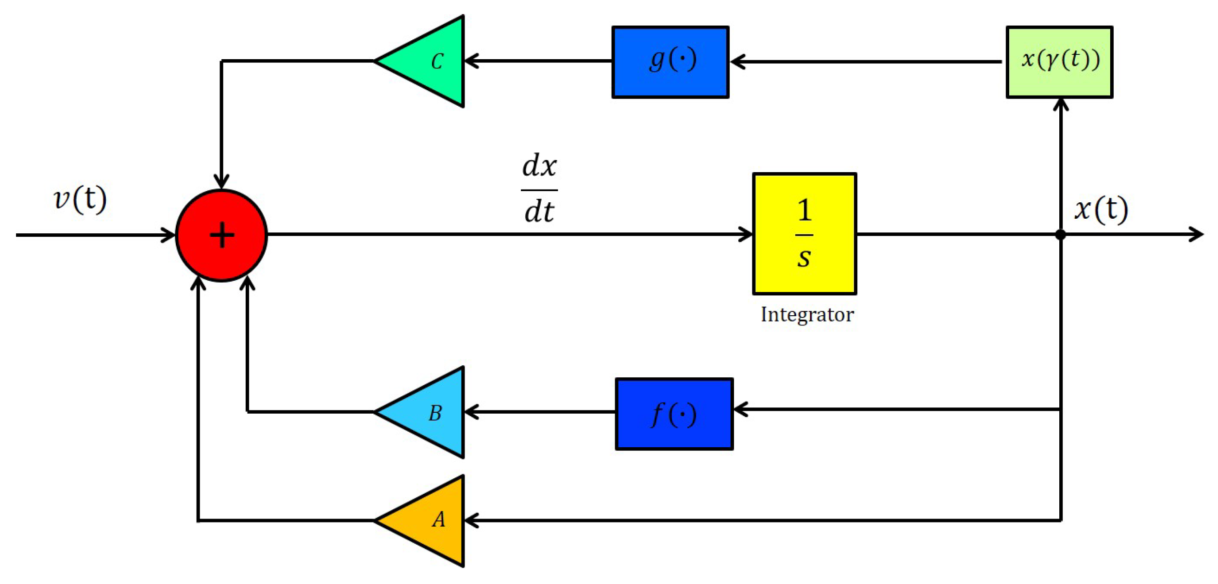
The block diagram of the Hopfield-type neural network system with a piecewise constant argument is shown in Figure 1, and the symbols for the diagram are described in

Table 1. Characteristics of elements of the block diagram in Figure 1.

Symbols	Description
	Integrator block
	Sum block
	Gain blocks, with values $A,B,C$
	Transfer function block, with nonlinear functions f and g
	MATLAB function block, with the piecewise constant function $\gamma \left(t\right)$
$\vartheta \left(t\right)$	Input function
$x\left(t\right)$	Output function

.

Definition 1

([29]). A uniformly continuous and bounded function $v:\mathbb{R}\to {\mathbb{R}}^m$ is unpredictable if there exist positive numbers ${ϵ}_0,\delta$ and sequences $t_n,u_n$, both of which diverge to infinity such that $v(t+t_n)\to v\left(t\right)$ as $n\to \infty$ uniformly on compact subsets of $\mathbb{R}$ and $\parallel v(t+t_n)-v\left(t\right)\parallel \ge {ϵ}_0$ for each $t\in [u_n-\delta ,u_n+\delta ]$ and $n\in \mathbb{N}$.

3. Main Results

Let ${\mathsf{\Sigma }}_0$ denote the space of m-dimensional vector-functions $\phi :\mathbb{R}\to {\mathbb{R}}^m$, $\phi =({\phi }_1,{\phi }_2,\dots ,{\phi }_m)$ with the norm ${\parallel \phi \parallel }_1=\underset{t\in \mathbb{R}}{sup}∥\phi \left(t\right)∥.$ The functions of this space are assumed to satisfy the following properties:

(A1)

they are uniformly continuous;

(A2)

there exists a number $H>0$ such that ${\parallel \phi \parallel }_1<H$ for each function $\phi$;

(A3)

there exists a sequence $t_n$ that diverges to infinity such that $\phi (t+t_n)\to \phi \left(t\right)$ uniformly on each closed and bounded interval of the real axis for each function $\phi$.

The following conditions on the system (2) are assumed:

(C1)

$\parallel f\left(u\right)-f\left(v\right)\parallel \le L\parallel u-v\parallel$ and $\parallel g\left(u\right)-g\left(v\right)\parallel \le \overline{L}\parallel u-v\parallel$ for all $u,v\in {\mathbb{R}}^m,$ where $L,\overline{L}$ are positive constants;

(C2)

there exist positive numbers $m_f$, $m_g$ such that $\underset{\parallel x\parallel <H}{sup}∥f\left(x\right)∥\le m_f$ and $\underset{\parallel x\parallel <H}{sup}∥g\left(x\right)∥\le m_g$;

(C3)

$\vartheta$ is a function from the space ${\Sigma }_0$, and there exists a positive number $m_{\vartheta }$ such that $\underset{t\in \mathbb{R}}{sup}∥\vartheta \left(t\right)∥\le m_{\vartheta };$

(C4)

$\parallel B\parallel m_f+\parallel C\parallel m_g+m_{\vartheta }<H\lambda ;$

(C5)

$\parallel B\parallel L+\parallel C\parallel \overline{L}<\lambda ;$

(C6)

$-\lambda +\parallel B\parallel L+K\parallel C\parallel \overline{L}<0$, where

$K={\left(1-\theta \left[\right(\overline{\lambda }+\left|\right|B\left|\right|L\left)\right(1+\left|\right|C\left|\right|\overline{L}\theta )e^{(\overline{\lambda }+|\left|B\right|\left|L\right)\theta }+\left|\right|C\left|\right|\overline{L}]\right)}^{-1}$;

(C7)

$\theta \left[\right(\overline{\lambda }+\left|\right|B\left|\right|L\left)\right(1+\left|\right|C\left|\right|\overline{L}\theta )e^{(\overline{\lambda }+|\left|B\right|\left|L\right)\theta }+\left|\right|C\left|\right|\overline{L}]<1$;

(C8)

there exists a sequence ${\eta }_n$ with the property ${\eta }_n\to \infty$ as $n\to \infty$ such that ${\theta }_{k-{\eta }_n}+t_n-{\theta }_k\to 0$ and ${\xi }_{k-{\eta }_n}+t_n-{\xi }_k\to 0$ as $n\to \infty$ on each finite interval of integers, where $t_n$ is the sequence given in Definition 1.

Lemma 1

([10]). A function $x\left(t\right)=(x_1\left(t\right),\dots ,x_m\left(t\right))$ is a bounded solution of Equation (1) if and only if it is a solution of the following integral equation:

$$\begin{array}{c}{\displaystyle x\left(t\right)=\underset{-\infty }{\overset{t}{\int }}{e}^{A(t-s)}\left[Bf\left(x\right(s\left)\right)+Cg\left(x\right(\gamma \left(s\right)\left)\right)+\vartheta \left(s\right)\right]ds.}\hfill \end{array}$$

(3)

Let us introduce the operator $\Pi$ on ${\Sigma }_0$ such that:

$$\Pi \phi \left(t\right)=\underset{-\infty }{\overset{t}{\int }}{e}^{A(t-s)}\left[Bf\left(\phi \right(s\left)\right)+Cg\left(\phi \right(\gamma \left(s\right)\left)\right)+\vartheta \left(s\right)\right]ds.$$

Lemma 2.

$\Pi {\Sigma }_0\subseteq {\Sigma }_0.$

Proof. 

Let us evaluate the derivative of $\Pi \phi \left(t\right)$ with respect to the time variable $t.$ Then, we have:

$$\begin{array}{ccc}\hfill d\Pi \phi \left(t\right)/dt& =& Bf\left(\phi \right(t\left)\right)+Cg\left(\phi \right(\gamma \left(t\right)\left)\right)+\vartheta \left(t\right)+\hfill \\ & +& A\underset{-\infty }{\overset{t}{\int }}{e}^{A(t-s)}\left[Bf\left(\phi \right(s\left)\right)+Cg\left(\phi \right(\gamma \left(s\right)\left)\right)+\vartheta \left(s\right)\right]ds.\hfill \end{array}$$

Hence, we can find for all $t\in \mathbb{R}$ that:

$$\begin{array}{ccc}\hfill ∥d\Pi \phi \left(t\right)/dt∥& \le & \parallel B\parallel ∥f\left(\phi \right(t\left)\right)∥+\parallel C\parallel ∥g\left(\phi \right(\gamma \left(t\right)\left)\right)∥+∥\vartheta \left(t\right)∥+\hfill \\ & +& \overline{\lambda }\underset{-\infty }{\overset{t}{\int }}{e}^{-\lambda (t-s)}\left[\parallel B\parallel ∥f\left(\phi \right(t\left)\right)∥+\parallel C\parallel ∥g\left(\phi \right(\gamma \left(t\right)\left)\right)∥+∥\vartheta \left(t\right)∥\right]ds\hfill \\ & \le & \parallel B\parallel m_f+\parallel C\parallel m_g+m_{\vartheta }+\overline{\lambda }/\lambda \left(\parallel B\parallel m_f+\parallel C\parallel m_g+m_{\vartheta }\right)\hfill \\ & =& (1+\overline{\lambda }/\lambda )\left(\parallel B\parallel m_f+\parallel C\parallel m_g+m_{\vartheta }\right).\hfill \end{array}$$

Since the derivative of $\Pi \phi \left(t\right)$ is bounded, $\Pi \phi$ is uniformly continuous. This means that $\Pi \phi$ satisfies the property (A1).

Moreover, we have for $\phi \in {\Sigma }_0$ that:

$$\begin{array}{ccc}\hfill \parallel \Pi \phi \left(t\right)\parallel & \le & \underset{-\infty }{\overset{t}{\int }}{e}^{-\lambda (t-s)}\left[\parallel B\parallel \parallel f\left(\phi \right(s\left)\right)\parallel +\parallel C\parallel \parallel g\left(\phi \right(\gamma \left(s\right)\left)\right)\parallel +\parallel \vartheta \left(s\right)\parallel \right]ds\hfill \\ & \le & \underset{-\infty }{\overset{t}{\int }}{e}^{-\lambda (t-s)}\left[\parallel B\parallel m_f+\parallel C\parallel m_g+m_{\vartheta }\right]ds\hfill \\ & \le & {\lambda }^{-1}\left(\parallel B\parallel m_f+\parallel C\parallel m_g+m_{\vartheta }\right).\hfill \end{array}$$

The last inequality together with the condition (C4) implies that ${\left|\right|\Pi \phi \left|\right|}_1<H.$ Thus, $\Pi \phi$ satisfies the property (A2).

Now, we need to check the last property (A3) for $\Pi \phi$. In other words, we have to verify that there exists a sequence $t_n$ that diverges to infinity such that for each $\Pi \phi \in {\Sigma }_0,$ $\Pi \phi (t+t_n)\to \Pi \phi \left(t\right)$ uniformly on each closed and bounded interval of the real axis. Fix an arbitrary positive number $\epsilon$ and a closed interval $[a,b],$ where $a,b\in \mathbb{R}$ with $a<b$. It is enough to show that $\left|\right|\Pi \phi (t+t_n)-\Pi \phi \left(t\right)\left|\right|<\epsilon$ for sufficiently large n and $t\in [a,b].$ We choose two numbers $c<a$ and $ϵ>0$ such that:

$$2{\lambda }^{-1}\left[\parallel B\parallel LH+\parallel C\parallel \overline{L}H+m_{\vartheta }\right]e^{-\lambda (a-c)}<\epsilon /3,$$

(4)

$$ϵ{\lambda }^{-1}\left[1+\parallel B\parallel L\right]<\epsilon /3,$$

(5)

$$2{\lambda }^{-1}\left((p+1)ϵ+pH\right)(1-e^{-\lambda \theta })\parallel C\parallel \overline{L}<\epsilon /3.$$

(6)

Take n large enough such that $\parallel \phi (t+t_n)-\phi \left(t\right)\parallel <ϵ$ and $\parallel \vartheta (t+t_n)-\vartheta \left(t\right)\parallel <ϵ$ on $[c,b]$. Then, for $\phi \in {\Sigma }_0$, by writing:

$$\begin{array}{ccc}\hfill \Pi \phi (t+t_n)-\Pi \phi \left(t\right)& =& {\displaystyle \underset{-\infty }{\overset{t+t_n}{\int }}{e}^{A(t+t_n-s)}\left[Bf\left(\phi \right(s\left)\right)+Cg\left(\phi \right(\gamma \left(s\right)\left)\right)+\vartheta \left(s\right)\right]ds}\hfill \\ & -& \underset{-\infty }{\overset{t}{\int }}{e}^{A(t-s)}\left[Bf\left(\phi \right(s\left)\right)+Cg\left(\phi \right(\gamma \left(s\right)\left)\right)+\vartheta \left(s\right)\right]ds\hfill \\ & =& {\displaystyle \underset{-\infty }{\overset{t}{\int }}{e}^{A(t-s)}[B[f\left(\phi (s+t_n)\right)-f\left(\phi \left(s\right)\right)]}\hfill \\ & +& C[g\left(\phi \left(\gamma (s+t_n)\right)\right)-g\left(\phi \left(\gamma \left(s\right)\right)\right)]+\vartheta (s+t_n)-\vartheta \left(s\right)]ds,\hfill \end{array}$$

one can see that:

$$\begin{array}{ccc}\hfill \parallel \Pi \phi (t+t_n)-\Pi \phi \left(t\right)\parallel & \le & \underset{-\infty }{\overset{t}{\int }}{e}^{-\lambda (t-s)}[\parallel B\parallel L\parallel \phi (s+t_n)-\phi \left(s\right)\parallel \hfill \\ & +& \parallel C\parallel \overline{L}\parallel \phi \left(\gamma (s+t_n)\right)-\phi \left(\gamma \left(s\right)\right)\parallel +\parallel \vartheta (s+t_n)-\vartheta \left(s\right)\parallel ]ds\hfill \end{array}$$

is valid. If we divide the last integral into two parts, we get for $t\in [a,b]$ that:

$$\begin{array}{ccc}\hfill \parallel \Pi \phi (t+t_n)-\Pi \phi \left(t\right)\parallel & \le & {\displaystyle \underset{-\infty }{\overset{c}{\int }}{e}^{-\lambda (t-s)}[\parallel B\parallel L\parallel \phi (s+t_n)-\phi \left(s\right)\parallel }\hfill \\ & +& \parallel C\parallel \overline{L}\parallel \phi \left(\gamma (s+t_n)\right)-\phi \left(\gamma \left(s\right)\right)\parallel \hfill \\ & +& \parallel \vartheta (s+t_n)-\vartheta \left(s\right)\parallel ]ds\hfill \\ & +& {\displaystyle \underset{c}{\overset{t}{\int }}{e}^{-\lambda (t-s)}[\parallel B\parallel L\parallel \phi (s+t_n)-\phi \left(s\right)\parallel }\hfill \\ & +& \parallel C\parallel \overline{L}\parallel \phi \left(\gamma (s+t_n)\right)-\phi \left(\gamma \left(s\right)\right)\parallel \hfill \\ & +& \parallel \vartheta (s+t_n)-\vartheta \left(s\right)\parallel ]ds\hfill \\ & \le & 2{\lambda }^{-1}\left[\parallel B\parallel LH+\parallel C\parallel \overline{L}H+m_{\vartheta }\right]e^{-\lambda (a-c)}\hfill \\ & +& {\displaystyle \underset{c}{\overset{t}{\int }}{e}^{-\lambda (t-s)}[1+\parallel B\parallel L]ϵds}\hfill \\ & +& {\displaystyle \underset{c}{\overset{t}{\int }}{e}^{-\lambda (t-s)}\parallel C\parallel \overline{L}\parallel \phi \left(\gamma (s+t_n)\right)-\phi \left(\gamma \left(s\right)\right)\parallel ds}\hfill \\ & \le & 2{\lambda }^{-1}\left[\parallel B\parallel LH+\parallel C\parallel \overline{L}H+m_{\vartheta }\right]e^{-\lambda (a-c)}\hfill \\ & +& {\lambda }^{-1}[1+\parallel B\parallel L]ϵ\hfill \\ & +& {\displaystyle \underset{c}{\overset{t}{\int }}{e}^{-\lambda (t-s)}\parallel C\parallel \overline{L}\parallel \phi \left(\gamma (s+t_n)\right)-\phi \left(\gamma \left(s\right)\right)\parallel ds}\hfill \\ & \le & 2{\lambda }^{-1}\left[\parallel B\parallel LH+\parallel C\parallel \overline{L}H+m_{\vartheta }\right]e^{-\lambda (a-c)}\hfill \\ & +& {\lambda }^{-1}[1+\parallel B\parallel L]ϵ\hfill \\ & +& {\displaystyle \parallel C\parallel \overline{L}\underset{c}{\overset{t}{\int }}{e}^{-\lambda (t-s)}\parallel \phi \left(\gamma (s+t_n)\right)-\phi \left(\gamma \left(s\right)\right)\parallel ds.}\hfill \end{array}$$

We need to find an upper bound for the last integral. For this purpose, we shall evaluate it by dividing the interval of integration into subintervals as follows. For a fixed $t\in [a,b]$, we assume without loss of generality that ${\theta }_i\le {\theta }_{i-{\eta }_n}+t_n$ and ${\theta }_i\le {\theta }_{i-{\eta }_n}+t_n=c<{\theta }_{i+1}<{\theta }_{i+2}<\cdots <{\theta }_{i+p}\le {\theta }_{i+p-{\eta }_n}+t_n\le t<{\theta }_{i+p+1}$ so that there exist exactly p discontinuity moments in the interval $[c,t].$

Let us denote:

$${\displaystyle I=\underset{c}{\overset{t}{\int }}{e}^{-\lambda (t-s)}\parallel \phi \left(\gamma (s+t_n)\right)-\phi \left(\gamma \left(s\right)\right)\parallel ds.}$$

We shall need the following presentation of the last integral.

$$\begin{array}{ccc}\hfill I& =& {\displaystyle \underset{c}{\overset{{\theta }_{i+1}}{\int }}{e}^{-\lambda (t-s)}\parallel \phi \left(\gamma (s+t_n)\right)-\phi \left(\gamma \left(s\right)\right)\parallel ds}\hfill \\ & +& {\displaystyle \underset{{\theta }_{i+1}}{\overset{{\theta }_{i+1-{\eta }_n}+t_n}{\int }}{e}^{-\lambda (t-s)}\parallel \phi \left(\gamma (s+t_n)\right)-\phi \left(\gamma \left(s\right)\right)\parallel ds}\hfill \\ & +& {\displaystyle \underset{{\theta }_{i+1-{\eta }_n}+t_n}{\overset{{\theta }_{i+2}}{\int }}{e}^{-\lambda (t-s)}\parallel \phi \left(\gamma (s+t_n)\right)-\phi \left(\gamma \left(s\right)\right)\parallel ds}\hfill \\ & +& {\displaystyle \underset{{\theta }_{i+2}}{\overset{{\theta }_{i+2-{\eta }_n}+t_n}{\int }}{e}^{-\lambda (t-s)}\parallel \phi \left(\gamma (s+t_n)\right)-\phi \left(\gamma \left(s\right)\right)\parallel ds}\hfill \\ & +& {\displaystyle \underset{{\theta }_{i+2-{\eta }_n}+t_n}{\overset{{\theta }_{i+3}}{\int }}{e}^{-\lambda (t-s)}\parallel \phi \left(\gamma (s+t_n)\right)-\phi \left(\gamma \left(s\right)\right)\parallel ds}\hfill \\ & ⋮& \\ & +& {\displaystyle \underset{{\theta }_{i+p-{\eta }_n}+t_n}{\overset{t}{\int }}{e}^{-\lambda (t-s)}\parallel \phi \left(\gamma (s+t_n)\right)-\phi \left(\gamma \left(s\right)\right)\parallel ds}\hfill \\ & =& {\displaystyle \sum _{k=i}^{i+p-1}\underset{{\theta }_{k-{\eta }_n}+t_n}{\overset{{\theta }_{k+1}}{\int }}{e}^{-\lambda (t-s)}\parallel \phi \left(\gamma (s+t_n)\right)-\phi \left(\gamma \left(s\right)\right)\parallel ds}\hfill \\ & +& {\displaystyle \sum _{k=i}^{i+p-1}\underset{{\theta }_{k+1}}{\overset{{\theta }_{k+1-{\eta }_n}+t_n}{\int }}{e}^{-\lambda (t-s)}\parallel \phi \left(\gamma (s+t_n)\right)-\phi \left(\gamma \left(s\right)\right)\parallel ds}\hfill \\ & +& {\displaystyle \underset{{\theta }_{i+p-{\eta }_n}+t_n}{\overset{t}{\int }}{e}^{-\lambda (t-s)}\parallel \phi \left(\gamma (s+t_n)\right)-\phi \left(\gamma \left(s\right)\right)\parallel ds.}\hfill \end{array}$$

Now, if we define the integrals in the last expression as:

$${\displaystyle A_k=\underset{{\theta }_{k-{\eta }_n}+t_n}{\overset{{\theta }_{k+1}}{\int }}{e}^{-\lambda (t-s)}\parallel \phi \left(\gamma (s+t_n)\right)-\phi \left(\gamma \left(s\right)\right)\parallel ds}$$

and:

$${\displaystyle B_k=\underset{{\theta }_{k+1}}{\overset{{\theta }_{k+1-{\eta }_n}+t_n}{\int }}{e}^{-\lambda (t-s)}\parallel \phi \left(\gamma (s+t_n)\right)-\phi \left(\gamma \left(s\right)\right)\parallel ds,}$$

where $k=i,i+1,\cdots ,i+p-1,$ then we can write that:

$${\displaystyle I=\sum _{k=i}^{i+p-1}{A}_k+\sum _{k=i}^{i+p-1}{B}_k+\underset{{\theta }_{i+p-{\eta }_n}+t_n}{\overset{t}{\int }}{e}^{-\lambda (t-s)}\parallel \phi \left(\gamma (s+t_n)\right)-\phi \left(\gamma \left(s\right)\right)\parallel ds.}$$

For $t\in [{\theta }_{k-{\eta }_n}+t_n,{\theta }_{k+1}),$ $\gamma \left(t\right)={\xi }_k$, and we have by the condition (C8) that $\gamma (t+t_n)={\xi }_{k+{\eta }_n},$ $k=i,i+1,\cdots ,i+p-1.$ Hence, we obtain that:

$$\begin{array}{ccc}\hfill A_k& =& {\displaystyle \underset{{\theta }_{k-{\eta }_n}+t_n}{\overset{{\theta }_{k+1}}{\int }}{e}^{-\lambda (t-s)}\parallel \phi \left({\xi }_{k+{\eta }_n}\right)-\phi \left({\xi }_k\right)\parallel ds}\hfill \\ & =& {\displaystyle \underset{{\theta }_{k-{\eta }_n}+t_n}{\overset{{\theta }_{k+1}}{\int }}{e}^{-\lambda (t-s)}\parallel \phi ({\xi }_k+t_n+o\left(1\right))-\phi \left({\xi }_k\right)\parallel ds}\hfill \\ & =& {\displaystyle \underset{{\theta }_{k-{\eta }_n}+t_n}{\overset{{\theta }_{k+1}}{\int }}{e}^{-\lambda (t-s)}\parallel \phi ({\xi }_k+t_n)-\phi \left({\xi }_k\right)+\phi ({\xi }_k+t_n+o\left(1\right))-\phi ({\xi }_k+t_n)\parallel ds}\hfill \\ & \le & {\displaystyle \underset{{\theta }_{k-{\eta }_n}+t_n}{\overset{{\theta }_{k+1}}{\int }}{e}^{-\lambda (t-s)}[\parallel \phi ({\xi }_k+t_n)-\phi \left({\xi }_k\right)\parallel +\parallel \phi ({\xi }_k+t_n+o\left(1\right))-\phi ({\xi }_k+t_n)\parallel ]ds}\hfill \\ & \le & {\displaystyle \underset{{\theta }_{k-{\eta }_n}+t_n}{\overset{{\theta }_{k+1}}{\int }}{e}^{-\lambda (t-s)}\left[ϵ+\parallel \phi ({\xi }_k+t_n+o\left(1\right))-\phi ({\xi }_k+t_n)\parallel \right]ds.}\hfill \end{array}$$

Since the function $\phi$ is uniformly continuous, for large n and $ϵ>0$, we can find a $\rho >0$ such that $\parallel \phi ({\xi }_k+t_n+o\left(1\right))-\phi ({\xi }_k+t_n)\parallel <ϵ$ if $|{\xi }_{k+{\eta }_n}-{\xi }_k-t_n|<\rho .$ As a result of this discussion, we conclude that:

$${\displaystyle A_k\le 2ϵ\underset{{\theta }_{k-1-{\eta }_n}+t_n}{\overset{{\theta }_k}{\int }}{e}^{-\lambda (t-s)}ds\le 2ϵ{\lambda }^{-1}(1-e^{-\lambda \theta }).}$$

Moreover, we have by the condition (C8) that:

$${\displaystyle B_k\le 2H\underset{{\theta }_k}{\overset{{\theta }_{k-{\eta }_n}+t_n}{\int }}{e}^{-\lambda (t-s)}ds\le 2H{\lambda }^{-1}(1-e^{-\lambda \theta }).}$$

Applying a similar idea used for the integral $A_k,$ we get:

$${\displaystyle \underset{{\theta }_{i+p-1-{\eta }_n}+t_n}{\overset{t}{\int }}{e}^{-\lambda (t-s)}\parallel \phi \left(\gamma (s+t_n)\right)-\phi \left(\gamma \left(s\right)\right)\parallel ds\le 2ϵ{\lambda }^{-1}(1-e^{-\lambda \theta }).}$$

Thus, it is true that:

$$\begin{array}{ccc}\hfill I& \le & 2(p+1)ϵ{\lambda }^{-1}(1-e^{-\lambda \theta })+2pH{\lambda }^{-1}(1-e^{-\lambda \theta })\hfill \\ & =& 2{\lambda }^{-1}\left((p+1)ϵ+pH\right)(1-e^{-\lambda \theta }).\hfill \end{array}$$

As a result of these evaluations, it follows that:

$$\begin{array}{ccc}\hfill \parallel \Pi \phi (t+t_n)-\Pi \phi \left(t\right)\parallel & \le & 2{\lambda }^{-1}\left[\parallel B\parallel LH+\parallel C\parallel \overline{L}H+m_{\vartheta }\right]e^{-\lambda (a-c)}\hfill \\ & +& ϵ{\lambda }^{-1}[1+\parallel B\parallel L]\hfill \\ & +& {\displaystyle 2{\lambda }^{-1}\left((p+1)ϵ+pH\right)(1-e^{-\lambda \theta })\parallel C\parallel \overline{L}}\hfill \end{array}$$

for all $t\in [a,b]$. Hence, the inequalities (4)–(6) give that $\left|\right|\Pi \phi (t+t_n)-\Pi \phi \left(t\right)\left|\right|<\epsilon$ for $t\in [a,b]$. Thus, the function $\Pi \phi$ satisfies the property (A3). As a result, the operator $\Pi$ is invariant in ${\Sigma }_0$. □

Lemma 3.

The operator Π is a contraction on ${\Sigma }_0.$

Proof. 

Let the functions $\phi$ and $\psi$ belong to the space ${\Sigma }_0.$ We obtain for all $t\in \mathbb{R}$ that:

$$\begin{array}{ccc}\hfill \parallel \Pi \phi \left(t\right)-\Pi \psi \left(t\right)\parallel & \le & \underset{-\infty }{\overset{t}{\int }}{e}^{-\lambda (t-s)}[\parallel B\parallel L\parallel \phi \left(s\right)-\psi \left(s\right)\parallel \hfill \\ & +& \parallel C\parallel \overline{L}\parallel \phi \left(\gamma \left(s\right)\right)-\psi \left(\gamma \left(s\right)\right)\parallel ]ds\hfill \\ & \le & \underset{-\infty }{\overset{t}{\int }}{e}^{-\lambda (t-s)}{[\parallel B\parallel L\parallel \phi \left(s\right)-\psi \left(s\right)\parallel }_1\hfill \\ & +& \parallel C\parallel \overline{L}{\parallel \phi \left(s\right)-\psi \left(s\right)\parallel }_1]ds\hfill \\ & \le & {\lambda }^{-1}\left[\parallel B\parallel L+\parallel C\parallel \overline{L}\right]{\parallel \phi \left(t\right)-\psi \left(t\right)\parallel }_1.\hfill \end{array}$$

Then, it is true for all $t\in \mathbb{R}$ that:

$${\parallel \Pi \phi -\Pi \psi \parallel }_1\le {\lambda }^{-1}\left[\parallel B\parallel L+\parallel C\parallel \overline{L}\right]{\parallel \phi \left(t\right)-\psi \left(t\right)\parallel }_1.$$

Consequently, the condition (C5) implies that the operator $\Pi :{\Sigma }_0\to {\Sigma }_0$ is contractive. The lemma is proven. □

The following assertion is needed in the proof of the stability of the solution.

Lemma 4

([10]). Assume that the conditions (C1), (C7) are fulfilled and $z\left(t\right)$ is a continuous function with ${\parallel z\left(t\right)\parallel }_1<H.$ If $w\left(t\right)$ is a solution of:

$$\begin{array}{ccc}\hfill w^{\prime }\left(t\right)=Aw\left(t\right)& +& B\left[f\right(w\left(t\right)+z\left(t\right))-f(z\left(t\right)\left)\right]\hfill \\ & +& C\left[g\right(w\left(\gamma \right(t\left)\right)+z\left(\gamma \right(t\left)\right))-g(z\left(\gamma \right(t\left)\right)\left)\right],\hfill \end{array}$$

(7)

then the following inequality:

$$\begin{array}{c}\hfill \left|\right|w\left(\gamma \right(t\left)\right)\left|\right|\le K\left|\right|w\left(t\right)\left|\right|\end{array}$$

(8)

holds for all $t\in \mathbb{R}$, where K is as defined in (C6).

Proof. 

First, we fix an integer i such that $t\in \left[{\theta }_i,{\theta }_{i+1}\right)$ and then consider two alternative cases (a) ${\theta }_i\le {\xi }_i\le t<{\theta }_{i+1}$ and (b) ${\theta }_i\le t<{\xi }_i<{\theta }_{i+1}$.

For (a) $t\ge {\xi }_i$, we have:

$$\begin{array}{ccc}\hfill \left|\right|w\left(t\right)\left|\right|& \le & \left|\right|w\left({\xi }_i\right)\left|\right|+\underset{{\xi }_i}{\overset{t}{\int }}\left[\left|\right|A\left|\right|\left|\right|w\left(s\right)\left|\right|+\left|\right|B\left|\right|L\left|\right|w\left(s\right)\left|\right|+\left|\right|C\left|\right|\overline{L}\left|\right|w\left({\xi }_i\right)\left|\right|\right]ds\hfill \\ & \le & \left|\right|w\left({\xi }_i\right)\left|\right|+\underset{{\xi }_i}{\overset{t}{\int }}\left[\overline{\lambda }\left|\right|w\left(s\right)\left|\right|+\left|\right|B\left|\right|L\left|\right|w\left(s\right)\left|\right|+\left|\right|C\left|\right|\overline{L}\left|\right|w\left({\xi }_i\right)\left|\right|\right]ds\hfill \\ & \le & \left|\right|w\left({\xi }_i\right)\left|\right|(1+\left|\right|C\left|\right|\overline{L}\theta )+\underset{{\xi }_i}{\overset{t}{\int }}\left[\overline{\lambda }+\left|\right|B\left|\right|L\right]|w\left(s\right)\left|\right|ds.\hfill \end{array}$$

The Gronwall–Bellman lemma yields that:

$$\begin{array}{c}\hfill \left|\right|w\left(t\right)\left|\right|\le \left|\right|w\left({\xi }_i\right)\left|\right|(1+\left|\right|C\left|\right|\overline{L}\theta )e^{(\overline{\overline{\lambda }}+|\left|B\right|\left|L\right)\theta }.\end{array}$$

Moreover, for $t\in \left[{\theta }_i,{\theta }_{i+1}\right)$, we have:

$$\begin{array}{ccc}\hfill \left|\right|w\left({\xi }_i\right)\left|\right|& \le & \left|\right|w\left(t\right)\left|\right|+\underset{{\xi }_i}{\overset{t}{\int }}\left[\left|\right|A\left|\right|\left|\right|w\left(s\right)\left|\right|+\left|\right|B\left|\right|L\left|\right|w\left(s\right)\left|\right|+\left|\right|C\left|\right|\overline{L}\left|\right|w\left({\xi }_i\right)\left|\right|\right]ds\hfill \\ & \le & \left|\right|w\left(t\right)\left|\right|+\underset{{\xi }_i}{\overset{t}{\int }}\left[\right(\overline{\lambda }+\left|\right|B\left|\right|L\left)\right|\left|w\left(s\right)\right||+\left|\right|C\left|\right|\overline{L}\left|\right|w\left({\xi }_i\right)\left|\right|]ds\hfill \\ & \le & \left|\right|w\left(t\right)\left|\right|+\underset{{\xi }_i}{\overset{t}{\int }}\left[\right(\overline{\lambda }+\left|\right|B\left|\right|L\left)\right(1+\left|\right|C\left|\right|\overline{L}\theta )e^{(\overline{\lambda }+|\left|B\right|\left|L\right)\theta }\left|\right|w\left({\xi }_i\right)\left|\right|\hfill \\ & +& \left|\right|C\left|\right|\overline{L}\left|\right|w\left({\xi }_i\right)\left|\right|]ds\hfill \\ & \le & \left|\right|w\left(t\right)\left|\right|+\theta [(\overline{\lambda }+\left|\right|B\left|\right|L\left)\right(1+\left|\right|C\left|\right|\overline{L}\theta )e^{(\overline{\lambda }+|\left|B\right|\left|L\right)\theta }+\left|\right|C\left|\right|\overline{L}]\left|\right|w\left({\xi }_i\right)\left|\right|.\hfill \end{array}$$

Consequently, it follows from the condition (C7) that $\parallel w\left({\xi }_i\right)\parallel \le K\parallel w\left(t\right)\parallel$, for $t\in \left[{\theta }_i,{\theta }_{i+1}\right),$ $i\in \mathbb{Z}$. Therefore, (8) holds for all ${\theta }_i\le {\xi }_i\le t<{\theta }_{i+1}$, $i\in \mathbb{Z}$.

The assertion for case (b) ${\theta }_i\le t<{\xi }_i<{\theta }_{i+1},i\in \mathbb{Z}$ can be proven in the same way.

Thus, one can conclude that (8) holds for all $t\in \mathbb{R}$. The lemma is proven. □

Theorem 1.

Assume that the conditions (C1)–(C8) hold true. If the function ϑ is unpredictable, then the system (1) has a unique exponentially stable unpredictable solution.

Proof. 

First, we show that ${\Sigma }_0$ is a complete space. Let ${\varphi }_k\left(t\right),$ which has a limit $\varphi \left(t\right)$ on $\mathbb{R},$ be a Cauchy sequence in the space ${\Sigma }_0.$ It can be easily shown that the limit function $\varphi \left(t\right)$ is uniformly continuous and bounded, and hence, it satisfies the properties (A2) and (A3). It remains only to show that $\varphi \left(t\right)$ satisfies the property (A3). Consider a closed and bounded interval $I\subset \mathbb{R}.$ We have:

$$\begin{array}{ccc}\hfill \parallel \varphi (t+t_n)-\varphi \left(t\right)\parallel & \le & \parallel \varphi (t+t_n)-{\varphi }_k(t+t_n)\parallel \hfill \\ & +& \parallel {\varphi }_k(t+t_n)-{\varphi }_k\left(t\right)\parallel +\parallel {\varphi }_k\left(t\right)-\varphi \left(t\right)\parallel .\hfill \end{array}$$

If one takes sufficiently large n and k such that each term on the right-hand side of the last inequality is less than $\frac{\epsilon }{3}$ for a small enough $\epsilon >0$ and $t\in I,$ then the inequality $\parallel \varphi (t+t_n)-|\varphi \left(t\right)\parallel <\epsilon$ is satisfied on $I.$ This implies that the sequence $\varphi (t+t_n)$ converges uniformly to $\varphi \left(t\right)$ on $I.$ Thus, the space ${\Sigma }_0$ is complete. Since the operator $\Pi$ is invariant and contractive in ${\Sigma }_0$, according to Lemmas 2 and 3, respectively, it follows from the contraction mapping theorem that the operator $\Pi$ has a unique fixed point $z\left(t\right)\in {\Sigma }_0,$ which is the unique solution of the neural network system (1). Hence, the uniqueness of the solution is shown.

Next, we verify that this solution is unpredictable. We can find a positive number $\kappa$ and $l,k\in \mathbb{N}$ such that the following inequalities:

$$\kappa <\delta ,$$

(9)

$$\kappa \left[-(\overline{\lambda }+L\parallel B\parallel )(1/l+2/k)-2\overline{L}\parallel C\parallel +1/2\right]\ge 3/2l$$

(10)

and:

$$\parallel z(t+s)-z\left(t\right)\parallel <{ϵ}_{0}min\{1/k,1/4l\},t\in \mathbb{R},\left|s\right|<\kappa ,$$

(11)

are satisfied. Suppose that the numbers $\kappa ,l,k$ and $n\in \mathbb{N}$ are fixed.

Denote:

$$\Delta =\parallel z(u_n+t_n)-z\left(u_n\right)\parallel$$

and consider the cases: (i) $\Delta \ge {ϵ}_0/l,$ (ii) $\Delta <{ϵ}_0/l.$

(i) If $\Delta \ge {ϵ}_0/l$ holds, we have:

$$\begin{array}{ccc}\hfill \parallel z(t+t_n)-z\left(t\right)\parallel & \ge & \parallel z(u_n+t_n)-z\left(u_n\right)\parallel -\parallel z\left(u_n\right)-z\left(t\right)\parallel \hfill \\ & -& \parallel z(t+t_n)-z(u_n+t_n)\parallel \hfill \\ & >& {ϵ}_0/l-{ϵ}_0/4l-{ϵ}_0/4l={ϵ}_0/2l\hfill \end{array}$$

for $t\in [u_n-\kappa ,u_n+\kappa ],$ $n\in \mathbb{N}.$

(ii) If $\Delta <{ϵ}_0/l$ is true, it follows from (11) that:

$$\begin{array}{ccc}\hfill \parallel z(t+t_n)-z\left(t\right)\parallel & \le & \parallel z(u_n+t_n)-z\left(u_n\right)\parallel +\parallel z\left(u_n\right)-z\left(t\right)\parallel \hfill \\ & +& \parallel z(t+t_n)-z(u_n+t_n)\parallel \hfill \\ & <& {ϵ}_0/l+{ϵ}_0/k+{ϵ}_0/k=(1/l+2/k){ϵ}_0\hfill \end{array}$$

for $t\in [u_n,u_n+\kappa ].$ We can see that:

$$\begin{array}{c}\hfill z\left(t\right)=z\left(u_n\right)+\underset{u_n}{\overset{t}{\int }}[Az\left(s\right)+Bf\left(z\left(s\right)\right)+Cg\left(z\left(\gamma \left(s\right)\right)\right)+\vartheta \left(s\right)]ds\end{array}$$

and:

$$\begin{array}{ccc}\hfill z(t+t_n)=z(u_n+t_n)& +& \underset{u_n}{\overset{t}{\int }}[Az(s+t_n)+Bf\left(z(s+t_n)\right)\hfill \\ & +& Cg\left(z\left(\gamma (s+t_n)\right)\right)+\vartheta (s+t_n)]ds.\hfill \end{array}$$

Subtracting the first equation from the second one, we get:

$$\begin{array}{ccc}\hfill z(t+t_n)-z\left(t\right)& =& z(u_n+t_n)-z\left(u_n\right)+\underset{u_n}{\overset{t}{\int }}[A[z(s+t_n)-z\left(s\right)]\hfill \\ & +& B[f\left(z(s+t_n)\right)-f\left(z\left(s\right)\right)]\hfill \\ & +& C[g\left(z\left(\gamma (s+t_n)\right)\right)-g\left(z\left(\gamma \left(s\right)\right)\right)]\hfill \\ & +& [\vartheta (s+t_n)-\vartheta \left(s\right)]]ds\hfill \\ & =& z(u_n+t_n)-z\left(u_n\right)-\underset{u_n}{\overset{t}{\int }}A[z(s+t_n)-z\left(s\right)]ds\hfill \\ & +& \underset{u_n}{\overset{t}{\int }}B[f\left(z(s+t_n)\right)-f\left(z\left(s\right)\right)]ds\hfill \\ & +& \underset{u_n}{\overset{t}{\int }}C[g\left(z\left(\gamma (s+t_n)\right)\right)-g\left(z\left(\gamma \left(s\right)\right)\right)]ds\hfill \\ & +& \underset{u_n}{\overset{t}{\int }}[\vartheta (s+t_n)-\vartheta \left(s\right)]ds.\hfill \end{array}$$

Therefore, we have that:

$$\begin{array}{ccc}\hfill \parallel z(t+t_n)-z\left(t\right)\parallel & \ge & -\parallel z(u_n+t_n)-z\left(u_n\right)\parallel -\underset{u_n}{\overset{t}{\int }}\overline{\lambda }\parallel z(s+t_n)-z\left(s\right)\parallel ds\hfill \\ & -& \underset{u_n}{\overset{t}{\int }}\parallel B\parallel \parallel f\left(z(s+t_n)\right)-f\left(z\left(s\right)\right)\parallel ds\hfill \\ & -& \underset{u_n}{\overset{t}{\int }}\parallel C\parallel \parallel g\left(z\left(\gamma (s+t_n)\right)\right)-g\left(z\left(\gamma \left(s\right)\right)\right)\parallel ds\hfill \\ & +& \underset{u_n}{\overset{t}{\int }}\parallel \vartheta (s+t_n)-\vartheta \left(s\right)\parallel ds\hfill \\ & \ge & -{ϵ}_0/l-\overline{\lambda }\kappa (1/l+2/k){ϵ}_0-\parallel B\parallel L\kappa (1/l+2/k){ϵ}_0\hfill \\ & -& {\displaystyle \parallel C\parallel \overline{L}\underset{u_n}{\overset{t}{\int }}\parallel z\left(\gamma (s+t_n)\right)-z\left(\gamma \left(s\right)\right)\parallel ds+\frac{\kappa }{2}{ϵ}_0}\hfill \end{array}$$

for $t\in [u_n+\frac{\kappa }{2},u_n+\kappa ].$

For a fixed $t\in [u_n+\frac{\kappa }{2},u_n+\kappa ],$ we can take sufficiently small $\kappa$ so that ${\theta }_{i-{\eta }_n}+t_n\le u_n<u_n+\frac{\kappa }{2}\le t\le u_n+\kappa <{\theta }_{i+1}$ for some $i\in \mathbb{Z}.$ Hence, $\gamma \left(t\right)={\xi }_i$ for $t\in [u_n+\frac{\kappa }{2},u_n+\kappa ],$ which implies together with the condition (C8) that $\gamma (t+t_n)={\xi }_{i+{\eta }_n}.$ Since $z\left(t\right)\in {\Sigma }_0,$ the function z is uniformly continuous. Using this fact, for ${ϵ}_0>0$ and for large n, we can find a $\rho >0$ such that:

$$\begin{array}{ccc}\hfill \underset{u_n}{\overset{t}{\int }}\parallel z\left(\gamma (s+t_n)\right)-z\left(\gamma \left(s\right)\right)\parallel ds& =& \underset{u_n}{\overset{t}{\int }}\parallel z\left({\xi }_{i+{\eta }_n}\right)-z\left({\xi }_i\right)\parallel ds\hfill \\ & \le & \underset{u_n}{\overset{t}{\int }}\parallel z({\xi }_i+t_n)-z\left({\xi }_i\right)\parallel ds\hfill \\ & +& \underset{u_n}{\overset{t}{\int }}\parallel z({\xi }_i+t_n+o\left(1\right))-z({\xi }_i+t_n)\parallel ds\hfill \\ & \le & 2\kappa {ϵ}_0,\hfill \end{array}$$

if $\parallel {\xi }_{i+{\eta }_n}-{\xi }_i-t_n\parallel <\rho .$

At the end, we have by the inequality (10) that:

$$\begin{array}{ccc}\hfill \parallel z(t+t_n)-z\left(t\right)\parallel & \ge & -{ϵ}_0/l-\overline{\lambda }(1/l+2/k)\kappa {ϵ}_0-\parallel B\parallel L(1/l+2/k)\kappa {ϵ}_0-\hfill \\ & -& {\displaystyle 2\parallel C\parallel \overline{L}\kappa {ϵ}_0+\frac{\kappa }{2}{ϵ}_0}\hfill \\ & \ge & -{ϵ}_0/l+3{ϵ}_0/2l\ge {ϵ}_0/2l.\hfill \end{array}$$

Based on the inequalities obtained in cases (i) and (ii), we see that the solution $z\left(t\right)$ is unpredictable with ${\overline{u}}_n=u_n+\frac{3\kappa }{4}$ and ${\overline{\delta }}_n=\frac{\kappa }{4}$.

Lastly, let us consider the stability of the solution $z\left(t\right)$.

Denote $w\left(t\right)=y\left(t\right)-z\left(t\right),$ where $y\left(t\right)=colon(y_1\left(t\right),y_2\left(t\right),\dots ,y_m\left(t\right))$ is another solution of the neural network system (1) with a piecewise constant argument of the generalized type. Then, $w\left(t\right)=colon(w_1\left(t\right),w_2\left(t\right),\dots ,w_m\left(t\right))$ will be a solution of (7).

We have that:

$$\begin{array}{cc}\hfill \left|\right|w\left(t\right)\left|\right|\le & e^{-\lambda (t-t_0)}\parallel w\left(t_0\right)\parallel \hfill \\ \hfill +& {\displaystyle {\int }_{t_0}^t{e}^{-\lambda (t-s)}\left[\right|\left|B\right|\left|L\right|\left|w\left(s\right)\right||+\left|\right|C\left|\right|\overline{L}\left|\right|w\left(\gamma \left(s\right)\right)\left|\right|]ds.}\hfill \end{array}$$

(12)

By applying the inequalities (8) to (12), we obtain that:

$$\begin{array}{c}\hfill {\displaystyle \left|\right|w\left(t\right)\left|\right|\le e^{-\lambda (t-t_0)}\left|\right|w\left(t_0\right)\left|\right|+{\int }_{t_0}^t{e}^{-\lambda (t-s)}\left[\left|\right|B\left|\right|L\left|\right|w\left(s\right)\left|\right|+\left|\right|C\left|\right|\overline{L}K\parallel w\left(s\right)\parallel \right]ds.}\end{array}$$

Hence, we find that:

$$\begin{array}{c}\hfill {\displaystyle \parallel w\left(t\right)\parallel \le e^{-\lambda (t-t_0)}\parallel w\left(t_0\right)\parallel +{\int }_{t_0}^t{e}^{-\lambda (t-s)}(\parallel B\parallel L+K\parallel C\parallel \overline{L}\left)\right||w\left(s\right)\left|\right|ds.}\end{array}$$

The last inequality can be written as follows:

$$\begin{array}{c}\hfill {\displaystyle e^{\lambda t}\parallel w\left(t\right)\parallel \le e^{\lambda t_0}\left|\right|w\left(t_0\right)\left|\right|+(\parallel B\parallel L+K\parallel C\parallel \overline{L}){\int }_{t_0}^t{e}^{\lambda s}\parallel w\left(s\right)\parallel ds.}\end{array}$$

If we apply the Gronwall–Bellman lemma for the last inequality, it leads to:

$$\begin{array}{c}\hfill {\displaystyle \left|\right|w\left(t\right)\left|\right|\le \left|\right|w\left(t_0\right)\left|\right|e^{\left(-\lambda +\parallel B\parallel L+K\parallel C\parallel \overline{L}\right)(t-t_0)}.}\end{array}$$

In other words, we have:

$$\begin{array}{c}\hfill {\displaystyle \left|\right|y\left(t\right)-z\left(t\right)\left|\right|\le \left|\right|y\left(t_0\right)-z\left(t_0\right)\left|\right|e^{\left(-\lambda +\parallel B\parallel L+K\parallel C\parallel \overline{L}\right)(t-t_0)}.}\end{array}$$

Now, based on the condition (C6), we conclude that the solution $z\left(t\right)$ of (1) is uniformly exponentially stable. The theorem is proven. □

4. Examples and Numerical Simulations

We present two examples in this section. First, we construct an example of an unpredictable function by means of the logistic map considered in [29]. Then, we make use of this function in the second example, which deals with a Hopfield-type neural network system.

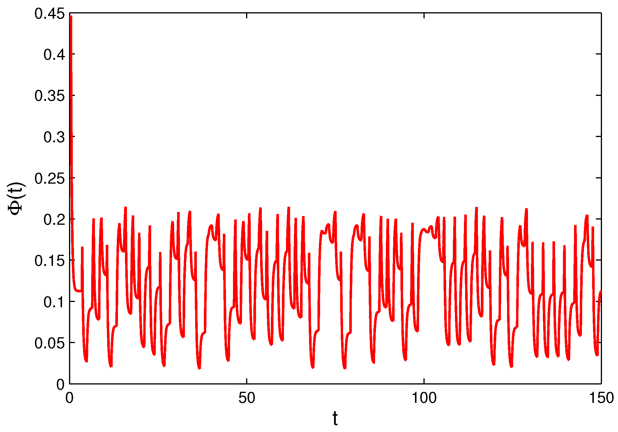
Example 1.

Consider the following discrete logistic map given by:

$$\begin{array}{c}\hfill {\chi }_{i+1}=\mu {\chi }_i(1-{\chi }_i),\end{array}$$

(13)

where $i\in \mathbb{Z}.$ We know that if $\mu \in (0,4]$, then the iterations of this map belong to the interval $[0,1]$ [54]. Moreover, if $\mu \in [3+{\left(\frac{2}{3}\right)}^{1/2},4]$, Equation (13) has an unpredictable solution. Let ${\Psi }_i,$ $i\in \mathbb{Z},$ denote an unpredictable solution of (13) for $\mu =3.93$. There exist a positive number ${\epsilon }_0$ and sequences $p_n{q}_n$ that diverge to infinity such that $|{\Psi }_{i+p_n}-{\Psi }_i|\to 0$ as $n\to \infty$ for each i in bounded intervals of integers and $|{\Psi }_{p_n+q_n}-{\Psi }_{q_n}|\ge {\epsilon }_0$ for each $n\in \mathbb{N}.$

Consider the following integral defined by:

$${\displaystyle \Theta \left(t\right)={\int }_{-\infty }^t{e}^{-4(t-s)}\Omega \left(s\right)ds,t\in \mathbb{R},}$$

where $\Omega \left(t\right)={\Psi }_i$ for $t\in [i,i+1),$ $i\in \mathbb{Z}.$ It is worth noting that $\Theta \left(t\right)$ is bounded on the whole real axis such that $\underset{t\in \mathbb{R}}{sup}\left|\Theta \left(t\right)\right|\le 1/4.$ In [37], it was proven that the function $\Theta \left(t\right)$ is an unpredictable function.

Since we do not know the initial value of the function $\Theta \left(t\right)$, we are not able to visualize it. For this reason, we represent the function $\Theta \left(t\right)$ as follows:

$${\displaystyle \Theta \left(t\right)={\int }_{-\infty }^t{e}^{-4(t-s)}\Omega \left(s\right)ds=e^{-4t}{\Theta }_0+{\int }_0^t{e}^{-4(t-s)}\Omega \left(s\right)ds,}$$

(14)

where ${\displaystyle {\Theta }_0={\int }_{-\infty }^0{e}^{4s}\Omega \left(s\right)ds}$. It is worth noting that the simulation of an unpredictable function is impossible, since the initial value is not known.

That is why, we simulate a function $\Phi \left(t\right)$ that approaches the function $\Theta \left(t\right)$ as time increases. Let us determine:

$${\displaystyle \Phi \left(t\right)=e^{-4t}{\Phi }_0+{\int }_0^t{e}^{-4(t-s)}\Omega \left(s\right)ds,}$$

(15)

where ${\Phi }_0$ is a fixed number, which is not necessarily equal to ${\Theta }_0$. Subtract equality (15) from equality (14) to obtain that $\Theta \left(t\right)-\Phi \left(t\right)=e^{-4t}({\Theta }_0-{\Phi }_0)$, $t\ge 0$. The last equation demonstrates that the difference $\Theta \left(t\right)-\Phi \left(t\right)$ exponentially diminishes. This means that the function $\Phi \left(t\right)$ exponentially tends to the unpredictable function $\Theta \left(t\right)$, i.e., the graphs of these functions approach, as time increases.

The functions $\Phi \left(t\right)$ and $\Theta \left(t\right)$ are the solutions of the differential equation:

$${\Phi }^{\prime }\left(t\right)=-4\Phi \left(t\right)+\Omega \left(t\right),$$

and instead of the curve describing the unpredictable solution $\Theta \left(t\right)$, we can take the graph of $\Phi \left(t\right)$, which approximates the first one asymptotically. In Figure 2, we depict the graph defined by the initial value $\Phi \left(0\right)=0.45$.

Example 2.

Consider the following Hopfield-type neural network given by:

$$\begin{array}{c}\hfill {\displaystyle x_i^{\prime }\left(t\right)=-a_i{x}_i\left(t\right)+\sum _{j=1}^3{b}_{ij}{f}_j\left(x_j\left(t\right)\right)+\sum _{j=1}^3{c}_{ij}{g}_j\left(x_j\left(\gamma \left(t\right)\right)\right)+{\vartheta }_i\left(t\right),}\end{array}$$

(16)

where $a_1=0.5,a_2=0.2,a_3=0.25,f_i\left(x_i\left(t\right)\right)=0.1tanh(x_i\left(t\right)/8)$, $g_i\left(x_i\left(t\right)\right)=0.05tanh(x_i\left(t\right)/6),$ $i=1,2,3$,

$$\left(\begin{array}{ccc}{b}_{11}& b_{12}& b_{13}\\ b_{21}& b_{22}& b_{23}\\ b_{31}& b_{32}& b_{33}\end{array}\right)=\left(\begin{array}{ccc}0.1& 0.2& 0.5\\ 0.3& 0.1& 0.2\\ 0.2& 0.1& 0.3\end{array}\right),\left(\begin{array}{ccc}{c}_{11}& c_{12}& c_{13}\\ c_{21}& c_{22}& c_{23}\\ c_{31}& c_{32}& c_{33}\end{array}\right)=\left(\begin{array}{ccc}0.1& 0.2& 0.1\\ 0.2& 0.2& 0.2\\ 0.1& 0.3& 0.1\end{array}\right)$$

and the time-varying stimulus is:

$$\left(\begin{array}{c}{\vartheta }_1\left(t\right)\\ {\vartheta }_2\left(t\right)\\ {\vartheta }_3\left(t\right)\end{array}\right)=\left(\begin{array}{c}-24\Theta \left(t\right)-0.04\\ 48{\Theta }^3\left(t\right)+0.05\\ 58{\Theta }^3\left(t\right)+0.03\end{array}\right).$$

Here, $\Theta \left(t\right)$ is the unpredictable function mentioned in Example 1.

Let the argument function $\gamma \left(t\right)={\xi }_k$ be defined by the sequences ${\theta }_k=k$, ${\xi }_k=\frac{2k+1}{2}+{\Psi }_k,k\in \mathbb{Z}.$

We can see that the conditions (C1)–(C8) are valid for the neural network (16) with $\lambda =0.2,\overline{\lambda }=0.5,$ $L_j=0.0125,{\overline{L}}_j=0.0083,$ $m_f=0.1,m_g=0.05,$ for $j=1,2,3$, and moreover, $m_v=6.04$, $K=1.1648$. If we accept $H=31$, then the system (16) satisfies all conditions of Theorem 1. Therefore, (16) has a unique exponentially stable unpredictable solution $x\left(t\right).$

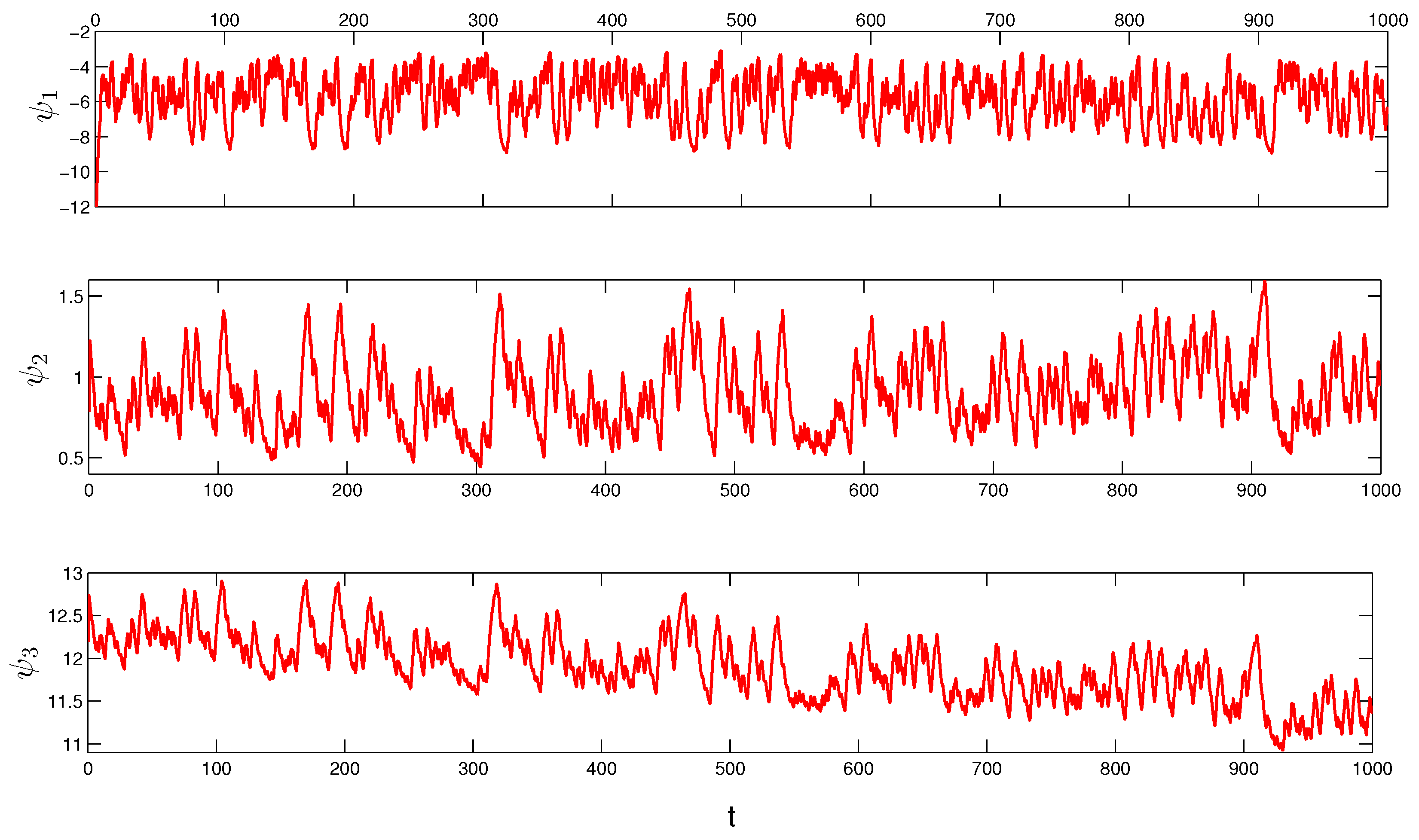
Since the initial value is not known precisely, it is not possible to simulate the unpredictable solution $x\left(t\right)$. For this reason, we consider another solution $\psi \left(t\right)=({\psi }_1\left(t\right),{\psi }_2\left(t\right),{\psi }_3\left(t\right))$, which starts initially at the point $\psi \left(0\right)=(-12.4956,0.7828,12.1987)$.

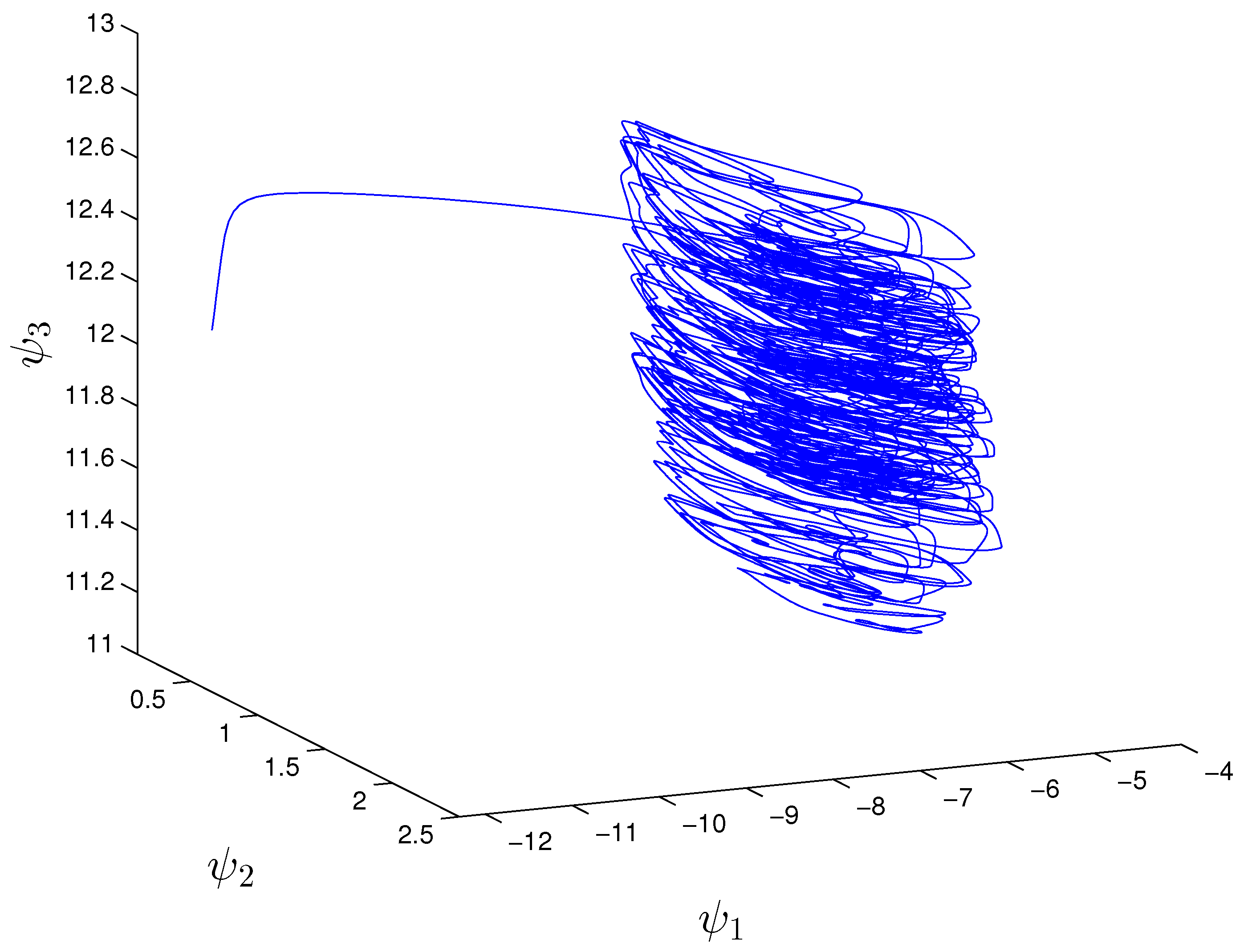
The graph of function $\psi \left(t\right)$ approaches the unpredictable solution $x\left(t\right)$ of Equation (16), as time increases. That is, instead of the curve describing the unpredictable solution, one can consider the graph of $x\left(t\right)$. We present the coordinates of the solution $\psi \left(t\right)$ in Figure 3. Moreover, Figure 4 indicates the trajectory of the solution.

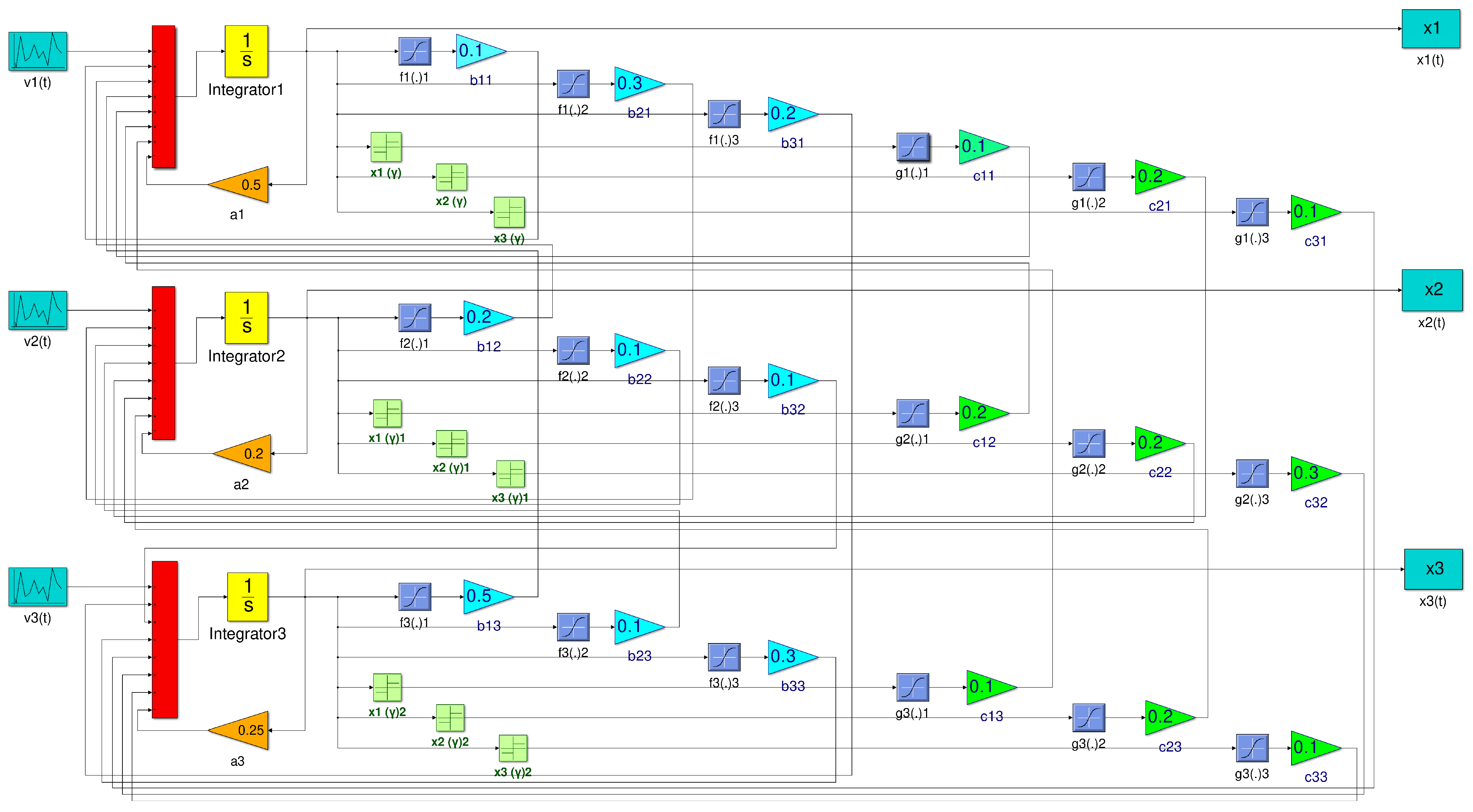
Further, we describe a circuit implementation of the proposed Hopfield-type neural network (16) using MATLAB Simulink. The Simulink model of the Hopfield-type neural network is depicted in Figure 5, and the symbols are described in

Table 2. Characteristics of elements of the block diagram in Figure 5.

Symbols	Description
	Integrator block
	Sum block
	Gain blocks with the values $a_i,b_{ij},c_{ij},i,j=1,2,3$
	Transfer function block, with nonlinear functions f and g
	MATLAB function block, with the piecewise constant function $\gamma \left(t\right)$
	Input function
	Output function

.

In the block diagram, we took the hyperbolic tangent transfer function as the sigmoid functions f and g. To implement the block diagram, we used the transfer function “tansig” from the MATLAB Simulink library. Inputs ${\vartheta }_1\left(t\right),{\vartheta }_2\left(t\right),{\vartheta }_3\left(t\right)$ are unpredictable functions.

References

- Akhmet, M. Principles of Discontinuous Dynamical Systems; Springer: New York, NY, USA, 2010. [Google Scholar]
- Wiener, J. Generalized Solutions of Functional Differential Equations; World Scientific: Singapore, 1993. [Google Scholar]
- Lakshmikantham, V.; Bainov, D.D.; Simeonov, P.S. Theory of Impulsive Differential Equations; World Scientific: Singapore, 1989. [Google Scholar]
- Gopalsamy, K. Stability and Oscillation in Delay Differential Equations of Population Dynamics; Kluwer Academic Publishers: Dordrecht, The Netherlands, 1992. [Google Scholar]
- Pinto, M. Asymptotic equivalence of nonlinear and quasi linear differential equations with piecewise constant arguments. Math. Comput. Model. 2009, 49, 1750–1758. [Google Scholar] [CrossRef]
- Coronel, A.; Maulén, C.; Pinto, M.; Sepúlveda, D. Dichotomies and asymptotic equivalence in alternately advanced and delayed differential systems. J. Math. Anal. Appl. 2017, 450, 1434–1458. [Google Scholar] [CrossRef] [Green Version]
- Huang, Z.; Wang, X.; Xia, Y. A topological approach to the existence of solutions for nonlinear differential equations with piecewise constant argument. Chaos Solitons Fractals 2009, 39, 1121–1131. [Google Scholar] [CrossRef]
- Akhmet, M.U. Stability of differential equations with piecewise constant arguments of generalized type. Nonlinear Anal. 2008, 68, 794–803. [Google Scholar] [CrossRef]
- Akhmet, M.U.; Aruğaslan, D. Lyapunov-Razumikhin method for differential equations with piecewise constant argument. Discret. Contin. Dyn. Syst. 2009, 25, 457–466. [Google Scholar] [CrossRef]
- Akhmet, M. Nonlinear Hybrid Continuous/Discrete-Time Models; Atlantis Press: Paris, France, 2011. [Google Scholar]
- Gopalsamy, K. Stability of artificial neural networks with impulses. Appl. Math. Comput. 2004, 154, 783–813. [Google Scholar] [CrossRef]
- Guan, Z.; Chen, G. On delayed impulsive Hopfield neural networks(1). Neural Netw. Off. J. Int. Neural Netw. Soc. 1999, 12, 273–280. [Google Scholar] [CrossRef]
- Xu, D.; Yang, Z. Impulsive delay differential inequality and stability of neural networks. J. Math. Anal. Appl. 2005, 305, 107–120. [Google Scholar] [CrossRef] [Green Version]
- Mohammad, S. Exponential stability in Hopfield-type neural networks with impulses. Chaos Solitons Fractals 2007, 32, 456–467. [Google Scholar] [CrossRef]
- Li, Y.; Lu, L. Global exponential stability and existence of periodic solution of Hopfield-type neural networks with impulses. Phys. Lett. A 2004, 333, 62–71. [Google Scholar] [CrossRef]
- Akhmet, M.; Yilmaz, E. Hopfield-type neural network system with piecewise constant argument. Int. J. Qual. Theory Differ. Equ. Appl. 2009, 3, 8–14. [Google Scholar] [CrossRef]
- Wan, L.; Wu, A. Stabilization control of generalized type neural networks with piecewise constant argument. J. Nonlinear Sci. Appl. 2016, 9, 3580–3599. [Google Scholar] [CrossRef] [Green Version]
- Pinto, M.; Sepúlveda, D.; Torres, R. Exponential periodic attractor of impulsive Hopfield-type neural network system with piecewise constant argument. Electron. J. Qual. Theory Differ. Equ. 2018, 34, 1–28. [Google Scholar] [CrossRef]
- Akhmet, M.; Yilmaz, E. Impulsive Hopfield-type neural network system with piecewise constant argument. Nonlinear Anal. Real World Appl. 2010, 11, 2584–2593. [Google Scholar] [CrossRef]
- Pajares, G. A Hopfield Neural Network for Image Change Detection. IEEE Trans. Neural Netw. 2006, 17, 1250–1264. [Google Scholar] [CrossRef] [PubMed]
- Ramya, C.; Kavitha, G.; Shreedhara, K.S. Recalling of images using Hopfield neural network model. arXiv 2011, arXiv:1105.0332. [Google Scholar]
- Soni, N.; Sharma, E.K.; Kapoor, A. Application of Hopfield neural network for facial image recognition. IJRTE 2019, 8, 3101–3105. [Google Scholar]
- Akhmet, M.U.; Enes, Y. Neural Networks with Discontinuous/Impact Activations; Springer: New York, NY, USA, 2014. [Google Scholar]
- Akhmet, M.; Aruğaslan, D.; Cengiz, N. Exponential stability of periodic solutions of recurrent neural networks with functional dependence on piecewise constant argument. Turk. J. Math. 2018, 42, 272–292. [Google Scholar] [CrossRef]
- Akhmet, M.U. Integral manifolds of differential equations with piecewise constant argument of generalized type. Nonlinear Anal. 2007, 66, 367–383. [Google Scholar] [CrossRef] [Green Version]
- Chiu, K.S.; Pinto, M.; Jeng, J. Existence and global convergence of periodic solutions in recurrent neural network models with a general piecewise alternately advanced and retarded argument. Acta Appl. Math. 2014, 133, 133–152. [Google Scholar] [CrossRef]
- Torres, R.; Pinto, M.; Castillo, S.; Kostić, M. Uniform Approximation of Impulsive Hopfield Cellular Neural Networks by Piecewise Constant Arguments on [τ,∞). Acta Appl. Math. 2021, 171, 8. [Google Scholar] [CrossRef]
- Akhmet, M.U. On the reduction principle for differential equations with piecewise constant argument of generalized type. J. Math. Anal. Appl. 2007, 336, 646–663. [Google Scholar] [CrossRef]
- Akhmet, M.; Fen, M.O. Poincaré chaos and unpredictable functions. Commun. Nonlinear Sci. Numer. Simulat. 2017, 48, 85–94. [Google Scholar] [CrossRef] [Green Version]
- Akhmet, M.; Fen, M.O. Unpredictable points and chaos. Commun. Nonlinear Sci. Numer. Simulat. 2016, 40, 1–5. [Google Scholar] [CrossRef] [Green Version]
- Akhmet, M.; Fen, M.O. Existence of unpredictable solutions and chaos. Turk. J. Math. 2017, 41, 254–266. [Google Scholar] [CrossRef]
- Akhmet, M.; Fen, M.O. Non-autonomous equations with unpredictable solutions. Commun. Nonlinear Sci. Numer. Simulat. 2018, 59, 657–670. [Google Scholar] [CrossRef]
- Akhmet, M.; Fen, M.O.; Tleubergenova, M.; Zhamanshin, A. Unpredictable solutions of linear differential and discrete equations. Turk. J. Math. 2019, 43, 2377–2389. [Google Scholar] [CrossRef]
- Akhmet, M.; Tleubergenova, M.; Zhamanshin, A. Quasilinear differential equations with strongly unpredictable solutions. Carpathian J. Math. 2020, 36, 341–349. [Google Scholar]
- Akhmet, M.U.; Fen, M.O.; Alejaily, E.M. Dynamics with Chaos and Fractals; Springer: Cham, Switzerland, 2020. [Google Scholar]
- Akhmet, M.; Tleubergenova, M.; Fen, M.O.; Nugayeva, Z. Unpredictable solutions of linear impulsive systems. Mathematics 2020, 8, 1798. [Google Scholar] [CrossRef]
- Akhmet, M.; Tleubergenova, M.; Nugayeva, Z. Strongly unpredictable oscillations of Hopfield-type neural networks. Mathematics 2020, 8, 1791. [Google Scholar] [CrossRef]
- Akhmet, M.; Seilova, R.; Tleubergenova, M.; Zhamanshin, A. Shunting inhibitory cellular neural networks with strongly unpredictable oscillations. Commun. Nonlinear Sci. Numer. Simulat. 2020, 89, 105287. [Google Scholar] [CrossRef]
- Akhmet, M.; Tleubergenova, M.; Zhamanshin, A. Inertial neural networks with unpredictable oscillations. Mathematics 2020, 8, 1797. [Google Scholar] [CrossRef]
- Miller, A. Unpredictable points and stronger versions of Ruelle–Takens and Auslander–Yorke chaos. Topol. Appl. 2019, 253, 7–16. [Google Scholar] [CrossRef]
- Thakur, R.; Das, R. Strongly Ruelle-Takens, strongly Auslander-Yorke and Poincaré chaos on semiflows. Commun. Nonlinear. Sci. Numer. Simulat. 2019, 81, 105018. [Google Scholar] [CrossRef]
- Akhmet, M.U. Almost Periodicity, Chaos, and Asymptotic Equivalence; Springer: New York, NY, USA, 2020. [Google Scholar]
- Yu, T.; Cao, D.; Liu, S.; Chen, H. Stability analysis of neural networks with periodic coefficients and piecewise constant arguments. J. Frankl. Inst. 2016, 353, 409–425. [Google Scholar] [CrossRef]
- Xi, Q. Global exponential stability of Cohen-Grossberg neural networks with piecewise constant argument of generalized type and impulses. Neural Comput. 2016, 28, 229–255. [Google Scholar] [CrossRef] [PubMed]
- Danciu, D. Qualitative behavior of the time delay Hopfield type neural networks with time varying stimulus. Ann. Univ. Craiova Ser. El. Eng. 2002, 26, 72–82. [Google Scholar]
- Guevara, M.R.; Glass, L.; Mackey, M.C.; Shrier, A. Chaos in neurobiology. IEEE Trans. Syst. Man Cybern. 1983, 13, 790–798. [Google Scholar] [CrossRef]
- Derrida, B.; Meir, R. Chaotic behavior of a layered neural network. Phys. Rev. A 1988, 38, 3116–3119. [Google Scholar] [CrossRef]
- Wang, L.; Pichler, E.E.; Ross, J. Oscillations and chaos in neural networks: An exactly solvable model. Proc. Nat. Acad. Sci. USA 1990, 87, 9467–9471. [Google Scholar] [CrossRef] [PubMed] [Green Version]
- Landau, I.D.; Sompolinsky, H. Coherent chaos in a recurrent neural network with structured connectivity. PLoS Comput. Biol. 2018, 14, e1006309. [Google Scholar] [CrossRef] [PubMed] [Green Version]
- Qu, J.; Wang, R.; Yan, C.; Du, Y. Oscillations and synchrony in a cortical neural network. Cogn. Neurodyn. 2014, 8, 157–166. [Google Scholar] [CrossRef] [PubMed]
- Muscinelli, S.P.; Gerstner, W.; Schwalger, T. How single neuron properties shape chaotic dynamics and signal transmission in random neural networks. PLoS Comput. Biol. 2019, 15, e1007122. [Google Scholar] [CrossRef]
- Penn, Y.; Segal, M.; Moses, E. Network synchronization in hippocampal neurons. Proc. Natl. Acad. Sci. USA 2016, 113, 3341–3346. [Google Scholar] [CrossRef] [PubMed] [Green Version]
- Bel, A.; Rotstein, H.G. Membrane potential resonance in non-oscillatory neurons interacts with synaptic connectivity to produce network oscillations. J. Comput. Neurosci. 2019, 46, 169–195. [Google Scholar] [CrossRef] [PubMed]
- Hale, J.; Koçak, H. Dynamics and Bifurcations; Springer: New York, NY, USA, 1991. [Google Scholar]