Stieltjes and Hamburger Reduced Moment Problem When MaxEnt Solution Does Not Exist

Abstract

For a given set of moments whose predetermined values represent the available information, we consider the case where the Maximum Entropy (MaxEnt) solutions for Stieltjes and Hamburger reduced moment problems do not exist. Genuinely relying upon MaxEnt rationale we find the distribution with largest entropy and we prove that this distribution gives the best approximation of the true but unknown underlying distribution. Despite the nice properties just listed, the suggested approximation suffers from some numerical drawbacks and we will discuss this aspect in detail in the paper.

1. Problem Formulation and MaxEnt Rationale

In the context of testable information that is, when a statement about a probability distribution whose truth or falsity is well-defined, the principle of maximum entropy states that the probability distribution which best represents the current state of knowledge is the one with largest entropy. In this spirit, Maximum Entropy (MaxEnt) methods are traditionally used to select a probability distribution in situations when some (prior) knowledge about the true probability distribution is available and several (up to an infinite set of) different probability distributions are consistent with it. In such a situation MaxEnt methods represent correct methods for doing inference about the true but unknown underlying distribution generating the data that have been observed.

Suppose that X be an absolutely continuous random variable having probability density function (pdf) f defined on an unbounded support ${\mathcal{S}}_X$ and that ${\left\{{\mu }_k^{\ast }\right\}}_{k=1}^M$, with ${\mu }_0^{\ast }=1$, be M finite integer moments whose values are pre-determined that is,

$${\mu }_k^{\ast }={\int }_{{\mathcal{S}}_X}{x}^{k}f\left(x\right)dx,k=0,\dots ,M,$$

(1)

for an arbitrary $M\in \mathbb{N}$. Quantities such as in (1) may be intended to represent the available (pre-determined) information relatively to X.

The Stieltjes (Hamburger) reduced moment problem [1] consists of recovering an unknown pdf f, having support ${\mathcal{S}}_X={\mathbb{R}}^{+}$ (${\mathcal{S}}_X=\mathbb{R}$), from the knowledge of prefixed moment set ${\left\{{\mu }_k^{\ast }\right\}}_{k=1}^M$.

Due to the non-uniqueness of the recovered density, the best choice among the (potentially, infinite) competitors may be done by invoking the Maximum Entropy (MaxEnt) principle [2] which consists in maximizing the Shannon-entropy

$$H_f=-{\int }_{{\mathcal{S}}_X}f\left(x\right)lnf\left(x\right)dx$$

under the constraints (1). Since entropy may be regarded as an objective measure of the uncertainty in a distribution, “... the MaxEnt distribution is uniquely determined as the one which is maximally non-committal with regard the missing information” ([2], p. 623) so that “...It agrees with is known but expresses maximum uncertainty with respect to all other matters, and thus leaves a maximum possible freedom for our final decisions to be influenced by the subsequent sample data” ([3], p. 231). In other words, the MaxEnt method dictates the most "reasonable and objective" distribution subject to given constraints.

More formally, in such situation we have to manage a constrained optimization problem involving Shannon entropy and a set of given constraints (here the first M integer moments and the normalization constraint given by (1) when $k=0$).

This problem is typically solved using the method of Lagrange multipliers leading to a MaxEnt distribution whose density function $f_M$ is given by [4], p. 59

$$f_{M\mid ({\mu }_1^{\ast },\dots ,{\mu }_M^{\ast })}\left(x\right)=exp\left(-\sum _{j=0}^M{\lambda }_j{x}^j\right),$$

(2)

fulfils the given constraints ${\left\{{\mu }_k^{\ast }\right\}}_{k=0}^M$ since

$${\mu }_k^{\ast }={\int }_{{\mathcal{S}}_X}{x}^k{f}_M\left(x\right)dx,k=0,1,...,M$$

(3)

and has entropy

$$H_{f_M}({\mu }_1^{\ast },\dots ,{\mu }_M^{\ast })=-{\int }_{{\mathcal{S}}_X}{f}_M\left(x\right)ln{f}_M\left(x\right)dx={\lambda }_0+\sum _{k=1}^M{\lambda }_j{\mu }_k^{\ast }$$

(4)

where

$$H_{f_M}({\mu }_1^{\ast },\dots ,{\mu }_M^{\ast })=\underset{f\in {\mathcal{C}}_M}{max}{H}_f({\mu }_1^{\ast },\dots ,{\mu }_M^{\ast })$$

and

$${\mathcal{C}}_M=:\left\{f\ge 0|{\int }_{{\mathcal{S}}_X}{x}^{k}f\left(x\right)dx={\mu }_k^{\ast },k=0,\dots ,M\right\}=\left\{f_{({\mu }_1^{\ast },\dots ,{\mu }_M^{\ast })}\right\}.$$

(5)

From now on, for sake of brevity, we will write each member f of ${\mathcal{C}}_M$ omitting the dependency on $({\mu }_1^{\ast },\dots ,{\mu }_M^{\ast })$, predetermined set of moments; hence, f and $f_M$ will stand for $f_{({\mu }_1^{\ast },\dots ,{\mu }_M^{\ast })}$ and $f_{M\mid ({\mu }_1^{\ast },\dots ,{\mu }_M^{\ast })}\in {\mathcal{C}}_M$, respectively. The same will be done for the corresponding entropies: we will write $H_f$ and $H_{f_M}$ in place of $H_f({\mu }_1^{\ast },\dots ,{\mu }_M^{\ast })$ and $H_{f_M}({\mu }_1^{\ast },\dots ,{\mu }_M^{\ast })$.

A few words about our notation are now opportune. Since in the sequel an arbitrary moment ${\mu }_j$ may play different roles, we establish to use

• ${\mu }_j^{\ast }$ for prescribed moments;
• ${\mu }_j$ for variable (free to vary) moments;
• ${\mu }_{j,f_{j-1}}$ for the j-th moment of $f_{j-1}$, that is ${\mu }_{j,f_{j-1}}={\int }_{{\mathcal{S}}_X}{x}^j{f}_{j-1}\left(x\right)dx$ (in general ${\mu }_j\ne {\mu }_j^{\ast }$)
• ${\mu }_j^{-}$ to indicate the smallest value of ${\mu }_j$, once $({\mu }_1^{\ast },\dots ,{\mu }_{j-1}^{\ast })$ are prescribed.

Our attention is solely addressed towards sequences ${\left\{{\mu }_k^{\ast }\right\}}_{k=1}^{\infty }$ whose underlying density f has finite entropy $H_f$. More precisely, only distributions with $H_f=-\infty$ are not considered. Indeed, once ${\left\{{\mu }_k^{\ast }\right\}}_{k=0}^{\infty }$ is assigned, $H_f=+\infty$ is not feasible, as it is well known in MaxEnt setup that $H_f\le H_{f_2}=\frac{1}{2}ln\left[2\pi e({\mu }_2^{\ast }-{\left({\mu }_1{}^{\ast }\right)}^2)\right]$ is finite because Lyapunov’s inequality ${\mu }_2^{\ast }-{\left({\mu }_1{}^{\ast }\right)}^2$ (Hamburger case) and $H_f\le H_{f_1}=1+ln{\mu }_1^{\ast }$ is finite for every ${\mu }_1^{\ast }>0$ (Stieltjes case).

Here $({\lambda }_0,\dots ,{\lambda }_M)$ is the vector of Lagrange multipliers, with ${\lambda }_M\ge 0$ to guarantee integrability of $f_M$. If it is possible to determine Lagrange multipliers from the constraints ${\left\{{\mu }_k^{\ast }\right\}}_{k=1}^M$ then the moment problem admits solution and $f_M$ is MaxEnt solution (which is unique in S due to strict concavity of (4)).

The above non negativity condition on ${\lambda }_M$ which is a consequence of unbounded support ${\mathcal{S}}_X$, is crucial and renders the moment problem solvable only under certain restrictive assumptions on the prescribed moment vector $({\mu }_1^{\ast },\dots ,{\mu }_M^{\ast })$. This is the ultimate reason upon which the present paper relies.

The existence conditions of the MaxEnt solution $f_M$ have been deeply investigated in literature ([5,6,7,8,9] just to mention some widely cited papers); over the years an intense debate—combining the results of the above papers—has established the correct existence conditions underlying the Stieltjes and Hamburger moment problem (more details on this topic may be found in the Appendix A).

On the other hand, when the existence conditions for $f_M$ are not satisfied, the non-existence of the MaxEnt solution in Stieltjes and Hamburger reduced moment problem poses a series of interesting and important questions about how to find an approximant of the unknown density f least committed to the information not given to us (still obeying to Jaynes’ Principle). This problem is addressed the present paper.

More formally, take ${\mathcal{C}}_M$ to be the set of the density functions satisfying the $M+1$ moment constraints (that is, they share the same $M+1$ predetermined moments) and let $\mu \left({\mathcal{C}}_M\right)$ be the moment space associated to ${\mathcal{C}}_M$; hence, the indeterminacy of the moment problem (1) follows.

A common way to regularize the problem, as recalled before, consists in applying the MaxEnt Principle obtaining ${\mathcal{E}}_M$, the set of MaxEnt densities functions which is a subset of ${\mathcal{C}}_M$; consequently, let $\mu \left({\mathcal{E}}_M\right)$ be the moment space relative to the set of MaxEnt densities functions ${\mathcal{E}}_M$. Because, in general, $\mu \left({\mathcal{C}}_M\right)$ strictly includes $\mu \left({\mathcal{E}}_M\right)$ there are admissible moment vectors in $\mathrm{Int}\left(\mu \left({\mathcal{C}}_M\right)\right)$, the interior of $\mu \left({\mathcal{C}}_M\right)$, for which the moment problem (1) is solvable but the MaxEnt problem (3) has no solution and the usual regularization based on MaxEnt strategy is therefore precluded.

The implications of such issue are often understated in practical applications where the usual procedure limits itself to:

• In the Stieltjes or symmetric Hamburger cases: to replace the support ${\mathbb{R}}^{+}$ ($\mathbb{R}$) with an arbitrarily large interval $[a,b]$. As a consequence of it, the problem is numerically solved within a proper interval $[a,b]$, changing the original Stieltjes (Hamburger) moment problem into Hausdorff one. In the MaxEnt setup, the latter admits a solution for each set ${\left\{{\mu }_k^{\ast }\right\}}_{k=1}^M\in \mathrm{Int}\left(\mu \left({\mathcal{C}}_M\right)\right)$ ([7], Theorem 2).
• If $f_M$ does not exist (conclusion drawn uniquely from numerical evidence), $f_{M-1}$ (Stieltjes case) or $f_{M-2}$ (symmetric Hamburger case) always exist (see Appendix A). In such a case, although the first M moments are known, we have to settle for a density constrained by ${\left\{{\mu }_k^{\ast }\right\}}_{k=1}^{M-1}$ or ${\left\{{\mu }_k^{\ast }\right\}}_{k=1}^{M-2}$. However, this is not completely coherent with the MaxEnt principle that prescribes to use not only the available but all the available information; hence discarding available information seems to be conceptually in contrast with the MaxEnt spirit. However, from the point of practical applications, to consider or not to consider the prefixed moment ${\mu }_M^{\ast }$ seems to have negligible effects on the summarizing quantities of the underlying distribution (mostly expected values of suitable functions) in which we may be interested in. We will resume this issue, after having carefully motivated and proved the proposed solution, in the last section of the paper devoted to discussion and conclusions.

We call the solutions 1. and 2. “forced” pseudo-solutions; they might indeed lead to the unpleasant fact that a MaxEnt solution always exists, although the original Stieltjes (Hamburger) moment problem does not admit any solution. Hence the crucial question is: does there exist a way to regularize the (indeterminate) moment problem (1) coherently with all and only the available information exploiting the MaxEnt rationale setup without forcing to unnatural solutions, i.e., based on totally inappropriate application of the MaxEnt principle?

Before proceed recall ${\mathcal{C}}_M$ and define the following class of density functions:

$${\tilde{\mathcal{C}}}_M=:\{f\ge 0|{\int }_S{x}^{k}f\left(x\right)dx={\mu }_k^{\ast },k=0,...,M,{\mu }_{M+1}=+\infty \}$$

(6)

with ${\tilde{\mathcal{C}}}_M\subset {\mathcal{C}}_M$, whose entries satisfy the given constraints expressed in terms of $M+1$ assigned integer moments ${\mu }_k^{\ast }=\mathbb{E}\left(X^k\right),k=0,1,\dots ,M$.

Now the question is: once ${\left\{{\mu }_k^{\ast }\right\}}_{k=1}^M\in \mu \left({\mathcal{C}}_M\right)\backslash \mu \left({\mathcal{E}}_M\right)$ are pre-determined (that is, the MaxEnt problem does not admit solution) what is the optimal choice of the pdf that we can select in place of $f_M$? Relying upon the MaxEnt rationale, the best substitute of the missing $f_M$ should be given by suitable one ${\tilde{f}}_M\in {\mathcal{C}}_M$ having the overall largest entropy; that is, select ${\tilde{f}}_M\in {\mathcal{C}}_M$ actually satisfying the relationship

$$\underset{f\in {\mathcal{C}}_M}{sup}{H}_f-H_{{\tilde{f}}_M}<\epsilon$$

(7)

for an arbitrarily small $\epsilon$.

We are aimed to find ${sup}_{f\in {\mathcal{C}}_M}{H}_f$, ${\tilde{f}}_M$ and the corresponding entropy $H_{{\tilde{f}}_M}$, proving that it may be accomplished by MaxEnt machinery (see Equations (9)–(11) below).

The remainder of the paper is organized as follows. Section 2 and Section 3 are devoted to evaluating the best pdf in Stieltjes and Hamburger cases respectively. We devote Section 4 to numerical aspects and in Section 5 we round up with some concluding remarks. In Appendix A. the existence conditions of MaxEnt distributions in Stieltjes and Hamburger case are shortly reviewed.

2. Stieltjes Case

Let us consider ${\left\{{\mu }_k^{\ast }\right\}}_{k=1}^M\in \mu \left({\mathcal{C}}_M\right)\backslash \mu \left({\mathcal{E}}_M\right)$; consequently $f_M$ does not exist. In this section we provide a formal justification about motivation (rationale) and optimality of the proposed substitute ${\tilde{f}}_M$ of the MaxEnt density $f_M$. We deal with the issue of selecting the "best” pdf both satisfying the constraints (given by predetermined integer moments) and with the overall largest entropy.

Before start, some relevant facts need to be collected together. Since MaxEnt density $f_M$ does not exist both $f_{M-1}$ with its M-th moment ${\mu }_{M,f_{M-1}}\le {\mu }_M^{\ast }$ and

$$f_{M+1}=f_{M+1}\left({\mu }_{M+1}\right)=f_{M+1\mid {\mu }_1^{\ast },\dots ,{\mu }_M^{\ast },{\mu }_{M+1}}\in {\mathcal{C}}_M$$

exist; the latter exists for any value ${\mu }_{M+1}>{\mu }_{M+1}^{-}$ (see Appendix A for more details).

Since the procedure here adopted remains valid for each value ${\mu }_M^{\ast }>{\mu }_{M,f_{M-1}}$, as ${\mu }_M^{\ast }\to +\infty$ from Lyapunov’s inequality, we have ${\mu }_{M+1}>{\left({\mu }_M^{\ast }\right)}^{\left(1+\frac{1}{M}\right)}$ and consequently ${\mu }_{M+1}\to +\infty$ too. As well, since MaxEnt density does not exist, some additional information not given to us must be added; of course, ${\mu }_{M+1}$ is the most suitable candidate to represent it.

Once this is established, the relevant question is: what value for ${\mu }_{M+1}$? Recalling that $H_{f_{M+1}}({\mu }_1^{\ast },\dots ,{\mu }_M^{\ast },{\mu }_{M+1})=H_{f_{M+1}}\left({\mu }_{M+1}\right)$ is monotonic increasing ([4], Equation (2.73), p. 59), with upper bound $H_{f_{M-1}}$ so that ${lim}_{{\mu }_{M+1}\to \infty }{H}_{f_{M+1}}\left({\mu }_{M+1}\right)$ exists, ${\mu }_{M+1}$ should assume the overall largest value, so that the decreasing of entropy is as small as possible.

Since ${\left\{{\mu }_k^{\ast }\right\}}_{k=1}^M\in \mu \left({\mathcal{C}}_M\right)\backslash \mu \left({\mathcal{E}}_M\right)$, $f_M$ and then $H_{f_M}$ are meaningless, ${\mathcal{C}}_M$ includes infinitely many f and ${sup}_{f\in {\mathcal{C}}_M}{H}_f$ must be calculated. The moment set $({\mu }_1^{\ast },\dots ,{\mu }_{M-1}^{\ast },{\mu }_M^{\ast }>{\mu }_{M,f_{M-1}},{\mu }_{M+1})$ is considered too, where ${\mu }_{M,f_{M-1}}$ is the M-th order moment of $f_{M-1}$ and ${\mu }_{M+1}$ varies continuously within $\mu \left({\mathcal{E}}_{M+1}\right)$ with

$$({\mu }_1^{\ast },\dots ,{\mu }_M^{\ast },{\mu }_{M+1}^{-})\in \partial \mu \left({\mathcal{C}}_{M+1}\right).$$

(8)

If $f_{M+1}\left({\mu }_{M+1}\right)$ is density corresponding to the set of moments (8), the following theorem holds.

Theorem 1.

The following two relationships hold

$$\underset{f\in {\mathcal{C}}_M}{sup}{H}_f=H_{f_{M-1}}$$

(9)

and

$$\underset{{\mu }_{M+1}\to \infty }{lim}{H}_{f_{M+1}}\left({\mu }_{M+1}\right)=H_{f_{M-1}}.$$

(10)

Now, ${\tilde{f}}_M$ is identified with $f_{M+1}\left({\tilde{\mu }}_{M+1}\right)$ where ${\tilde{\mu }}_{M+1}$ is such that

$$H_{f_{M-1}}-H_{f_{M+1}}\left({\tilde{\mu }}_{M+1}\right)<\epsilon$$

(11)

and ε indicates a fixed tolerance.

Proof. 

If $f_M$ does not exist, $f_{M-1}$ exists with entropy $H_{f_{M-1}}$ and M-th moment ${\mu }_{M,f_{M-1}}<{\mu }_M^{\ast }$ respectively. The function $H_{f_M}\left({\mu }_M\right)$, with ${\mu }_M>{\mu }_M^{-}$, is monotonic increasing. As

• ${\mu }_M^{\ast }\le {\mu }_{M,f_{M-1}}$ one has ${sup}_{f\in {\mathcal{C}}_M}{H}_f={max}_{f\in {\mathcal{C}}_M}{H}_f=H_{f_M}\le H_{f_{M-1}}$. The latter represents the maximum attainable entropy once $({\mu }_1^{\ast },\dots ,{\mu }_M^{\ast })$ are prescribed;
• ${\mu }_M^{\ast }>{\mu }_{M,f_{M-1}}$, from monotonicity of $H_{f_M}\left({\mu }_M\right)$ it follows ${sup}_{f\in {\mathcal{C}}_M}{H}_f=H_{f_{M-1}}$ independent on ${\mu }_M^{\ast }$. Equivalently, $H_{f_{M-1}}$ is strict upper bound for the entropies of all densities which have same lower moments $({\mu }_1^{\ast },...,{\mu }_{M-1}^{\ast })$ as $f_{M-1}$ but whose highest moment ${\mu }_M^{\ast }$ exceeds ${\mu }_{M,f_{M-1}}$.

Hence Equation (9) is proved.

Let us now consider the suitable class

$${\mathcal{E}}_{M+1}\left({\mu }_{M+1}\right)=\left\{f_{M+1}\left({\mu }_{M+1}\right)=f_{M+1\mid {\mu }_1^{\ast },\dots ,{\mu }_M^{\ast },{\mu }_{M+1}}\left(x\right)\right\}$$

(12)

where ${\mu }_{M+1}\in ({\mu }_{M+1}^{-},\infty )$ is assumed as parameter and ${\mu }_{M,f_{M-1}}$ is the M-th order moment of $f_{M-1}$. Equivalently, the entries of ${\mathcal{E}}_{M+1}\left({\mu }_{M+1}\right)$ are MaxEnt pdfs constrained by $({\mu }_1^{\ast },...,{\mu }_M^{\ast },{\mu }_{M+1})$, belong to ${\mathcal{C}}_M$ and, primarily, they all have analytically tractable entropy.

In (5), (6) and (12) three classes of functions ${\mathcal{C}}_M$, ${\tilde{\mathcal{C}}}_M$ and ${\mathcal{E}}_{M+1}\left({\mu }_{M+1}\right)$ had been defined. Relying upon the identity ${\mathcal{C}}_M={\mathcal{E}}_{M+1}\left({\mu }_{M+1}\right)\cup ({\mathcal{C}}_M\backslash {\mathcal{E}}_{M+1}\left({\mu }_{M+1}\right)\backslash {\tilde{\mathcal{C}}}_M)\cup {\tilde{\mathcal{C}}}_M$ we investigate the entropy $H_f$ of functions f belonging to (a) ${\mathcal{E}}_{M+1}\left({\mu }_{M+1}\right)$, (b) ${\mathcal{C}}_M\backslash {\mathcal{E}}_{M+1}\left({\mu }_{M+1}\right)\backslash {\tilde{\mathcal{C}}}_M$ and (c) ${\tilde{\mathcal{C}}}_M$ respectively.

• Consider that $H_{f_{M+1}}\left({\mu }_{M+1}\right)$, bounded by $H_{f_{M-1}}$ from above, is a differentiable monotonic increasing function of ${\mu }_{M+1}$ and then it tends to a finite limit so that

  $$\underset{f_{M+1\mid {\mu }_{M+1}\in {\mathcal{E}}_{M+1}\left({\mu }_{M+1}\right)}}{sup}{H}_{f_{M+1}}\left({\mu }_{M+1}\right)=\underset{{\mu }_{M+1}\to \infty }{lim}{H}_{f_{M+1}}\left({\mu }_{M+1}\right).$$
• Each $f\in {\mathcal{C}}_M\backslash {\mathcal{E}}_{M+1}\left({\mu }_{M+1}\right)\backslash {\tilde{\mathcal{C}}}_M$ has entropy $H_f$ and its $(M+1)$-th finite moment, say ${\mu }_{M+1,f}$. Since f and $f_{M+1\mid {\mu }_{M+1,f}}$ share same moments $({\mu }_1^{\ast },...,{\mu }_M^{\ast },{\mu }_{M+1,f})$ then $H_f\le H_{f_{M+1}}\left({\mu }_{M+1,f}\right)$ holds, from which

  $$\underset{f\in ({\mathcal{C}}_M\backslash {\mathcal{E}}_{M+1}\left({\mu }_{M+1}\right)\backslash {\tilde{\mathcal{C}}}_M)}{sup}{H}_f\le \underset{f_{M+1\mid {\mu }_{M+1}\in {\mathcal{E}}_{M+1}\left({\mu }_{M+1}\right)}}{sup}{H}_{f_{M+1}}\left({\mu }_{M+1}\right)=\underset{{\mu }_{M+1}\to \infty }{lim}{H}_{f_{M+1}}\left({\mu }_{M+1}\right).$$
• In analogy with (12), let us introduce the following class

  $${\mathcal{C}}_{M+1}\left({\mu }_{M+1}\right)=\left\{f\left({\mu }_{M+1}\right)=f_{\mid {\mu }_1^{\ast },\dots ,{\mu }_M^{\ast },{\mu }_{M+1}}\left(x\right)\right\}$$

  where ${\mu }_{M+1}>{\mu }_{M+1}^{-}$ assumes arbitrary values. For a fixed ${\mu }_{M+1}$, each $f\in {\mathcal{C}}_{M+1}\left({\mu }_{M+1}\right)$ satisfies the following inequality

  $$H_f\le \underset{f\in {\mathcal{C}}_{M+1}\left({\mu }_{M+1}\right)}{sup}{H}_f=H_{f_{M+1}}\left({\mu }_{M+1}\right).$$
  Taking ${\mu }_{M+1}\to \infty$, ${\mathcal{C}}_{M+1}\left({\mu }_{M+1}\right)$ coincides with ${\tilde{\mathcal{C}}}_M$ and then

  $$\underset{f\in {\tilde{\mathcal{C}}}_M}{sup}{H}_f=\underset{{\mu }_{M+1}\to \infty }{lim}{H}_{f_{M+1}}\left({\mu }_{M+1}\right).$$

Collecting together both the achieved results in above items (a), (b), (c) and taking into account (9) one has

$$\underset{f\in {\mathcal{C}}_M}{sup}{H}_f=\underset{{\mu }_{M+1}\to \infty }{lim}{H}_{f_{M+1}}\left({\mu }_{M+1}\right)=H_{f_{M-1}}.$$

Hence Equation (10) is also proved.

Equation (10) is restated as follows: if $\epsilon$ indicates a fixed tolerance, there exists a value ${\tilde{\mu }}_{M+1}$ of ${\mu }_{M+1}$ such that $H_{f_{M-1}}-H_{f_{M+1}}\left({\tilde{\mu }}_{M+1}\right)<\epsilon$ holds. Next ${\tilde{f}}_M$ is identified with $f_{M+1}\left({\tilde{\mu }}_{M+1}\right)$ so that its entropy $H_{{\tilde{f}}_M}$ coincides with $H_{f_{M+1}}\left({\tilde{\mu }}_{M+1}\right)$. From which the wanted result $H_{f_{M-1}}-H_{{\tilde{f}}_M}<\epsilon$ (or, equivalently (7)) follows. As a consequence ${\tilde{f}}_M$ is the proposed substitute of $f_M$ and Equation (11) is proved. □

In conclusion:

• As $f_M$ does not exist, although the current use of MaxEnt fails, a solution is found back to (9)–(11) from which the desired result (7).
• The existence of MaxEnt $f_M$ implies its uniqueness, unlike ${\tilde{f}}_M$ which depends on the assumed tolerance. In numerical Examples below just above remark will be actually used.

3. Hamburger Case

The non-symmetric Hamburger case when M even is here disregarded because the existence of the MaxEnt solution $f_M$ is guaranteed. Now, we will concentrate our attention on the symmetric case with $M\ge 4$ and on the non-symmetric case with $M\ge 3$ odd. In both cases, thanks to MaxEnt formalism, the procedure used in Stieltjes case can be extended to Hamburger one (see [9]); this fact represents one of the main advantages of MaxEnt machinery.

3.1. Symmetric Case with $M\ge 4$ Even

We recall $f_M$ is symmetric function for every M even so that Lagrange multipliers ${\lambda }_{2j-1}=0$.

Theorem 2.

Suppose the moment set $({\mu }_1^{\ast },...,{\mu }_M^{\ast })$ is prescribed and $f_M$ does not exist. Symmetric Hamburger case is analogous to Stieltjes one and then Theorem 1 holds true, with ${\mu }_{M+1}$ replaced by ${\mu }_{M+2}$ and ${\mu }_{M-1}$ by ${\mu }_{M-2}$.

Proof. 

Just remember that if $f_M$ does not exist for a prescribed moment set $({\mu }_1^{\ast },...,{\mu }_M^{\ast })$ then $f_{M-2}$ exists with its next moments ${\mu }_{M-1,f_{M-2}}$, ${\mu }_{M,f_{M-2}}$ and entropy $H_{f_{M-2}}$. If ${\mu }_M^{\ast }={\mu }_{M,f_{M-2}}$ holds, then $H_{f_{M-2}}$ is the maximum attainable entropy. In analogy with (12) let

$${\mathcal{E}}_{M+2}=\left\{f_{M+2}\left({\mu }_{M+2}\right)=:f_{M+2\mid ({\mu }_1^{\ast },\dots ,{\mu }_M^{\ast },{\mu }_{M+1}^{\ast }=0,{\mu }_{M+2}},{\mu }_{M+2}\in ({\mu }_{M+2}^{-},\infty )\right\}$$

where the parameter ${\mu }_{M+2}$ is introduced and thanks to MaxEnt machinery the proof continues analogously to the Stieltjes case. □

3.2. Non-Symmetric Case with $M\ge 3$ Odd

If M is odd $f_M$ does not exist for every set of moments belonging to $\mu \left({\mathcal{C}}_M\right)$ because ${\int }_{\mathbb{R}}{f}_M\left(x\right)dx=+\infty$. We now look at the problem from a different point of view. Suppose $({\mu }_1^{\ast },...,{\mu }_M^{\ast })\in \mu \left({\mathcal{C}}_M\right)$ is prescribed. In general $f_{M-1}$ exists (equivalently, $({\mu }_1^{\ast },...,{\mu }_{M-1}^{\ast })\in \mu \left({\mathcal{E}}_{M-1}\right)$ (see Appendix), with its M-th moment ${\mu }_{M,f_{M-1}}$. Two alternatives are possible:

• ${\mu }_M^{\ast }={\mu }_{M,f_{M-1}}$ then $f_M$ with ${\lambda }_M=0$ exists and coincides with $f_{M-1}$. Then usual MaxEnt method may be used;
• ${\mu }_M^{\ast }\ne {\mu }_{M,f_{M-1}}$ (highly probable case), then $f_M$ does not exist.

Both items 1. and 2. recall the Stieltjes case; more precisely, item (ii) may be solved taking into account $f_{M+1}\left({\mu }_{M+1}\right)\in {\mathcal{E}}_{M+1}$ (which exists for each ${\mu }_{M+1}>{\mu }_{M+1}^{-}$). Then non-symmetric case, with M odd and for every set of moments belonging to $\mu \left({\mathcal{C}}_M\right)$, is solved analogously to the Stieltjes case and Theorem 1 holds true. A consequence of achieved results in this section is the following. Let us consider a non symmetric Hamburger moment. In Theorem 1 we proved

$$H_{f_{M-1}}=\underset{f\in {\mathcal{C}}_M}{sup}{H}_f=\underset{{\mu }_{M+1}\to \infty }{lim}{H}_{f_{M+1}}\left({\mu }_{M+1}\right).$$

Since the entropy is monotonic non increasing as M increases, the latter equalities enable us to set $H_{f_M}=H_{f_{M-1}}$. As a consequence, the two subsequences $\left\{H_{f_{2M}}\right\}$ and $\left\{H_{f_{2M-1}}\right\}$ have coinciding entries. In past paper Milev and Tagliani proved that $\left\{H_{f_{2M}}\right\}$ converges to $H_f$ ([10], Theorem 1). Joining together the two achievements, both $\left\{H_{f_{2M}}\right\}$ and $\left\{H_{f_{2M-1}}\right\}$ converge to the same limit $H_f$, then so does $\left\{H_{f_M}\right\}$, filling the gaps left by even moments.

4. Numerical Aspects

The procedure just above described and rooted on MaxEnt machinery suffers from some numerical drawbacks which will be here discussed. It deserves to recall similar drawbacks had been previously found ([11,12]) although for the special value $M=4$ in Hamburger case, exploring special regions of the moment space. Essentially, numerical troubles arise because the expected solution $f_{M+1}$ is contaminated with a small wiggle that (a) moving to infinity, (b) is scaled in such a way that its contribution to the (M + 1)-th order moment ${\mu }_{M+1}$ is always $O\left(1\right)$ and (c) may become invisible to numerical methods of quadrature.

Now we provide some theoretical ground to justify above heuristics, which holds true in both Hamburger and Stieltjes case thanks to MaxEnt formalism. First of all, under the constraints $({\mu }_1^{\ast },\dots ,{\mu }_M^{\ast },{\mu }_{M+1})$, we prove the wiggle exists. At this purpose both the relationships ${\lambda }_M<0$ for each ${\mu }_{M+1}$ and ${\lambda }_{M+1}\to 0$ as ${\mu }_{M+1}\to \infty$ have to be proved.

• ${\lambda }_M<0$ for each ${\mu }_{M+1}$. From Appendix we recalled if $f_{M-1}$ exists with its M-th moment ${\mu }_{M,f_{M-1}}$, MaxEnt $f_M$ does not exist if ${\mu }_M^{\ast }>{\mu }_{M,f_{M-1}}$. Let us consider $f_M$ where ${\mu }_M$ varies continuously. Then ${\lambda }_M$ is monotonically decreasing ([9], Equation (2.1)) with ${\lambda }_M=0$ as ${\mu }_M={\mu }_{M,f_{M-1}}$. As a consequence no set $({\lambda }_1,...,{\lambda }_M)$ satisfies the constraints (${\mu }_1^{\ast },\dots ,{\mu }_M^{\ast }$ ) since the monotonicity of ${\lambda }_M$ would require ${\lambda }_M<0$. Let us consider $f_{M+1}$ where ${\mu }_{M+1}$ varies continuously. Here, for each ${\mu }_{M+1}$, ${\lambda }_{M+1}>0$ guarantees integrability, so that ${\lambda }_M$ may assume every real value. Collecting together the results about ${\lambda }_M$, the set $({\lambda }_1,\dots ,{\lambda }_{M-1},{\lambda }_M<0,{\lambda }_{M+1})$ satisfies the constraints $({\mu }_1^{\ast },\dots ,{\mu }_M^{\ast },{\mu }_{M+1})$ for each ${\mu }_{M+1}$. Equivalently, we can assert $({\lambda }_1,\dots ,{\lambda }_{M-1},{\lambda }_M<0)$ are appointed to meet $({\mu }_1^{\ast },\dots ,{\mu }_M^{\ast })$, whilst ${\lambda }_{M+1}$ to meet ${\mu }_{M+1}$.
• ${\lambda }_{M+1}\to 0$ as ${\mu }_{M+1}\to \infty$. Differentiating (4) with respect to ${\lambda }_{M+1}$ and recalling the relationship ([9], Equation (2.1))

  $$\sum _0^M{\mu }_j^{\ast }\frac{d{\lambda }_j}{d{\mu }_{M+1}}+{\mu }_{M+1}\frac{d{\lambda }_{M+1}}{d{\mu }_{M+1}}=0$$

  one has

  $$\frac{d{H}_{f_{M+1}}\left({\mu }_{M+1}\right)}{d{\mu }_{M+1}}=\sum _0^M{\mu }_j^{\ast }\frac{d{\lambda }_j}{d{\mu }_{M+1}}+{\mu }_{M+1}\frac{d{\lambda }_{M+1}}{d{\mu }_{M+1}}+{\lambda }_{M+1}={\lambda }_{M+1}.$$
  From Theorem 1 we proved, as ${\mu }_{M+1}\to \infty$, $H_{f_{M+1}}\to H_{f_{M-1}}$, so that $\frac{d{H}_{f_{M+1}\left({\mu }_{M+1}\right)}}{d{\mu }_{M+1}}\to 0$ and then ${\lambda }_{M+1}\to 0$ too.

We are ready to prove the statement concerning the fact that $f_{M+1}\left({\mu }_{M+1}\right)$ exhibits a small wiggle at $x\gg 1$ (analogously, in symmetric Hamburger case the wiggle is exhibited at $\mid x\mid \gg 1$). At $x\gg 1$

$$f_{M+1}\left(x\right)\sim exp\left(-{\lambda }_M{x}^M-{\lambda }_{M+1}{x}^{M+1}\right)$$

so that $f_{M+1}$ admits maximum value at

$$x_{\mathrm{wig}}=-\frac{M{\lambda }_M}{(M+1){\lambda }_{M+1}}>0.$$

As ${\mu }_{M+1}$ increases we proved the relationships ${\lambda }_M<0$ and ${\lambda }_{M+1}\to 0$, so that $x_{\mathrm{wig}}>0$ moves to infinity (from numerical evidence, as ${\mu }_{M+1}$ increases, $\mid {\lambda }_M\mid \to 0$ too much slower than ${\lambda }_{M+1}$). Since $f_{M+1}$ has finite moments $({\mu }_1^{\ast },...,{\mu }_M^{\ast })$ for each ${\mu }_{M+1}$, it follows the wiggle in a compact packet is scaled in such a way that its contribution to the (M + 1)-th order moment ${\mu }_{M+1}$ is always $O\left(1\right)$ (whilst for all higher moments the contribution due to this maximum obviously grows without bound, as a consequence of Lyapunov’s inequality).

An additional complication comes from the fact that height and position of wiggle is extremely sensitive to the parameters ${\lambda }_M$ and ${\lambda }_{M+1}$, so that it becomes progressively smaller and smaller until to be “invisible” if an unsuitable numerical method of quadrature is adopted. As a consequence the procedure becomes increasingly ill-conditioned to such a degree that numerical error precludes finding a suitable solution. As remedy, for instance, the quadrature on the unbounded domain has to be mapped onto finite interval, as well an adaptive quadrature is required. Since the wiggle moves along x-axis as ${\mu }_{M+1}$ increases, a fixed nodes quadrature formula could be unsuitable as the wiggle could become invisible for some values of ${\mu }_{M+1}$.

Above remedies are just a numerical trick, not a reduction of Stieltjes or Hamburger problem into Hausdorff one. Indeed, all the subsequent numerical examples consider and use random variables X having unbounded support ${\mathbb{R}}^{+}$ or $\mathbb{R}$.

As well the dual formulation, which evaluates $({\lambda }_1,...,{\lambda }_{M+1})$ minimizing the potential function

$${\left\{{\lambda }_j\right\}}_{j=1}^{M+1}:\underset{{\lambda }_1,...,{\lambda }_{M+1}}{min}[ln({\int }_{S}exp(-\sum _{j=1}^{M+1}{\lambda }_j{x}^j)dx)+\sum _{j=1}^M{\lambda }_j{\mu }_j^{\ast }+{\lambda }_{M+1}{\mu }_{M+1}]$$

avoids the computation of higher moments, as required by Newton-type methods by solving (3).

The drawbacks just illustrated lead us to equip the stopping criterion (7) based on entropy with a further one based on the moments, which allows us the relationship ${\mu }_{j,f_{M+1}}={\mu }_j^{\ast },j=1,...,M$ holds true. That is,

$$\underset{1\le j\le M}{max}\mid \frac{{\mu }_j^{\ast }-{\mu }_{j,f_{M+1}}}{{\mu }_j^{\ast }}\mid <{\epsilon }_1$$

(13)

(or involving the absolute error) for a proper ${\epsilon }_1$.

The following question arises: it is ${\tilde{f}}_M$, here identified with $f_{M+1}\left({\tilde{\mu }}_{M+1}\right)$ and ${\tilde{\mu }}_{M+1}$ is chosen so that stopping criteria (7) and (13) are verified, an acceptable approximation of underlying unknown density? Although the wiggle has non-physical meaning, nevertheless from the approximate density one like to calculate accurate and interesting quantities. We will resume the issue in the final part of the paper.

For practical purposes in both Stieltjes and Hamburger case ${\tilde{f}}_M$ is calculated according to (9)–(11) uniquely by means of MaxEnt machinery following these two distinct steps

• First, the sequence ${\left\{{\mu }_k^{\ast }\right\}}_{k=0}^M$ is prescribed and $f_M$ does not exists; then we know $f_{M-1}$ exists with entropy $H_{f_{M-1}}$;
• The next step relies upon on the monotonicity of $H_{f_{M+1}}\left({\mu }_{M+1}\right)$. If $\epsilon$ indicates a fixed tolerance, $f_{M+1}\left({\mu }_{M+1}\right)$ is calculated taking increasing values of ${\mu }_{M+1}$ until for some ${\tilde{\mu }}_{M+1}$ inequality $H_{f_{M-1}}-H_{f_{M+1}}\left({\tilde{\mu }}_{M+1}\right)<\epsilon$ is satisfied, assuming implicitly (13) is satisfied too. Next ${\tilde{f}}_M\equiv f_{M+1}\left({\tilde{\mu }}_{M+1}\right)$ is set.

Before to illustrate some numerical examples that confirm the goodness of the proposed method, it is worth spend some words discussing the outlined procedure. The calculation of ${\tilde{f}}_M$ is obtained through an approximate procedure and hence has a limited range of applicability. The main problem is the presence of wiggles; at the end to contain their detrimental effect it is necessary that convergence of $H_{f_{M+1}}\left({\mu }_{M+1}\right)$ to $H_{f_{M-1}}$ be fast. For example, the value ${\mu }_M^{\ast }$ that precludes the existence of $f_M$ in the Stieltjes case, must be such that the difference ${\mu }_M^{\ast }-{\mu }_{M,f_{M-1}}$ be small. Larger values make the convergence of $H_{f_{M+1}}\left({\mu }_{M+1}\right)$ to $H_{f_{M-1}}$ slow, allowing the generation of a small wiggle at great distance. The latter may become invisible to numerical quadrature methods.

Below are some numerical examples which both take into account the above remarks about the difference ${\mu }_M^{\ast }-{\mu }_{M,f_{M-1}}$ and illustrate the theoretical and numerical aspects mentioned above.

Example 1.

The Stieltjes case with $M=2$ and prescribed $({\mu }_1^{\ast },{\mu }_2^{\ast })$ is considered. Now $f_M$ exists if and only if the inequality ${\left({\mu }_1^{\ast }\right)}^2<{\mu }_2^{\ast }\le 2{\left({\mu }_1^{\ast }\right)}^2$ holds ([5], Theorem 2). The moment set $\{({\mu }_1,{\mu }_2)\mid {\mu }_2=2{\mu }_1^2\mid {\mu }_1>0\}\in Int\left(\mu \left({\mathcal{C}}_M\right)\right)$ represents an additional boundary in $\mu \left({\mathcal{C}}_M\right)$. If the moments satisfy the reverse inequality ${\mu }_2^{\ast }>2{\left({\mu }_1^{\ast }\right)}^2$ there is no pdf which maximizes the entropy.

We consider the latter case taking ${\mu }_1^{\ast }=1$ and ${\mu }_2^{\ast }=2.1$; then $f_{M+1}\left({\tilde{\mu }}_{M+1}\right)$ is calculated by means of (11), with $H_{f_{M-1}}=1+ln{\mu }_1^{\ast }=1$. Values of entropy $H_{f_{M+1}}\left({\mu }_{M+1}\right)$ with increasing values of ${\mu }_{M+1}>{\mu }_{M+1}^{-}=4.41$ not reported here lead to conclusion that the entropy stabilizes rapidly as ${\mu }_{M+1}$ increases. This may be an evidence of high accuracy in the reconstruction.

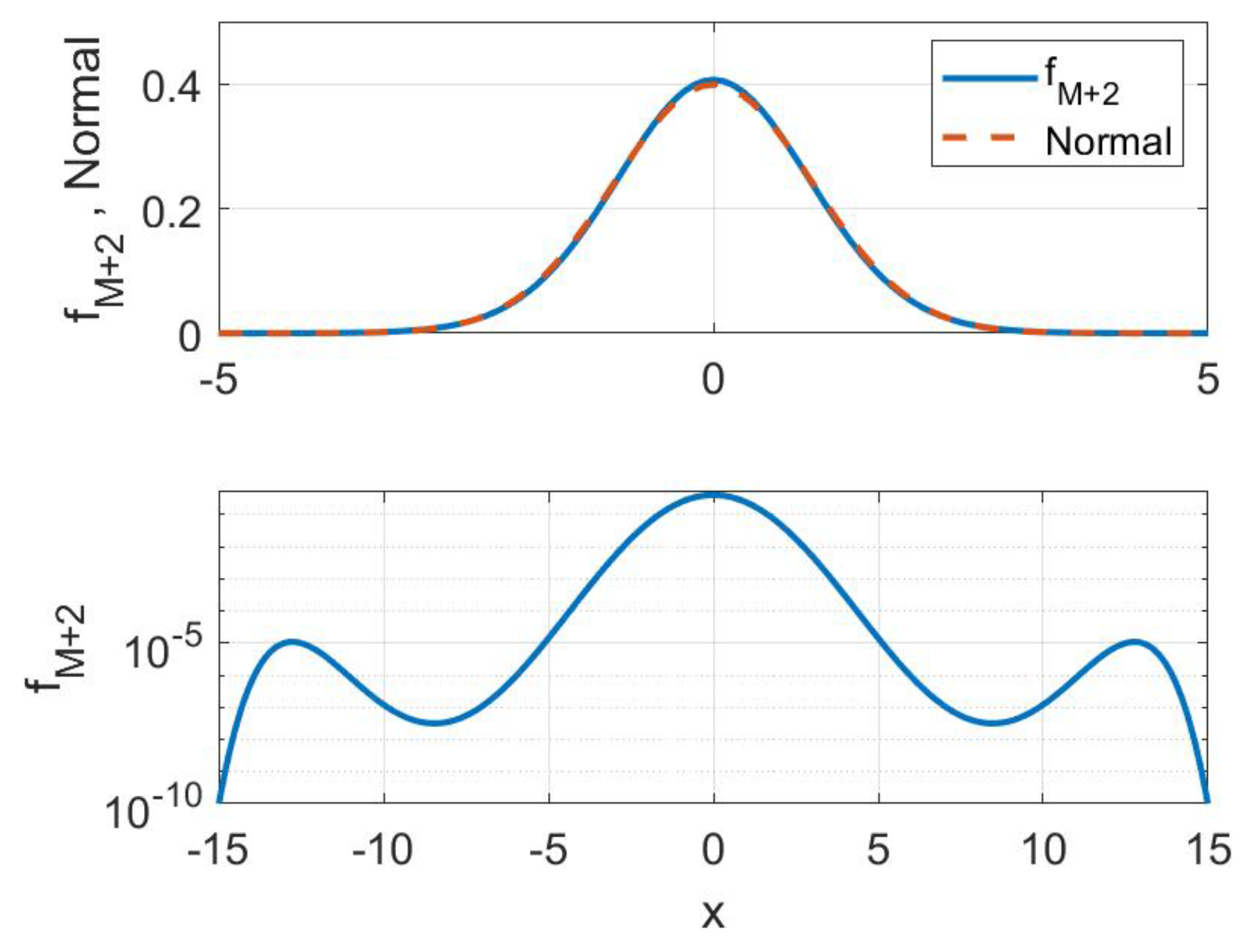
Taking $\epsilon ={10}^{-4}$, Equation (11) is satisfied starting from ${\tilde{\mu }}_{M+1}=20$. Then ${\tilde{f}}_M$, which is identified with $f_{M+1}\left({\tilde{\mu }}_{M+1}\right)$, jointly with $f_{M-1}$ are displayed in Figure 1 (top). The difference between ${\tilde{f}}_M$ and $f_{M-1}$ is insignificant since ${\mu }_M^{\ast }-{\mu }_{M,f_{M-1}}=0.1$ was chosen to avoid the dentrimental effect of wiggle. In Figure 1 (bottom) the same $f_{M+1}\left({\tilde{\mu }}_{M+1}\right)$, on a logarithmic scale and on extended x-axis scale, is reported to evidenciate the presence of small wiggle. The moments ${\mu }_{1,{\tilde{f}}_M}$, ${\mu }_{2,{\tilde{f}}_M}$ satisfy $\mid {\mu }_1^{\ast }-{\mu }_{1,{\tilde{f}}_M}\mid \sim {10}^{-8}$, $\mid {\mu }_2^{\ast }-{\mu }_{2,{\tilde{f}}_M}\mid \sim {10}^{-6}$, respectively. It can be concluded ${\tilde{f}}_M\equiv f_{M+1}\left({\tilde{\mu }}_{M+1}\right)$ satisfies all the expected theoretical properties and can be considered the "best" substitute of the missing $f_M$.

Example 2.

Hamburger case with $M=3$; here ${\mu }_1^{\ast }=0,{\mu }_2^{\ast }=1,{\mu }_3^{\ast }=0.5$, with the skewness = 0.5, are assumed. MaxEnt density $f_M$ does not exist if the first 3 moments are specified and the skewness is required to be non-zero. Then $f_M$ does not exists whilst $f_{M-1}$ (Normal distribution) exists, with entropy $H_{f_{M-1}}=\frac{1}{2}ln\left[2\pi e({\mu }_2^{\ast }-{\left({\mu }_1^{\ast }\right)}^2)\right]\simeq 1.4189385$. Taking $\epsilon ={10}^{-3}$, Equation (11) is satisfied starting from ${\tilde{\mu }}_{M+1}=14.65$. Then ${\tilde{f}}_M$, which is identified with $f_{M+1}\left({\tilde{\mu }}_{M+1}\right)$, jointly with $f_{M-1}$ are displayed in Figure 2 (top). In Figure 2 (bottom) the same $f_{M+1}\left({\tilde{\mu }}_{M+1}\right)$ is displayed but on a logarithmic scale and on extended x-axis scale, to highlight the presence of small wiggle.

The moments ${\mu }_{1,{\tilde{f}}_M}$, ${\mu }_{2,{\tilde{f}}_M}$, ${\mu }_{3,{\tilde{f}}_M}$ satisfy $\mid {\mu }_1^{\ast }-{\mu }_{1,{\tilde{f}}_M}\mid \sim {10}^{-7}$, $\mid {\mu }_2^{\ast }-{\mu }_{2,{\tilde{f}}_M}\mid \sim {10}^{-7}$, $\mid {\mu }_3^{\ast }-{\mu }_{3,{\tilde{f}}_M}\mid \sim {10}^{-5}$, respectively. It can be concluded ${\tilde{f}}_M$ satisfies all the expected theoretical properties and can be considered the "best" substitute of the missing $f_M$.

Remark 1.

It is worth to note that the nonsymmetric Hamburger case with $M=3$ has been discussed in [13], pp. 413–415, Equation (12.32), but solely on the basis of a simple heuristic reasoning; they use a tricky problem to observe that even if the Lagrange multipliers cannot be chosen to satisfy the given constraints, the “maximum” entropy can be found and it is equal to

$$\underset{f\in {\mathcal{C}}_M}{sup}{H}_f=H_{f_{M-1}}$$

concluding that in this situation the entropy may only be ϵ-achievable. Just to give a simple example of it, but not a formal justification, the authors consider the case in which a Normal distribution be contaminated with a small “wiggle” at a very high value of x; consequently the moments of new distribution are almost the same as those of the non contaminated Normal, the biggest change being in the third moment (the new distribution is not any more symmetric). However, adding new wiggles in opportune positions to balance the changes caused by the original wiggle we can bring the first and the second moments back to their original values and also get any value of the third moment without reducing the entropy significantly below that of the associated non contaminated Normal (from this the conclusion about the ϵ-achievability of the entropy).

Just above heuristic procedure is displayed in Figure 2, and interpreted saying ${\tilde{f}}_M$ may be identified with the Normal distribution on which some wiggles are superimposed.

This result is a particular case of the more general result covered by this paper and coincides with the above (9)–(11) when, in this case, $f_{M-1}$ is the density function of a Normal distribution.

Lastly, all above heuristics agrees with the mathematical general result that two continuous density functions having the same first $M+1$ moments (including ${\mu }_0=1$) cross each other in at least $M+1$ points ([14], Vol.1, No. 140, p. 83). In our case $f_{M+1}$ and the Normal density plotted in Figure 2, share the first $M+1=3$ moments and they cross each other at three points as the inspection of the previous figure suggests.

Example 3.

Symmetric Hamburger case with $M=4$, prescribed $({\mu }_2^{\ast }=1,{\mu }_4^{\ast }=4)$ and MaxEnt density $f_M$ are considered. $f_{M-2}$ is the Normal distribution with ${\mu }_{M,f_{M-2}}=3$ and entropy $H_{f_{M-2}}=\frac{1}{2}ln\left[2\pi e{\mu }_2^{\ast }\right]\simeq 1.4189385$. $f_M$ does not exists, being its existence condition ${\mu }_M^{\ast }\le {\mu }_{M,f_{M-2}}=3$ not verified. A further even moment ${\mu }_{M+2}$ with increasing values is added and $f_{M+2}\left({\mu }_{M+2}\right)$ has to be calculated.

Taking $\epsilon ={10}^{-3}$, Equation (11) is satisfied starting from ${\tilde{\mu }}_{M+2}=160$. Then ${\tilde{f}}_M$, which is identified with $f_{M+2}\left({\tilde{\mu }}_{M+2}\right)$, jointly with $f_{M-2}$ are displayed in Figure 3 (top). In Figure 3 (bottom) the same $f_{M+2}\left({\tilde{\mu }}_{M+2}\right)$, in logarithmic scale and on extended x-axis scale, is reported to highlight the presence of two symmetric wiggles travelling in opposite direction and illustrated too in same Figure (bottom). The moments ${\mu }_{2,{\tilde{f}}_M}$, ${\mu }_{4,{\tilde{f}}_M}$ satisfy $\mid {\mu }_2^{\ast }-{\mu }_{2,{\tilde{f}}_M}\mid \sim {10}^{-8}$, $\mid {\mu }_4^{\ast }-{\mu }_{4,{\tilde{f}}_M}\mid \sim {10}^{-6}$, respectively.

In each of the previous three examples we have assumed that ${\mu }_M^{\ast }$ and ${\mu }_{M,f_{M-1}}$ differ from a small amount and this to avoid the detrimental effect due to the wiggle; consequently, the difference between ${\tilde{f}}_M$ and $f_{M-1}$ becomes insignificant too. As a result,

1.

The convergence of $H_{f_{M+1}}$ to $H_{f_{M-1}}$ is fast and avoids the formation of small evanescent wiggles at a great distance;

2.

The rise of numerical quadrature problems.

As a consequence the two densities $f_{M+1}$ and $f_{M-1}$ are almost superimposed precluding the possibility to evaluate the effect produced in $f_{M-1}$ from having discarded ${\mu }_M^{\ast }$. It would be interesting to be able to assess how high values ${\mu }_M^{\ast }-{\mu }_{M,f_{M-1}}$ may affect the difference $f_{M+1}-f_{M-1}$. The goal could be achieved by a suitable numerical quadrature method.

5. Discussion and Conclusions

In the present paper, we have discussed the case which arises when, in presence of a prefixed moment set $({\mu }_1^{\ast },{\mu }_2^{\ast },\dots ,{\mu }_M^{\ast })$ representing the available information, the (reduced) moment problem admits solution but the MaxEnt density as a solution of the regularization problem does not exist. In the previous sections, we have given the conditions under which a solution of the Stieltjes and Hamburger (reduced) moment problems may be found in the genuine Jaynes’ spirit by finding the overall largest entropy distribution which is compatible with the available information and showing that this is the best approximant of the underlying true but unknown distribution. The substitute of the missing MaxEnt solution is found using solely the usual MaxEnt machinery.

Now we look at the issue from a different point of view. Suppose $({\mu }_1^{\ast },{\mu }_2^{\ast },\dots ,{\mu }_M^{\ast })$ represent all and only the available information. Two cases 1. and 2. may present:

• Only the first M moments may be measured but additionally the $f_M$ exists. In this situation the traditional MaxEnt machinery will produce the usual solution $f_M$ which has a well known analytical form corresponding to the Jaynes’ non committal approximant (MaxEnt) of the underlying f (see Equation (2));
• Only the first M moments may be measured but additionally the $f_M$ does not exist. Here any information about the analytical form of the substitute of the missing MaxEnt solution is lacking. If only the first M moments may be measured, it is reasonable to assume the underlying f admits the first M moments solely. Then it can to be restated $({\mu }_1^{\ast },{\mu }_2^{\ast },\dots ,{\mu }_M^{\ast },{\mu }_{M+1}=+\infty )$ to represent all and only the available information. Next, assuming ${\mu }_{M+1}$ takes finite value, MaxEnt machinery may be invoked, from which $f_{M+1}$ as above and the consequent Theorem 1. To find a genuine minimal committal approximant in the MaxEnt spirit of the underlying f just

  $$\underset{{\mu }_{M+1}\to \infty }{lim}{H}_{f_{M+1}}\left({\mu }_{M+1}\right)$$

  is taken, so that, from the monotonicity of $H_{f_{M+1}}$, the spurious information represented by ${\mu }_{M+1}$ has a minimum effect on the approximant (in other terms, to guarantee to be minimal committal).

The solution we have proposed in this paper for case 2. offers an alternative and exhaustive answer to the common empirical “forced” practices consisting in

(a)

Replacing an unbounded support with an arbitrarily large interval, or

(b)

Neglecting the prescribed higher moment so that the reduced number of moments allows the existence of MaxEnt solution.

As we have widely said before (see Introduction), solutions like (a) and (b) imply a forced pseudo-solution of the original problem which conflicts with MaxEnt rationale.

The above conflict is not merely theoretical and it has some practical consequences. This leads us to distinguish theoretical and practical aspects of the procedure we proposed. MaxEnt technique is invoked because one reputes the found distribution to be “the best” and the obtained results are “the best”. Essentially this is the practitioner’s main concern. More specifically, since the MaxEnt distribution constrained by first M moments does not exist, we are inclined to turn to $f_{M-1}$. Depending on whether ${\mu }_M^{\ast }$ is considered or not considered, $f_{M-1}$ or ${\tilde{f}}_M$ will be used to approximate the unknown underlying density f. It may happen that some summarizing quantities based on different approximations of f as $f_{M-1}$ or ${\tilde{f}}_M$, remain unaltered as we illustrate in next few rows.

If g is a bounded function of X, ${\tilde{f}}_M$ and $f_{M-1}$ lead to similar values, as Pinsker’s inequality ([15], p. 390) and (11) yield,

$$\begin{array}{cc}\hfill \mid {\mathbb{E}}_{f_{M-1}}\left[g\left(X\right)\right]-{\mathbb{E}}_{{\tilde{f}}_M}\left[g\left(X\right)\right]\mid & \le {\int }_{{\mathcal{S}}_X}\mid g\left(x\right)\mid ·\mid f_{M-1}\left(x\right)-{\tilde{f}}_M\left(x\right)\mid dx\hfill \\ \hfill & \le {\Vert g\Vert }_{\infty }\sqrt{2(H_{f_{M-1}}-H_{{\tilde{f}}_M})}\le {\Vert g\Vert }_{\infty }\sqrt{2·\epsilon }\hfill \end{array}$$

As a consequence, although we settle for a density constrained by fewer moments, and then conceptually in contrast with the MaxEnt spirit, nevertheless the results remain unaltered.

The matter runs similarly whether quantiles have to be calculated. They may be configured as expected values of proper bounded functions: indeed, for fixed x, $F\left(x\right)=\mathbb{E}\left[g\right(t\left)\right]$ with $g\left(t\right)=1$ if $t\in [0,x]$ and $g\left(t\right)=0$ if $t\in (x,\infty )$. Then, if ${\tilde{F}}_M$ and $F_{M-1}$ denote the distribution functions corresponding to ${\tilde{f}}_M$ and $f_{M-1}$, respectively, we have in Stieltjes case (and mutatis mutandis equivalently holds for Hamburger case)

$$\begin{array}{cc}\hfill \mid F_{M-1}\left(x\right)-{\tilde{F}}_M\left(x\right)\mid & \le {\int }_0^x\mid f_{M-1}\left(t\right)-{\tilde{f}}_M\left(t\right)\mid dt\hfill \\ \hfill & \le {\int }_0^{\infty }\mid f_{M-1}\left(t\right)-{\tilde{f}}_M\left(t\right)\mid dt\hfill \\ \hfill & \le \sqrt{2(H_{f_{M-1}}-H_{{\tilde{f}}_M})}\le \sqrt{2·\epsilon }.\hfill \end{array}$$

Again, although we settle for a density constrained by fewer moments, and this goes conceptually against the spirit of Jaynes, nevertheless the results concerning expected values of g remain unaltered. However, if g is an arbitrary unbounded function of X then the sequence of the above inequalities does not hold and the calculation of expected values of g could lead to different results, i.e., ${\mathbb{E}}_{f_{M-1}}\left[g\left(X\right)\right]\ne {\mathbb{E}}_{{\tilde{f}}_M}\left[g\left(X\right)\right]$.

In conclusion: if the maximum entropy distribution does not exist, being guided by the spirit of maximum entropy could always turn out to be the best choice.