Sparse Grid Adaptive Interpolation in Problems of Modeling Dynamic Systems with Interval Parameters

Abstract

The paper is concerned with the issues of modeling dynamic systems with interval parameters. In previous works, the authors proposed an adaptive interpolation algorithm for solving interval problems; the essence of the algorithm is the dynamic construction of a piecewise polynomial function that interpolates the solution of the problem with a given accuracy. The main problem of applying the algorithm is related to the curse of dimension, i.e., exponential complexity relative to the number of interval uncertainties in parameters. The main objective of this work is to apply the previously proposed adaptive interpolation algorithm to dynamic systems with a large number of interval parameters. In order to reduce the computational complexity of the algorithm, the authors propose using adaptive sparse grids. This article introduces a novelty approach of applying sparse grids to problems with interval uncertainties. The efficiency of the proposed approach has been demonstrated on representative interval problems of nonlinear dynamics and computational materials science.

1. Introduction

Problems related to inaccurately specified data arise in many modern fields of science and technology. When applied to non-stationary processes, they are often formulated as dynamic systems with interval parameters. The result of solving such problems is an interval estimate of the set of possible system states depending on the uncertainties in the parameters. Basic methods of interval analysis are presented in books [1,2,3,4,5]. There are known methods based on the representation of a set of solutions through geometric primitives: parallelepipeds and ellipses [6,7], methods based on symbolic computation [8,9], as well as stochastic methods [10], such as Monte-Carlo methods. Methods based on classical interval arithmetic are subject to the so-called wrap effect [1], which manifests itself in an unlimited increase in the width of the obtained interval estimates of solutions. This effect arises due to the replacement of the exact form of the set of solutions by a simpler form, and for iterative methods, the divergence of intervals’ boundaries is often exponential. Existing methods that are not subject to this effect, or weakly susceptible to it, often have exponential complexity with respect to the number of interval parameters. It concerns symbolic methods operating in series, Monte-Carlo methods, and the adaptive interpolation algorithm [11]. Therefore, there is a need for efficient approaches to reduce the computational complexity of methods that are not affected by the wrapping effect.

While solving a considered class of problems, the main idea is to construct an explicit dependence of the solution to the corresponding non-interval problem on the point values of the interval parameters. If such dependence is available, finding an interval estimate would be reduced to solving a certain number of constrained optimization problems for explicitly given functions.

Papers [11,12,13,14] describe the adaptive interpolation algorithm in detail. The essence of the algorithm is the dynamic construction of a piecewise polynomial function that interpolates the solution of the problem with a given accuracy. The theoretical basis of the algorithm is given in References [11,12]. The algorithm has a number of essential features: it is not subject to the wrapping effect [11]; efficiently parallelizes on GPUs; able to simulate rigid systems [13]; determines the presence of bifurcations and chaos in the system [14]. It has been tested on applied problems of chemical kinetics [13], gas dynamics and celestial mechanics, and complex dynamics with bifurcations and chaos [14]. Nevertheless, there is some drawback. The algorithm uses multidimensional interpolation on a regular grid, which requires ${\left(p+1\right)}^d$ nodes, where $p$—a polynomial degree for each dimension and $d$—the number of dimensions. With a large number of interval parameters, the application of the algorithm becomes difficult. However, a typical situation is when the degree of influence of different parameters and their combinations on a solution can differ significantly; therefore, it naturally follows to use approaches that take into account these features and, as a consequence, reduce the computational complexity.

Within the framework of modeling methods for dynamical systems with interval parameters, it is worth noting the work [15], which describes a method based on the polynomial approximation of the solution, which requires points in the sample less than ${\left(p+1\right)}^d$. This method has been successfully applied to the problem of modeling a rotating system with both random and interval variables [16]. This class of problems is significant from an applied point of view.

The curse of dimension, that is, the exponential growth of the number of calculations, is a critical problem. Typically, this situation arises when studying multidimensional functions presented in the form of a black box. The general tactic for reducing computational complexity is to determine and take into account the features of the function under consideration.

Sparse grids [17] are numerical methods for representing, integrating, or interpolating multidimensional functions based on a hierarchical basis [18,19] and reducing the curse of dimension. This approach was first presented by the Russian mathematician Smolyak in 1963. Classic sparse grids result from computational cost optimization for approximating functions with bounded mixed derivatives [20]. This fact is important since it imposes certain restrictions on the solution’s dependence on interval parameters. Interpolation using sparse grids requires significantly fewer nodes than standard full grid interpolation.

There are many works devoted to sparse grids [21,22,23,24]. Reference [21] gives an initial introduction to sparse grids and the technique of combining them. It provides a program code in the Python programming language. In Reference [22], some parallelization issues are considered; Reference [23] provides an overview of the foundations and applications of sparse grids, with particular attention to the solution of partial differential equations.

The behavior of the solution to the ordinary differential equations (ODE) system can differ significantly depending on the parameters and initial conditions. Adaptive grids can drastically reduce computational costs by condensing nodes in regions with strong solution dependence on parameters and rarefaction in areas with weak dependence. Besides such adaptation, additional properties of the solution can be taken into account using sparse grids. This approach is effective when the interpolated function has a weak dependence on subsets of variables. For example, if the solution to an ODE system can be represented as a linear combination of functions from certain subsets of parameters and initial conditions, then it is sufficient to consider only the corresponding subsets and construct a grid only from them. Sparse grids are especially effective in multidimensional problems and can significantly reduce computational costs.

The main problem is the high computational costs when solving problems with uncertainties. The main goal of this work is to apply the previously proposed adaptive interpolation algorithm to the case of dynamical systems with a large number of interval parameters. The novelty lies in the application of sparse grids to problems with interval uncertainties, including problems of molecular dynamics.

The research methodology is based on methods of mathematical modeling, computational mathematics, and differential calculus. The statement of the problem is formulated in the form of the Cauchy problem for a system of ordinary differential equations with interval parameters. The method is tested on a representative set of problems.

The following sections give a description of the adaptive interpolation algorithm on sparse grids, present the results of testing the algorithm on a number of model problems of nonlinear dynamics, and solve an important problem of computational materials science, namely the determination of an interval stress tensor based on molecular dynamics modeling.

2. Algorithm for Adaptive Interpolation Using Sparse Grids

Dynamic systems with uncertainties in parameters arise in many practical areas. Traditionally, interval problems for dynamic systems are formulated in the form of the Cauchy problem for a system of ordinary differential equations (ODE) with interval initial conditions or parameters. It is necessary to obtain an interval estimate of the solution based on interval values of the parameters.

Consider the Cauchy problem with $m$ interval initial conditions:

$$\{\begin{array}{l}\frac{d{y}_i(t)}{dt}=f_i(y_1(t),y_2(t),...,y_n(t)),\hspace{0.17em}1\le i\le n,\\ y_i(t_0)\in \left[\underset{\_}{y_i^0},\hspace{0.17em}\overline{y_i^0}\right],\hspace{0.17em}1\le i\le m,\\ y_i(t_0)=y_i^0,\hspace{0.17em}m+1\le i\le n,\\ t\in \left[t_0,\hspace{0.17em}{t}_N\right].\end{array}$$

(1)

Hereinafter, the underline denotes the lower bound of the interval, and the overline—the upper bound of the interval.

If the ODE system is not autonomous or contains interval parameters, then fictitious equations are added to the system so that it would take the form of system Equation (1). A vector function $f={\left(f_1,\hspace{0.17em}{f}_2,...,\hspace{0.17em}{f}_n\right)}^T$ meets all conditions ensuring the uniqueness and existence of a solution for all $y_i(t_0)\in \left[\underset{\_}{y_i^0},\hspace{0.17em}\overline{y_i^0}\right]$, $1\le i\le m$.

The goal is, for each moment of time $t_k$, to construct a piecewise polynomial vector function ${\mathbf{P}}^{\mathrm{k}}\left(y_1^0,\hspace{0.17em}{y}_2^0,...,\hspace{0.17em}{y}_m^0\right)$, where $y_i(t_0)\in \left[\underset{\_}{y_i^0},\hspace{0.17em}\overline{y_i^0}\right]$, $1\le i\le m$, which interpolates the dependence of the solution on the interval parameters with controlled accuracy. If the function ${\mathbf{P}}^{\mathrm{k}}$ is available, finding the interval estimate of the solution (finding the left and right boundaries of the intervals) should be reduced to solving constrained optimization problems for an explicitly given function.

Suppose that the solution to $y^{\mathrm{k}}\left(y_1^0,\hspace{0.17em}{y}_2^0,...,\hspace{0.17em}{y}_m^0\right)$ is known at the moment of time $t_k$, where $y_i^0\in \left[\underset{\_}{y_i^0},\hspace{0.17em}\overline{y_i^0}\right]$, $1\le i\le m$. An adaptive sparse grid is constructed for the set formed by the interval initial conditions. Each grid point has a corresponding solution to the noninterval system (1) at pointwise values of interval parameters that correspond to the position of a node. To obtain an interval solution at the moment of time $t_{k+1}$, the transfer of all non-interval solutions contained in the grid nodes to the time layer $(k+1)$ is performed, followed by the adaptation of the grid and the construction of an interpolation polynomial $P^{\mathrm{k}+1}$.

A short description of sparse grid interpolation according to the works [20,21] is given below.

Consider the interpolation of a smooth function $f(x)$ of one variable on the unit interval $\left[0,\hspace{0.17em}1\right]$. For the sake of simplicity, it is assumed that the function is equal to zero at the boundary points: $f(0)=f(1)=0$.

The interpolation is performed on a piecewise linear hierarchical basis using the hat function:

$$\phi \left(x\right)=\{\begin{array}{l}1-\left|x\right|,\hspace{0.17em}x\in \left[-1,\hspace{0.17em}1\right]\\ 0,\hspace{0.17em}\mathrm{otherwise}\end{array}.$$

(2)

Define a set of grids $G_l$ on a unit interval $[0,\hspace{0.17em}1]$, where $l$ is the level that determines the grid width $h_l=2^{-l}$. The grid points $x_{l,\hspace{0.17em}i}$ are given as:

$$x_{l,\hspace{0.17em}i}=i\cdot h_l,\hspace{0.17em}0\le i\le 2^l.$$

Families of basis functions ${\phi }_{l,\hspace{0.17em}i}(x)$ are generated based on the obtained sets of points, using the stretching and transfer of the hat Equation (2):

$${\phi }_{l,\hspace{0.17em}i}(x)=\phi \left(\frac{x-i\cdot h_l}{h_l}\right).$$

(3)

A nodal basis is formed for each given $l$ of Equation (3). Here, the common piecewise linear interpolation (Figure 1) is applied, and the corresponding polynomial is written as follows:

$$P(x)={\displaystyle \sum _{i=1}^{2^l-1}{a}_{l,i}{\phi }_{l,i}\left(x\right)}, a_{l,i}=f\left(x_{l,i}\right).$$

(4)

Let us make the transition to a hierarchical basis (Figure 2). The basis functions given by Equation (3) is expressed with even level indices $k$ in terms of the basis level functions $(k-1)$:

$${\phi }_{k,2i}(x)={\phi }_{k-1,i}(x)-\frac{1}{2}\left({\phi }_{k,2i-1}(x)+{\phi }_{k,2i+1}(x)\right),\hspace{0.17em}1\le i\le 2^{k-1}-1.$$

In this case, the interpolation polynomial given by Equation (4) takes the following form:

$$P(x)={\displaystyle \sum _{k=1}^l{\displaystyle \sum _{\begin{array}{l}\hspace{0.17em}i=1,\hspace{0.17em}\\ i\hspace{0.17em}\mathrm{odd}\end{array}}^{2^k-1}{a}_{k,i}{\phi }_{k,i}\left(x\right)}}, a_{k,i}=f\left(x_{k,i}\right)-\frac{1}{2}\left(f\left(x_{k,i-1}\right)+f\left(x_{k,i+1}\right)\right)$$

(5)

Next, consider the multidimensional interpolation of a smooth function $f\left(x_1,x_2,...,x_d\right)$ using $d$—dimensional unit cube $\mathsf{\Omega }={\left[0,\hspace{0.17em}1\right]}^d$, provided that ${f|}_{\partial \mathsf{\Omega }}=0$. A multidimensional basis is constructed by the direct product of hierarchical one-dimensional bases:

$${\phi }_{l,i}\left(x\right)={\displaystyle \prod _{j=1}^d{\phi }_{l_j,\hspace{0.17em}{i}_j}(x_j)},\hspace{0.17em}1\le i_j\le 2^{l_j}-1,\hspace{0.17em}\hspace{0.17em}{i}_j\hspace{0.17em}\mathrm{odd},$$

where $l=\left(l_1,l_2,...,l_d\right)$ are the levels of the corresponding one-dimensional grids, $i=\left(i_1,i_2,...,i_d\right)$ is the basis function multi-index, $x=\left(x_1,x_2,...,x_d\right)$. If ${\displaystyle \sum _{j=1}^d{l}_j}\le n+d-1$, there is a sparse grid of n level; if $\underset{j=\overline{1,d}}{\max }\left(l_j\right)\le n$, there exists a complete grid (Figure 3). The number of nodes in a sparse grid is estimated as $O\left(p{\left({\log }_{2}p\right)}^{d-1}\right)$, and the interpolation error is estimated as $O\left(h_n^2{\left({\log }_{2}p\right)}^{d-1}\right)$; for a full grid the respective number of nodes is $O\left(p^d\right)$, and the error is $O\left(h_n^2\right)$, where $p=2^n-1$ is the number of nodes in each dimension [20].

The interpolation polynomial is written as follows:

$$P\left(x\right)={\displaystyle \sum _{l,i}{a}_{l,i}{\phi }_{l,i}\left(x\right)},\hspace{0.17em}{\left|l\right|}_1\le n+d-1,\hspace{0.17em}\hspace{0.17em}1\le i_j\le 2^{l_j}-1,\hspace{0.17em}\hspace{0.17em}{i}_j\hspace{0.17em}\mathrm{odd}$$

(6)

where

$$a_{l,i}={\displaystyle \sum _{{\mathsf{\Delta }}_1,...,{\mathsf{\Delta }}_d}{\left(-\frac{1}{2}\right)}^{{\displaystyle \sum _{j=1}^d\left|{\mathsf{\Delta }}_j\right|}}f\left(x_{l_1,i_1+{\mathsf{\Delta }}_1},x_{l_2,i_2+{\mathsf{\Delta }}_2},...,x_{l_d,i_d+{\mathsf{\Delta }}_d}\right)},\hspace{0.17em}-1\le {\mathsf{\Delta }}_j\le 1,\hspace{0.17em}1\le j\le d.$$

(7)

In the case when the interpolated function has a nonzero value at the boundary, the one-dimensional basis is supplemented by two additional functions: ${\phi }_{0,\hspace{0.17em}0}(x)$ and ${\phi }_{0,\hspace{0.17em}1}(x)$ (Figure 4). Two values are added to the polynomial given by Equation (5): $a_{0,0}{\phi }_{0,0}\left(x\right)$ and $a_{0,1}{\phi }_{0,1}\left(x\right)$, where $a_{0,0}=f\left(0\right),\hspace{0.17em}{a}_{0,1}=f\left(1\right)$. By analogy, for multidimensional interpolation, it follows that if $l_j=0$, then $i_j=0,\hspace{0.17em}1$ in Equation (6) and ${\mathsf{\Delta }}_j=0$ in Equation (7). Allowance for boundary values in the multidimensional case can be considered as the construction of sparse grids for all faces of lower dimensions. Figure 5 shows a sparse grid, which takes into account the boundary values.

In addition, there are adaptive sparse grids for which a general tree can be used to perform structuring. Each vertex of the tree corresponds to a certain basis function ${\phi }_{l,i}$. If the value of the corresponding coefficient $a_{l,i}/\max \left(f(x_{l,i}),\hspace{0.17em}1\right)>\epsilon$, where $\epsilon$ is some predetermined value, then each vertex creates $2d$ descendants, which correspond to the basis functions of the next level. This process continues recursively until the values $a_{l,i}$ at all leaf vertices become less than $\epsilon$. With this approach, it is important to make sure that there is no duplication of vertices.

Consider some examples. Figure 6 shows several functions ${ℝ}^2\to ℝ$ and the resulting adaptive grid, Figure 7 shows grids for functions ${ℝ}^3\to ℝ$.

It can be seen from the figures that if the initial dependence is a linear combination of functions determined by certain subgroups of variables, then the adaptive sparse grid will become more dense not in the entire set (Figure 6c and Figure 7c), but only in subsets of lower dimension that correspond to these subgroups (Figure 6a and Figure 7a,b). The subsets for grid construction are determined by those subgroups of parameters, for which the mixed derivatives are nonzero, and the grid density directly depends on the values of these derivatives (Figure 6b,c).

To build a solution for the system given by Equation (1), the uncertainty area $y_i^0\in \left[\underset{\_}{y_i^0},\hspace{0.17em}\overline{y_i^0}\right]$, $1\le i\le m$ is transformed with the help of displacement and stretching into a $m$-dimensional unit cube. Taking into account that solving the problem requires interpolating $n$ functions at once ($n$ is the number of phase variables of the system), Equations (6) and (7) will take the following form:

$$P^{\mathrm{k}}\left(y^0\right)={\displaystyle \sum _{l,i}{a}_{l,i}^{\mathrm{k}}{\phi }_{l,i}\left(y^0\right)},$$

where

$$a_{l,i}^{\mathrm{k}}={\displaystyle \sum _{{\mathsf{\Delta }}_1,...,{\mathsf{\Delta }}_m}{\left(-\frac{1}{2}\right)}^{{\displaystyle \sum _{j=1}^m\left|{\mathsf{\Delta }}_j\right|}}{y}^{\mathrm{k}}\left(y_{1,\hspace{0.17em}{l}_1,i_1+{\mathsf{\Delta }}_1}^0,y_{2,\hspace{0.17em}{l}_2,i_2+{\mathsf{\Delta }}_2}^0,...,y_{m,\hspace{0.17em}{l}_m,i_m+{\mathsf{\Delta }}_m}^0\right)},\hspace{0.17em}-1\le {\mathsf{\Delta }}_j\le 1,\hspace{0.17em}1\le j\le m$$

(8)

The vector norm $a_{l,i}^{\mathrm{k}}$ (for example, the maximum one) can be used as a criterion for adapting the grid.

Construct an interpolation polynomial $P^{\mathrm{k}+1}\left(y^0\right)$. All the solutions that participated in the calculation of the coefficients given by Equation (8) are transferred to the $(k+1)$-th time layer using some numerical integration method, after which a new set of $a_{l,i}^{\mathrm{k}+1}$ coefficients is calculated and the adaptation of the grid is performed. When compacting the grid, the addition of new basis functions occurs at the $k$-th time layer and the solutions involved in computing the corresponding weight coefficients are transferred to the next layer.

The efficiency of the considered approach will be noticeable when many mixed derivatives of the solution with respect to the parameters $\frac{{\partial }^{\mathsf{\Sigma }{\alpha }_i}{y}^{\mathrm{k}}\left(y_1^0,\hspace{0.17em}{y}_2^0,...,\hspace{0.17em}{y}_m^0\right)}{{\left(\partial y_1^0\right)}^{{\alpha }_1}{\left(\partial y_2^0\right)}^{{\alpha }_2}...{\left(\partial y_m^0\right)}^{{\alpha }_m}}$, $\underset{1\le i\le m}{\max }{\alpha }_i\le 2$, $y_i^0\in \left[\underset{\_}{y_i^0},\hspace{0.17em}\overline{y_i^0}\right]$, $1\le i\le m$ are negligible or equal to zero. Particularly, this takes place, if the solution to the ODE system can be represented as a linear combination of functions determined by a certain subset of interval parameters.

Thus, the scope of application of the proposed approach is rather wide and includes various dynamic systems. In the next section, it is demonstrated how the method is applied to some representative problems.

3. Approbation of the Algorithm for Nonlinear Dynamics Problems

To characterize computational costs, a criterion is determined, which is equal to the average number of integrated non-interval ODE systems at a time step in the computational process:

$$I=\frac{1}{N}{\displaystyle \sum _{k=1}^N{C}_k},$$

where $C_k$ is the number of nodes at the $k$ step. A similar criterion exists for the classical adaptive interpolation algorithm [11]. The $I$ value is equivalent to the number of sampling points from the original region of uncertainty.

To estimate the posterior interpolation error at the initial moment of time, $n_{check}$ points are randomly generated:

$$y_i^j(t_0)=rand\left[\underset{\_}{y_i^0},\hspace{0.17em}\overline{y_i^0}\right],\hspace{0.17em}1\le i\le m,\hspace{0.17em}1\le j\le n_{check}.$$

For the initial conditions obtained, with the help of a numerical integration method, solutions are constructed at the final moment of time $t_N$. The relative posterior global estimate of the error is written as follows:

$$error=\underset{\begin{array}{l}1\le j\le n_{check},\\ 1\le i\le n\end{array}}{\max }\frac{\left|P_i^N\left(y_1^j(t_0),\hspace{0.17em}{y}_2^j(t_0),...,y_m^j(t_0)\right)-y_i^j(t_N)\right|}{\max \left(\left|y_i^j(t_N)\right|,\hspace{0.17em}1\right)}.$$

Let us integrate several ODE interval systems using the described approach. The calculation is performed for two values of $\epsilon ={10}^{-3}$ and $\epsilon ={10}^{-5}$ ($\epsilon$ imposes a restriction on the values of the weight coefficients of the basic functions when constructing an adaptive sparse grid). First, let us take into account an ordinary differential system with two interval initial conditions, which describes a conservative oscillator:

$$\{\begin{array}{l}x\prime =y,\hspace{0.17em}y\prime =-\sin (x),\\ x(0)=x_0\in \left[-1,\hspace{0.17em}1\right],\hspace{0.17em}\hspace{0.17em}y(0)=y_0\in \left[0,\hspace{0.17em}1\right],\hspace{0.17em}t\in \left[0,\hspace{0.17em}25\right].\end{array}$$

(9)

Figure 8 shows a set of solutions for the system given by Equation (9) at different moments of time; it twists into a spiral structure during the integration. Figure 9 shows the grid resulting from applying the algorithm. The points in these two figures correspond to each other.

Table 1. Comparison of approaches for system given by Equation (9).

Methods	$\mathit{\epsilon }={10}^{-3}$		$\mathit{\epsilon }={10}^{-5}$
	$\mathit{I}$	$\mathit{e}\mathit{r}\mathit{r}\mathit{o}\mathit{r}$	$\mathit{I}$	$\mathit{e}\mathit{r}\mathit{r}\mathit{o}\mathit{r}$
full grid (level 6 and level 8)	$4225$	$3.6\times {10}^{-3}$	$66,049$	$2.2\times {10}^{-4}$
sparse grid (level 7 and level 10)	$1793$	$7.7\times {10}^{-3}$	$36,865$	$6.9\times {10}^{-5}$
adaptive sparse grid	$689$	$6.6\times {10}^{-3}$	$9455$	$1.1\times {10}^{-4}$
adaptive interpolation algorithm, $p=2$	$3877$	$6.3\times {10}^{-3}$	$52,195$	$1.8\times {10}^{-4}$
adaptive interpolation algorithm, $p=4$	$990$	$6.8\times {10}^{-3}$	$4752$	$1.5\times {10}^{-4}$

shows a comparison of computational costs and error estimates for different approaches. When set to a low precision ($\epsilon ={10}^{-3}$), adaptive sparse grids work a little faster than the classical adaptive interpolation algorithm, and twice as fast as conventional sparse grids. However, for $\epsilon ={10}^{-5}$, the classical algorithm wins due to the application of an interpolation polynomial of a high degree. The levels of the grids were adjusted to obtain approximately the same error as in other approaches.

Next, the Volterra-Lotka model with interval initial conditions and one interval coefficient is considered. The Cauchy problem in the case has the form:

$$\{\begin{array}{l}{x}^{\prime }=4x-\frac{5}{4}xy-\alpha x^2,\hspace{0.17em}y\prime =-2y+\frac{1}{2}xy-\frac{1}{20}{y}^2,\\ x(0)=x_0\in \left[4,\hspace{0.17em}5\right],\hspace{0.17em}y(0)=y_0\in \left[2.8,\hspace{0.17em}3.2\right],\hspace{0.17em}\hspace{0.17em}t\in \left[0,\hspace{0.17em}25\right],\end{array}$$

(10)

where $\alpha \in \left[-0.05,\hspace{0.17em}0.05\right]$.

This model describes predator–prey interactions. A feature of the system is the fact that at $\alpha <0$ there is an unstable focus and the amplitude of fluctuations in the population of species grows, and at $\alpha >0$ the focus is stable and the state of the system tends to be stationary over time.

Figure 10 shows the set of solutions for the system at different points in time. The following picture is clearly observed here: some part of the set converges to a point, which corresponds to a stable focus, and another part of the set increases in its size, which corresponds to an unstable focus. Figure 11 shows the resulting grid. Due to the fact that uncertainty is present in the parameters, the set of solutions on the phase plane is only a projection of the three-dimensional set onto the two-dimensional phase space. The additional dimension corresponds to the interval parameter $\alpha$.

Table 2. Comparison of approaches on system given by Equation (10).

Methods	$\mathit{\epsilon }={10}^{-3}$		$\mathit{\epsilon }={10}^{-5}$
	$\mathit{I}$	$\mathit{e}\mathit{r}\mathit{r}\mathit{o}\mathit{r}$	$\mathit{I}$	$\mathit{e}\mathit{r}\mathit{r}\mathit{o}\mathit{r}$
full grid (level 4 and level 6)	$4913$	$3.3\times {10}^{-3}$	$274,625$	$2.0\times {10}^{-4}$
sparse grid (level 3 and level 7)	$705$	$2.4\times {10}^{-3}$	$19,713$	$4.3\times {10}^{-5}$
adaptive sparse grid	$193$	$3.1\times {10}^{-3}$	$3170$	$4.8\times {10}^{-5}$
adaptive interpolation algorithm, $p=2$	$544$	$4.6\times {10}^{-3}$	$48,013$	$6.8\times {10}^{-5}$
adaptive interpolation algorithm, $p=4$	$369$	$1.6\times {10}^{-3}$	$3978$	$5.2\times {10}^{-5}$

shows a comparison of the different approaches. Similar to the previous task, adaptive sparse grids are effective with lower accuracy $\epsilon$.

Consider an ordinary differential system presenting the expanded Volterra-Lotka model with three interval initial conditions and seven interval parameters:

$$\{\begin{array}{l}{x}^{\prime }=x({\delta }_1-y-\epsilon x),\\ y\prime =-{\gamma }_{1}y({\delta }_2-x+z)-\phi y^2,\\ z\prime =-{\gamma }_{2}z(\alpha -y),\end{array}\hspace{0.17em}\hspace{0.17em}\hspace{0.17em}\hspace{0.17em}\hspace{0.17em}|\begin{array}{l}x(0),\hspace{0.17em}y(0),\hspace{0.17em}z(0),\hspace{0.17em}{\delta }_1,\hspace{0.17em}{\delta }_2,\hspace{0.17em}{\gamma }_1,\hspace{0.17em}{\gamma }_2\in \left[1.0,\hspace{0.17em}1.01\right],\\ \epsilon ,\hspace{0.17em}\phi \in \left[-0.0005,\hspace{0.17em}0.0005\right],\\ \alpha \in \left[0.9,\hspace{0.17em}0.91\right].\end{array}$$

(11)

Figure 12 shows the dependences of the interval estimates of solutions on time.

For a reasonable time, the solution was obtained using only adaptive sparse grids. For $\epsilon ={10}^{-3}$, the obtained result was $I=81,566.1$ and $error=1.2\times {10}^{-2}$.

Consider a model describing the motion of interacting bodies. The problem can be formulated as a dynamic system with interval initial velocities. The system of ordinary differential equations in dimensionless variables is as follows:

$$\{\begin{array}{l}{\left(v_i^x\right)}^{\prime }={\displaystyle \sum _{j=1,\hspace{0.17em}j\ne i}^4{m}_j\left(x_j-x_i\right)r_{i,j}^{-3}},\hspace{0.17em}\hspace{0.17em}{\left(v_i^y\right)}^{\prime }={\displaystyle \sum _{j=1,\hspace{0.17em}j\ne i}^4{m}_j\left(y_j-y_i\right)r_{i,j}^{-3}},\hspace{0.17em}{\left(v_i^z\right)}^{\prime }={\displaystyle \sum _{j=1,\hspace{0.17em}j\ne i}^4{m}_j\left(z_j-z_i\right)r_{i,j}^{-3}},\hspace{0.17em}\\ {x^{\prime }}_i=v_i^x,\hspace{0.17em}{y^{\prime }}_i=v_i^y,\hspace{0.17em}{z^{\prime }}_i=v_i^z,\hspace{0.17em}2\le i\le \hspace{0.17em}4,\hspace{0.17em}\\ x_1(0)=y_1(0)=z_1(0)=v_1^x(0)=v_1^y(0)=v_1^z(0)=0,\\ x_{2,3}(0)=\pm 1,\hspace{0.17em}{y}_{2,3}(0)=z_{2,3}(0)=0,\hspace{0.17em}{v}_{2,3}(0)={\left(\begin{array}{ccc}0& \pm v& 0\end{array}\right)}^T+\mathsf{\Delta }{v}_{2,3}^T,\\ y_4(0)=1,\hspace{0.17em}{x}_4(0)=z_4(0)=0,\hspace{0.17em}{v}_4(0)={\left(\begin{array}{ccc}0& 0& v\end{array}\right)}^T+\mathsf{\Delta }{v}_4^T,\\ t\in \left[0.0,\hspace{0.17em}0.02\right]\end{array}$$

(12)

where $r_{i,j}=\sqrt{{\left(x_j-x_i\right)}^2+{\left(y_j-y_i\right)}^2+{\left(z_j-z_i\right)}^2}$ is the distance between two bodies, $v=316.23$ is the initial velocity of bodies, $m_1={10}^5$, $m_{2,\hspace{0.17em}3,\hspace{0.17em}4}={10}^{-5}$ are body masses, $\mathsf{\Delta }{v}_{2,\hspace{0.17em}3,\hspace{0.17em}4}=\left(\left[-2,\hspace{0.17em}2\right],\hspace{0.17em}\left[-2,\hspace{0.17em}2\right],\hspace{0.17em}\left[-2,\hspace{0.17em}2\right]\right)$ are the interval uncertainties in body velocities.

Figure 13 shows graphs for the dependence of the interval estimates of the 2nd body coordinates and velocities on time. Similar to the previous problem, the solution was calculated only using adaptive sparse grids. For $\epsilon ={10}^{-3}$, the obtained result was $I=133830.9$ and $error=2.6\times {10}^{-2}$.

This system is demonstrative because the uncertainty in the speed of a particular body mainly affects the position and speed of that particular body and has little effect on other bodies. In this regard, the solution of the system will have a specific form, as most of the mixed derivatives will be close to zero.

Note that the classical adaptive interpolation algorithm for systems given by Equations (6) and (7) constructs sets of solutions with fewer integrations of the corresponding non-interval ordinary differential systems since it uses nonlinear interpolation. However, when the number of interval parameters increases (systems given by Equations (8) and (9)), the use of adaptive sparse grids becomes more efficient. When increasing the dimension of the problem, it is practically impossible to increase the degree of the interpolation polynomial in the adaptive interpolation algorithm to obtain higher accuracy due to the exponential growth of the number of nodes in the grid. Therefore, for high dimensional-problems, it is suitable to use methods that have lower accuracy, but at the same time allow reasonable computational costs; in particular, adaptive sparse grids.

The examples above demonstrate that by using sparse grids it is possible to simulate dynamic systems with ten interval uncertainties in a reasonable time. When solving system given by Equation (11), the equivalent number of sampling points was about $80$ thousand, and in the case of using classical interpolation with the degree of polynomial equal to 4, the value would be of order ${10}^7$. A lower estimate of the computational cost can be obtained. It follows from Equation (8) that the number of solved non-interval ODE systems cannot be less than $3^m$. The upper estimate of the computational costs, in the general case, essentially depends on the features of the ODE system being solved, in particular on the values of the mixed derivatives of the solution with respect to the point values of the interval parameters. For comparison, the classical adaptive interpolation algorithm requires at least ${(p+1)}^m$ points, and the method proposed in Reference [15] requires $\frac{(m+p)!}{m!p!}$ points, where $p$ is the degree of the interpolation polynomial.

4. Computation of an Interval Stress Tensor for Materials with a Covalent Chemical Bond

Let us consider an applied problem of computational materials science, within the framework of which the stresses arising during the deformation of an ideal crystal are calculated [12]. Different angles are possible between the orientation of the crystal lattice and the direction of stretching with a fixed stretch value. The stress tensor thus becomes interval. This problem is solved using molecular dynamics simulation. The motion of atoms is described by the classical equations of dynamics:

$$\{\begin{array}{l}{r}_i{}^{\prime }=v_i,\\ v_i{}^{\prime }=\frac{1}{m_i}{F}_i,\end{array}$$

where $r_i$ is the radius vector of the atom with the number $i$, $v_i$ is its velocity, $m_i$ is its mass, and $F_i$ is the force acting on the atom, in this case $F_i=-{\nabla }_{i}E$, where $E$ is the total energy of the system, and ${\nabla }_i$ is the gradient along the position of the atom with the number $i$.

In this problem, materials with a covalent interatomic bond are considered. The total energy of interaction between atoms of such materials is well described using the Tersoff potential [25]:

$$\{\begin{array}{l}E=\frac{1}{2}{\displaystyle \sum _i{\displaystyle \sum _{j\ne i}{V}_{ij}}},\hspace{0.17em}{V}_{ij}=f_C\left(r_{ij}\right)\left(f_R\left(r_{ij}\right)+b_{ij}{f}_A\left(r_{ij}\right)\right),\\ f_C\left(r\right)=\{\begin{array}{l}1,\hspace{0.17em}r<R-D,\\ \frac{1}{2}\left(1-\sin \left(\frac{\pi }{2}\frac{r-R}{D}\right)\right),\hspace{0.17em}R-D\le r<R+D,\\ 0,\hspace{0.17em}R+D\le r,\end{array}\\ f_R\left(r\right)=A\exp \left(-{\lambda }_{1}r\right),\hspace{0.17em}{f}_A\left(r\right)=-B\exp \left(-{\lambda }_{2}r\right),\\ b_{ij}={\left(1+{\beta }^n{\varsigma }_{ij}^n\right)}^{-\frac{1}{2n}},\\ {\varsigma }_{ij}={\displaystyle \sum _{k\ne i,j}{f}_C\left(r_{ik}\right)g\left({\theta }_{ijk}\right)\exp \left({\lambda }_3^m{\left(r_{ij}-r_{ik}\right)}^m\right)},\\ g\left(\theta \right)=\gamma \left(1+\frac{c^2}{d^2}-\frac{c^2}{d^2+{\left(\cos \left(\theta \right)-\cos \left({\theta }_0\right)\right)}^2}\right),\end{array}$$

where $E$ is total system energy, $V_{ij}$ is the contribution to the interaction energy of atoms with numbers $i$ and $j$, $r_{ij}$ is the distance between atoms with numbers $i$ and $j$, $f_C\left(r\right)$ is a cut-off function, $f_R\left(r\right)$ and $f_A\left(r\right)$ are the repulsion and attraction potentials, respectively, and $R$, $D$, $A$, $B$, $n$, $m$, ${\lambda }_1$, ${\lambda }_2$, ${\lambda }_3$, $\beta$, $\gamma$, $c$, $d$ and $\cos \left({\theta }_0\right)$ are potential parameters that are selected in order to reproduce the properties of the simulated material. Methods of parametric identification of the Tersoff potential parameters are considered in papers [26,27].

The initial positions of atoms and their number are determined by the structure of the crystal lattice and the restriction on the minimum size of the simulated space is specified by the structure of the potential.

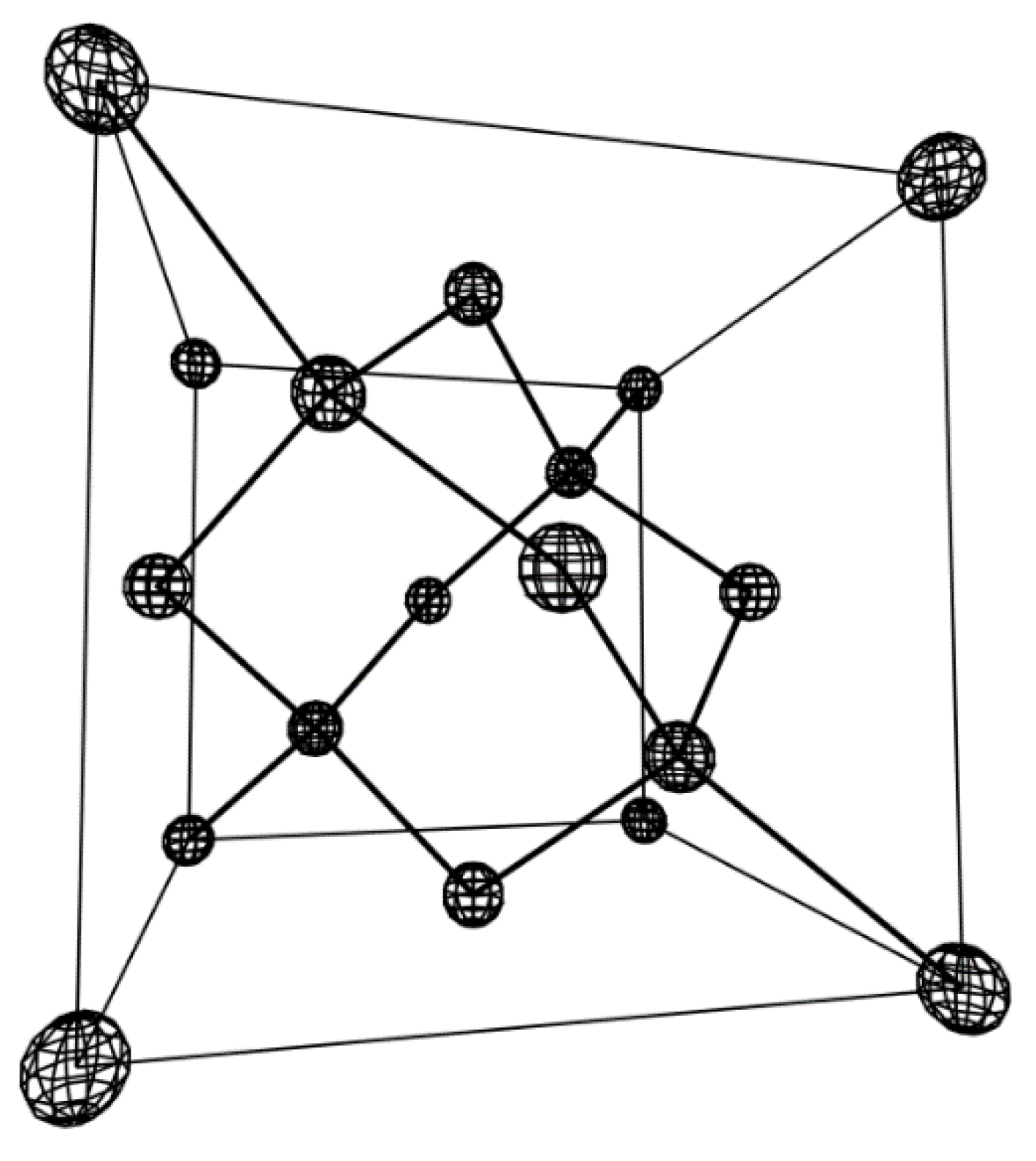
Consider crystalline silicon as a typical material. The simulated sample is represented by eight unit cells of a diamond crystal lattice making up a cube of $2\times 2\times 2$ in size, with periodic boundary conditions; each unit cell contains eight unique atoms (Figure 14), so a total of 64 atoms are involved in the simulation. Initial speeds are considered to be zero. The initial conditions for a dynamical system can be represented as follows:

$$\{\begin{array}{l}{r}_i(0)=\left({\left(x,y,z\right)}^T+{\left(dx,dy,dz\right)}^T\right)a,\hspace{0.17em}\left(x,y,z\right)\in \mathrm{Base},\hspace{0.17em}dx,dy,dz\in \left\{0,1\right\},\hspace{0.17em}{v}_i(0)={\left(0,0,0\right)}^T,\\ Base=\left\{\begin{array}{l}\left(0,0,0\right),\hspace{0.17em}\left(0,0.5,0.5\right),\hspace{0.17em}\left(0.5,0,0.5\right),\hspace{0.17em}\left(0.5,0.5,0\right),\left(0.75,0.75,0.75\right),\hspace{0.17em}\\ \left(0.75,0.25,0.25\right),\hspace{0.17em}\left(0.25,0.75,0.25\right),\left(0.25,0.25,0.75\right)\hspace{0.17em}\hspace{0.17em}\end{array}\right\},\end{array}$$

where $a=5.429\times {10}^{-10}\hspace{0.17em}\mathrm{m}$ is the linear size of a unit cell of a silicon crystal.

To take into account deformation, 4 additional variables are introduced: one of them reflects the elongation value, and three more are responsible for the angle between the orientation of the lattice and the direction of stretching. In this case, the elongation is set to be fixed, and the variables responsible for the rotation are taken as interval. Rotation is generated evenly using quaternions [28].

The final system looks like this:

$$\{\begin{array}{l}{r}_i{}^{\prime }=v_i,\hspace{0.17em}{v}_i{}^{\prime }=-\frac{1}{2m_i}{\displaystyle \sum _i{\displaystyle \sum _{j\ne i}{\nabla }_i\left(f_C\left(r_{ij}\right)\left(f_R\left(r_{ij}\right)+b_{ij}{f}_A\left(r_{ij}\right)\right)\right)}},\\ r_{ij}\left(s,{\mu }_1,{\mu }_2,{\mu }_3\right)=\Vert S\left(s\right)R\left({\mu }_1,{\mu }_2,{\mu }_3\right)r_{ij}\Vert ,\\ S(s)=\mathrm{diag}(1+s,1,1),\\ R\left({\mu }_1,{\mu }_2,{\mu }_3\right)=\left(\begin{array}{ccc}1-2\left(q_2^2+q_3^2\right)& 2\left(q_1{q}_2-q_3{q}_0\right)& 2\left(q_1{q}_3+q_2{q}_0\right)\\ 2\left(q_1{q}_2+q_3{q}_0\right)& 1-2\left(q_1^2+q_3^2\right)& 2\left(q_2{q}_3-q_1{q}_0\right)\\ 2\left(q_1{q}_3-q_2{q}_0\right)& 2\left(q_2{q}_3+q_1{q}_0\right)& 1-2\left(q_1^2+q_2^2\right)\end{array}\right),\\ \left(q_0,q_1,q_2,q_3\right)=\left(\sqrt{1-{\mu }_1}\sin \left(2\pi {\mu }_2\right),\sqrt{1-{\mu }_1}\cos \left(2\pi {\mu }_2\right),\sqrt{{\mu }_1}\sin \left(2\pi {\mu }_3\right),\sqrt{{\mu }_1}\sin \left(2\pi {\mu }_3\right)\right),\\ t\in \left[0,{10}^{-12}\right],\end{array}$$

(13)

where $m=4.65\times {10}^{-26}\hspace{0.17em}\mathrm{kg}$ is the mass of atoms, $s=0.1$ is the relative elongation of the sample, ${\mu }_1\in [0.1,0.9]$, ${\mu }_2\in [0.1,0.9]$, and ${\mu }_3\in [0.1,0.9]$ are stretching direction parameters, $R=2.85\times {10}^{-10}\hspace{0.17em}\mathrm{m}$, $D=0.15\times {10}^{-10}\hspace{0.17em}\mathrm{m}$, $A=6.12\times {10}^{-16}\hspace{0.17em}\mathrm{J}$, $B=1.81\times {10}^{-17}\hspace{0.17em}\mathrm{J}$, $c=9.69$, $d=2.35$, $n=4.16$, $\beta =0.132$, ${\lambda }_1=3.36\times {10}^{10}\hspace{0.17em}{\mathrm{m}}^{-1}$, ${\lambda }_2=1.27\times {10}^{10}\hspace{0.17em}{\mathrm{m}}^{-1}$, ${\lambda }_3=1.19\times {10}^{10}\hspace{0.17em}{\mathrm{m}}^{-1}$, $\gamma =5.71$, and $\cos ({\theta }_0)=-0.408$ are the parameters of the potential.

Integration of the resulting ordinary differential system (13) was carried out using the Verlet velocity method with a constant integration step of ${10}^{-15}\hspace{0.17em}\mathrm{s}$. As a result, the interval stress tensor was obtained (values are given in Pascals):

$$\left(\begin{array}{ccc}[-1.58\times {10}^{10},-1.43\times {10}^{10}]& [-1.35\times {10}^9,1.35\times {10}^9]& [-1.35\times {10}^9,1.35\times {10}^9]\\ [-1.35\times {10}^9,1.35\times {10}^9]& [-4.79\times {10}^9,-1.46\times {10}^9]& [-1.42\times {10}^9,1.42\times {10}^9]\\ [-1.35\times {10}^9,1.35\times {10}^9]& [-1.42\times {10}^9,1.42\times {10}^9]& [-4.79\times {10}^9,-1.46\times {10}^9]\end{array}\right)$$

For $\epsilon ={10}^{-2}$, the obtained result was $I=1079132.3$ and $error=2\times {10}^{-1}$.

Note that the possibilities of the proposed approach are not limited to a specific type of interatomic interaction potential in a material. The method can be applied to the simulation of the stress–strain state of materials with various types of chemical bonds, including the modeling of composite materials.

5. Discussion

In the previous sections, the proposed approach was tested on representative interval problems of nonlinear dynamics and computational materials science. It is found that, thanks to sparse grids, it is possible to integrate ODE systems with a large number of interval uncertainties in a reasonable time. To estimate the computational costs, a criterion was used that is equal to the equivalent number of sampling points from the original uncertainty region.

Table 1 shows estimates of the computational costs for the ODE system given by Equation (9) describing a conservative oscillator with two interval initial conditions for two values $\epsilon$. For $\epsilon ={10}^{-3}$, the approach proposed in the paper works $1.5$ to $5$ times faster than the classical adaptive interpolation algorithm.

Table 2 shows the computational costs when integrating the ODE system given by Equation (10), describing the Lotka-Volterra model with two interval initial conditions and one interval parameter. Here, for $\epsilon ={10}^{-3}$, the use of adaptive sparse grids gives an acceleration of $1.9-2.8$ times compared to the classical algorithm, and for $\epsilon ={10}^{-5}$, the acceleration is from $1.25$ time to $15$ time.

For ODE systems given by Equations (11) and (12), it was possible to obtain a solution in a reasonable time only using the approach proposed in the paper since the number of interval uncertainties is quite large. To solve system given by Equation (11), the equivalent number of sampling points was about $80$ thousand, and in the case of using the classical algorithm with a degree of polynomial $4$, the value would be about $10$ million. Thus, using sparse grids in this problem gives an acceleration of at least $125$ times.

The tables show that adaptive sparse grids work faster than regular sparse grids, and even faster than full grids. This fact is in line with the theoretical foundations. The classical adaptive interpolation algorithm in example (9) with two interval uncertainties showed itself slightly better only when $\epsilon ={10}^{-5}$ and $p=4$. This is primarily due to the chosen value of p. It is known that the greater the degree of the interpolation polynomial, the faster the error decreases with increasing mesh density. Therefore, it seems promising to use sparse grids on a nonlinear basis. We should also note the possibilities of applying adaptive grids to ODE systems not only with interval uncertainties but also with stochastic uncertainties, including applied nonlinear systems.

6. Conclusions

The adaptive interpolation algorithm allows simulating dynamic systems with interval parameters. In the course of the algorithm operation, a regular grid is constructed in the parameter space. The number of grid nodes depends exponentially on the number of interval parameters, which limits the scope of the algorithm. A typical situation is when the degree of influence of different parameters and their combinations on the solution can differ significantly. This can be used in adaptive interpolation. The paper presents an adaptive interpolation algorithm on sparse grids, which allows for reducing the exponential complexity when solving multidimensional problems in parameter space. The efficiency of the proposed approach has been demonstrated on representative interval problems of nonlinear dynamics and computational materials science. It is shown that, for most variants, adaptive sparse grids are more efficient than the classical adaptive interpolation algorithm in terms of computational costs. With the suggested method, it was possible to solve problems with up to 10 interval parameters in a reasonable amount of time. At the same time, the classical algorithm of adaptive interpolation failed to do so. Taking into account that an increase in the degree of the interpolation polynomial in the classical adaptive interpolation algorithm leads to higher accuracy and lower computational costs, we can outline the use of sparse grids with a nonlinear basis as a direction for further research.