Fluid-Flow Approximation in the Analysis of Vast Energy-Aware Networks

Abstract

The paper addresses two issues: (i) modeling dynamic flows transmitted in vast TCP/IP networks and (ii) modeling the impact of energy-saving algorithms. The approach is based on the fluid-flow approximation, which applies first-order differential equations to analyze the evolution of queues and flows. We demonstrate that the effective implementation of this method overcomes the constraints of storing large data in numerical solutions of transient problems in vast network topologies. The model is implemented and executed directly in a database system. It can analyze transient states in topologies of more than 100,000 nodes, i.e., the size which was not considered until now. We use it to investigate the impact of an energy-saving algorithm on the performance of a vast network. We find that it reduces network congestion and save energy costs but significantly lower network throughput.

1. Introduction

The size of the Internet is exponentially increasing, reaching 5168 million users in March 2021 [1]. Since 2010, global Internet traffic has increased 15-fold, or  30% per year (40% in 2020) [2]. Understanding the behavior of this complex system is of critical importance; yet, modeling it is a challenge. We need tools to help us better understand and predict the effects of changes concerning the Internet’s configuration, load, and traffic control algorithms. We should model the impact of network parameters on the quality of transmissions and energy consumption. The latter is an important problem; globally, data transmission networks consumed 260–340 TWh in 2020, or 1.1–1.4% of global electricity use [2,3]. There is a constant effort to improve the energy efficiency of these networks; fixed-line network energy intensity measured in kWh/GB has halved every two years since 2000 in developed countries, and mobile-access network energy efficiency has improved 10–30% annually in recent years [2].

Performance evaluation techniques for communication networks are based on discrete-event simulation, experiments, or mathematical analysis [4].

There are well-tested tools such as ns-2, in [5], ns-3, in [6], or OMNet++, in [7], for discrete-event simulations. They may model many specific protocols and network types on packet-level, i.e., simulator mimics the behavior of every packet in a network, but their capabilities fall behind the Internet size. Moreover, if we want to see the effects of traffic control decisions, transient analysis is needed. It means repeating the simulation many times to obtain statistics for specific moments in time and is highly time-consuming.

In experiments, the network under study is constructed using real devices and computers. It enables a detailed performance evaluation, but it generally lacks flexibility and requires significant effort and cost to build the actual system; it is unrealistic in the case of the Internet.

Therefore, the approach based on the mathematical description, even if it is simplified, is adopted by many authors, e.g., [8,9,10]. It was used mainly to study the quality and stability of traffic control algorithms, e.g., TCP/IP congestion window mechanism. We apply it to investigate energy consumption issues.

In practice, three analytical approaches may analyze transient states: numerically solved Markov models, diffusion approximation, and fluid-flow approximation, see [11]. Below we discuss their choice.

The Markov chains were used by Erlang [12] and Engset [13] for the analysis of early telecommunication systems, and remain a standard tool of queuing theory and performance evaluation. They may model complex features of Internet traffic, such as self-similarity and long-range dependence, e.g., [14], and serve well in the evaluation of single IP routers [15]. However, similarly to discrete-event simulation models, they describe a network on the packet level; therefore their possibilities are limited by the explosion of states. Each state of a Markov chain corresponds to the state of an investigated system. State probabilities are obtained by solving the Chapman–Kolmogorov equations, which are algebraic in the case of steady-state analysis and differential in the case of the transient one. The appropriate numerical methods [16] and specialized software [17,18] are continuously being developed and allow us to solve systems of the size of hundreds of millions of equations. However, it is still insufficient to model Internet configurations.

Therefore, we need to apply methods such as diffusion approximation or fluid-flow approximation, which refer to changes in flow intensity and may be used to investigate much larger topologies.

The method of diffusion approximation was introduced by Gelenbe [19] and Kobayashi [20]; then the authors of [21] studied its numerical side. In this method, the number of customers in a queuing system is approximated by the value of the diffusion process. The density function of the process is obtained by solving a second-order partial differential equation with parameters depending on the mean and variance of the interarrival and service time distributions in the considered queuing system. This density corresponds to the time-dependent queue distribution [11,21]. The size of the considered networks may be much larger than in Markov models; in [22] we analyzed with the diffusion approximation a network having 1000 nodes. However, due to complex computations, the method cannot be applied to Internet topology.

Because of the above constraints, we decided to implement models based on the fluid-flow approximation. This simplified approach was introduced by Moran [23] to study water reservoirs and storage systems and then adopted by computer science. It was used for the analysis of computer networks in a series of articles by Towsley and his group, e.g., [8,9] and then e.g., by Sakumoto et al. [10]. It is a first-order approximation; the time-dependent flows and queues are represented only by their mean values and linked by first-order differential equations. Therefore, it is less accurate than the diffusion approximation; a numerical comparison of diffusion and fluid-flow methods modeling transient states was presented in [24].

The simplicity of fluid-flow approximation allows us to build models of much larger networks and makes it possible to implement the basic principles of traffic control applied in TCP/IP stack. Implementing such models, we discovered that their computational bottleneck is not in the numerical solution of a massive system of equations but in storing and retrieving intermediate results needed in the transient analysis where the current state of the network depends on the network’s history. Therefore, we built a practical implementation of the fluid-flow model inside a professional database system. A few issues of this approach and its usage were previously discussed in [25,26,27,28]. Here, we concentrate on modeling energy-aware nodes that fall asleep when their queues are small. The model gives us information on the effects of this policy on the performance of a large-scale network.

The contributions of the article are as follows.

(i)

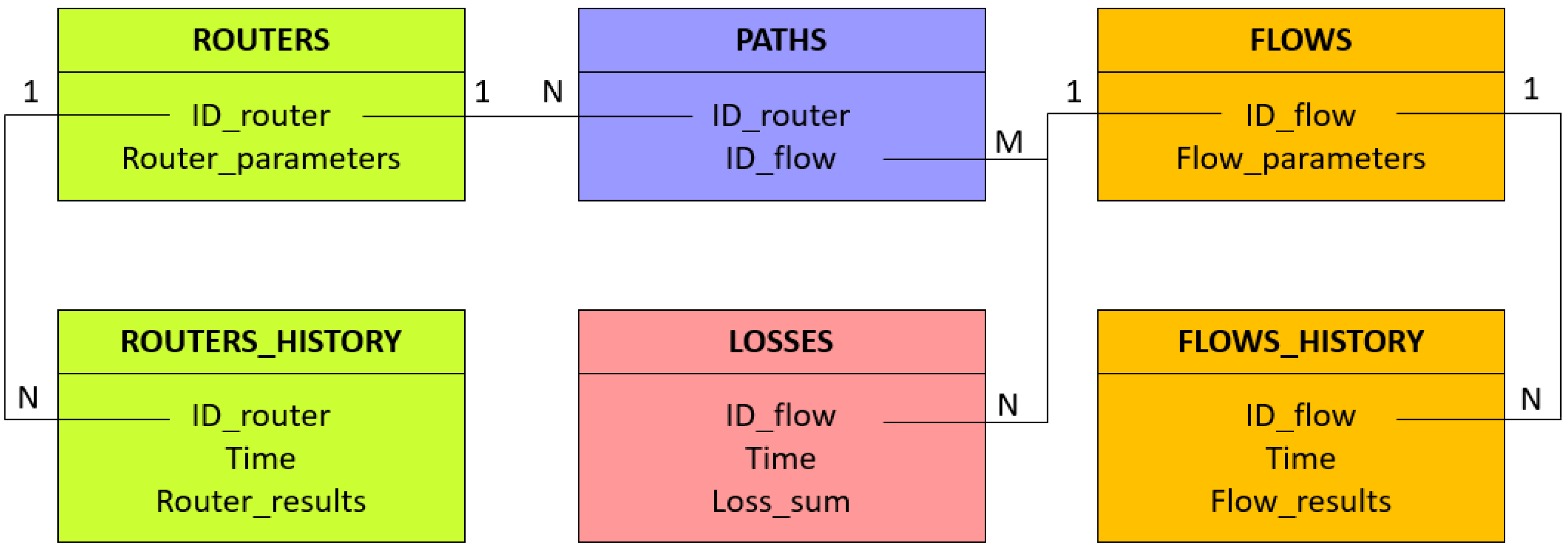
we develop a queuing model of an extensive computer network. The model captures the dynamics of flows changing due to the nature of transmitted traffic and the network’s control algorithms. We consider the TCP Reno algorithm cooperating with the RED algorithm on IP level, but they may be easily replaced by other algorithms. The model is based on the well-known fluid-flow approximation. Its original part is the implementation of the whole structure inside the database system. This is the way to overcome the limitations of storing and using large amounts of data resulting from the size of the model and the analysis of transients. This unconventional solution allows us to model previously inaccessible topologies related to the Internet.

(ii)

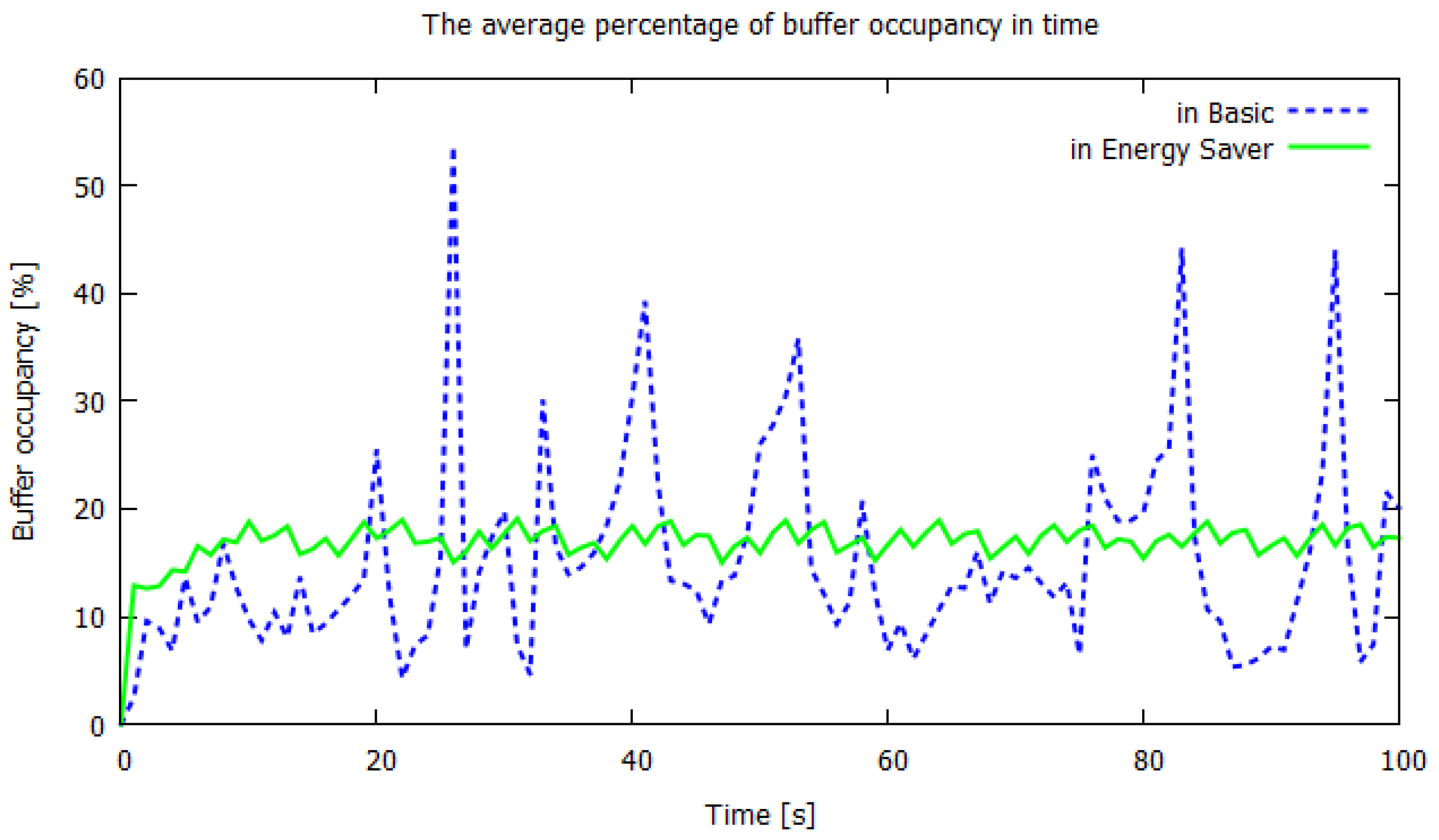
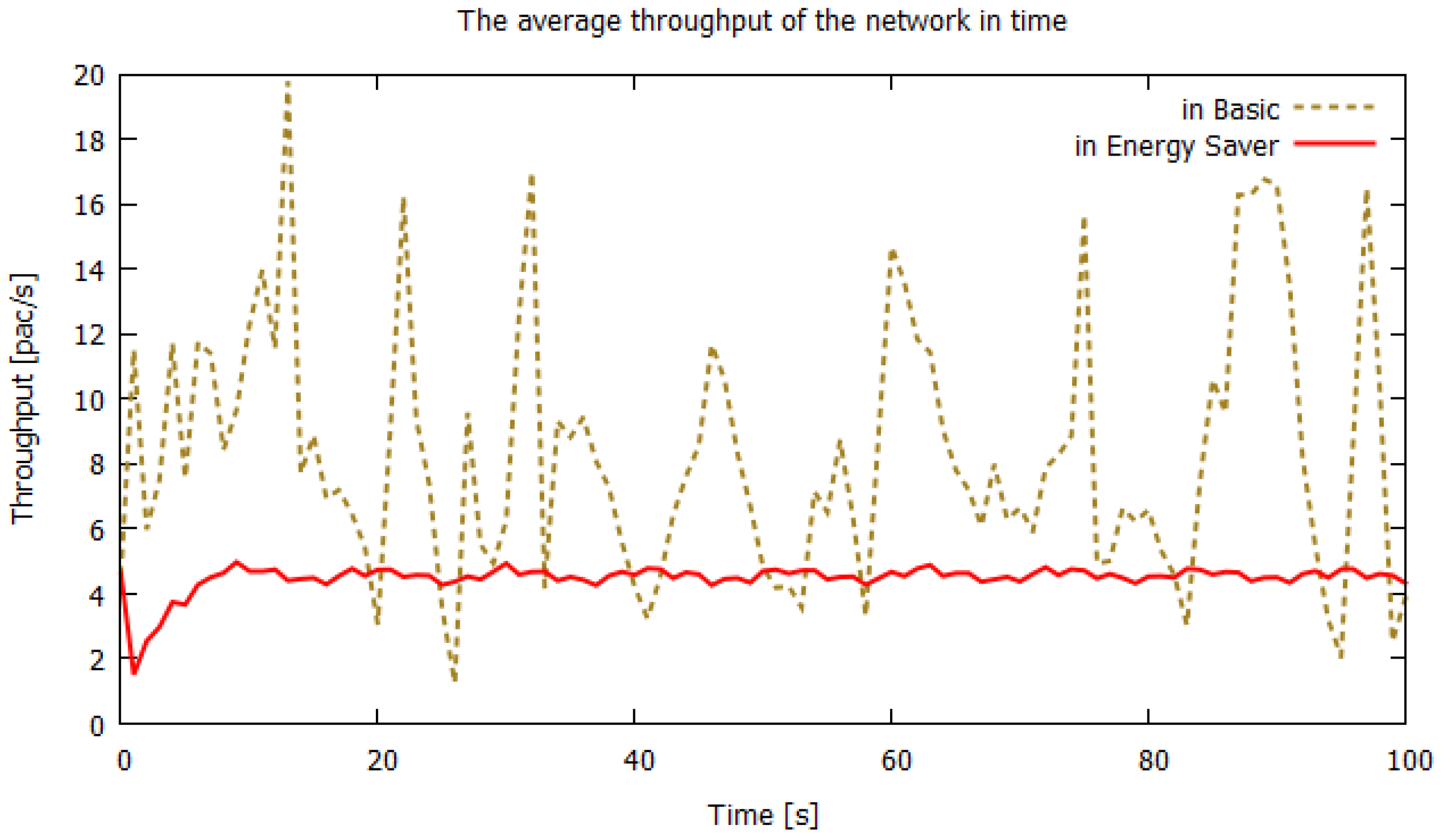
we apply this model in the quantitative analysis of the impact of an energy-saving algorithm used in routers on the network’s performance. We discover that it reduces network congestion and save energy but significantly lowers network throughput. The studied network has a realistic hierarchical, nonhomogenous structure with routers and links of various throughputs and buffer sizes and is a copy of an existing part of the Internet; it was taken from a map developed in the Opte project in [29].

The rest of the article is organized in the following way. Section 2 gives a brief review of recent works on green networks solutions and fluid-flow applications. Section 3 provides the basic model of the fluid-flow approximation in the case of an arbitrary topology network and introduces our energy-saving node model. Section 4 presents the model’s implementation details and obtained results illustrating the impact of the energy-saving policy on the performance of a vast network. We also give the model execution times and memory consumption. Conclusions are in Section 5.

2. Related Works

A continuous increase in the number of clients or end-user devices connected to a network [30] makes it necessary to concentrate on the topic of energy consumption and its impact on the quality of the provided services. Energy consumption is important both for individual devices and for the entire system. The literature describes energy-aware sensors (e.g., [31]), mobile networks (e.g., [32]), and wireless networks (e.g., [33]). For data centers and cloud computing, energy saving is also a significant issue in terms of economic and environmental reasons: the lack of energy efficiency results in a loss of profitability [34] and waste of energy. Attention also goes to software energy consumption, [35]. The common assumption that it is enough to limit CPU consumption to save energy turned out to be inadequate; see the results of [36] where a software tool allows monitoring the energy consumption provided by Intel’s CPUs for verification algorithms. The biggest concerns, however, are raised by cryptocurrencies. Reference [37] illustrates the steady increase in energy consumption during cryptocurrency mining and points out the environmental hazards in this area. Therefore, many energy-saving areas are being explored. Following the development of edge computing, cloud computing, and 5G networks, the most recent focus includes migration methods and scheduling certain tasks from local devices to remote cloud processing [38,39], energy management systems focused on security [40], task allocation algorithms in multi-cloud networks [41], and energy-aware video streaming for mobile devices [42,43]. Increasingly more works are also related to energy saving in the context of Internet of Things networks, e.g., [44,45,46].

To the best of our knowledge, one of the first attempts to build a unit of a green primary network was [47]. The authors identified the need to redesign the wired network hardware to make the router more energy efficient. The work was part of the ECONET project, where 13 prototypes of network devices were developed that enable energy savings. The paper focuses on one of the prototypes that can aggregate multiple data planes of software routers. The implementation reduced energy consumption while maintaining satisfactory performance. In the same project, the paper [48] studies the impact of TCP transmission on the energy efficiency of network devices. On the basis of the analysis of real measurements over multiple TCP connections and variants, the work defines key indicators in terms of energy and performance. It shows the impact of network scenarios and TCP variants on the total energy consumed by network devices. Similarly, [49] analyzes the impact of TCP network congestion traffic on the energy efficiency of end hosts. The paper describes the significant energy gains from reducing the number of losses and retransmissions of the TCP protocol. Several articles also introduce and investigate modifications to transmission mechanisms or variants of TCP protocols, making them energy-saving while preserving or increasing their performance, e.g., [50,51,52,53,54,55]. Reference [56], in turn, focuses on energy consumption during the idle state. It proposes an algorithm to reduce power consumption by bringing a router without associated clients into a sleep state instead of an idle mode. The simulation results confirmed the assumed improvement in energy consumption.

In addition, queuing models can be applied to evaluate the impact of an energy-saving configuration on the overall energy consumption in data centers. In [57,58], a data center is represented as a queuing system with homogeneous servers and a central queue. The servers work according to the specific policy; they switch on or off depending on the number of jobs in the system to ensure the expected energy cost. The topic is continued in [59], where a data center is represented as a fluid-flow system. Energy consumption depends on the achievement of the defined thresholds of the buffer capacity. A review of existing data centers modeled as queuing systems, including classical and energy-aware performance, can be found in [60]. A general model of energy-aware server based on M/G/1 queue is shown in [61]. In the case of network nodes, the authors of [62] study the use of queuing theory to identify the number of bands needed to service the incoming traffic in multi-band WiFi routers; unused bands are put into a sleep mode to save energy.

A single node model using the fluid-flow approximation of the TCP connection was shown in [9]. In addition to a differential equation representing changes in the router queue length, another was specified that describes the window size. The model is also enriched with equations defining round trip time, the Active Queue Management (AQM) policy, and a proposal for aggregating identical flows and timeout losses. A method to extend the model to a network case was also indicated. Finally, the modeling results are compared with the simulation. The article [8] introduces to the above model the order of stations making a specified connection. It considers various AQM schemes and TCP variants such as Reno, New Reno, and SACK. It also reduces the computational complexity of the model by eliminating nodes that are not overloaded in the topology, ensuring this way the scalability of the model. Another model following this approach incorporates short- and long-term transient TCP flows [63]. The work considers the size of the congestion window in both the slow start and congestion avoidance phases. It provides differential equations that regulate the behavior of the threshold parameter and the average amount of data sent by the source. All these works refer either to a single node or to a small network of several nodes.

3. Fluid-Flow Approximation

3.1. Basic Model

The fluid approximation [8,9] uses first-order ordinary linear differential equations to determine the average values of the node queues and the dynamics of TCP congestion windows in a modeled network.

Consider a network of N nodes and K flows. Changes in the mean queue size $q_j$ at a node j are defined in Equation (1) by the balance of the intensities of the input stream, i.e., the sum of all flows $l_i\left(t\right)$ entering the node, and the output flow, i.e., the constant number $C_j$ of packets forwarded in a time unit, provided that the queue is not empty,

$$\frac{{\mathit{dq}}_j\left(t\right)}{\mathit{dt}}=\sum _{i\in K_j}{l}_i\left(t\right)-\mathcal{H}(q_j\left(t\right)>0)C_j,$$

(1)

where $\mathcal{H}\left(x\right)$ is Heavyside peacewise function, $\mathcal{H}\left(x\right)=1$ for $x>0$ and $\mathcal{H}\left(x\right)=0$ for $x\le 0$.

The intensity of flows is controlled by the size of TCP congestion window

$$l_i\left(t\right)=\frac{W_i\left(t\right)}{R_i\left(q_i\left(t\right)\right)}$$

(2)

where

-

$W_i\left(t\right)$ is the size of congestion window for connection i, i.e., the number of packets (or more precisely blocks) the sender is allowed to dispatch without waiting for acknowledgment of reception from the receiver;

-

$R_i\left(q_i\left(t\right)\right)$ is the round trip time for a flow i, i.e, the mean time after which such acknowledgment is received.

All model parameters are shown in

Table 1. Notations used in the paper.

Element	Parameter	Meaning
Node	N	Total number of nodes
	$q_j$	Current queue size at j-th node
	$C_j$	Output flow of j-th node
	$p_{ij}$	Loss probability at j-th node for i-th flow
	$x_j$	Weighted average queue length at j-th node
	$t_{mi{n}_j}$	Lower threshold for $x_j$ queue
	$t_{ma{x}_j}$	Upper threshold for $x_j$ queue
	$p_{ma{x}_j}$	Maximum loss probability at upper threshold for $x_j$ queue
	$w_j$	Weight for $x_j$ queue
	$T_A$	Lower threshold that switch off router’s service
	$T_B$	Upper threshold that switch on router’s service
Flow	K	Total number of flows
	$K_j$	Set of flows crossing node j
	$l_j$	Throughput of input stream of j-th node
	$W_i$	Congestion window size of i-th flow
	$R_i$	Round trip time of i-th flow
	$q_i$	Set of current queues at i-th connection
	$V_i$	Set of nodes for i-th connection
	$T_i$	Propagation time between i-th and $(i+1)$-th nodes
	$L_i$	Set of links for i-th connection
	$N_i$	Number of identical flows at j-th node
Time	t	t-th time step
	$\Delta t$	Time length of a time step
	$\tau$	Time when the loss occurred
Mode	$N-mode$	Normal mode
	$ES-mode$	Energy-saving mode

. In the following paragraph, all parameters presented in Table 1 are described in detail.

The round trip time is computed as

$$R_i\left(q_i\left(t\right)\right)=\sum _{j\in V_i}\frac{q_j\left(t\right)}{C_j}+\sum _{j\in L_i}{T}_j.$$

(3)

where

-

$q_i$ is the set of mean queues in connection i,

-

$V_i$ is the set of nodes belonging to the connection i,

-

$T_j$ is the propagation time between two nodes j, $j+1$,

-

$L_i$ is the set of links between the nodes belonging to connection i.

Following TCP principles, the intensity of each flow i is determined by a time-varying congestion window size $W_i$ kept by the sender of this flow. Equation (4) presents the changes of the congestion window due to the basic Reno algorithm. It is no longer widely used but serves as a reference in the performance evaluation of various newer variants of TCP [64,65,66,67,68]. Following the original papers on fluid-flow approximation, we concentrate here on the performance of Reno during the congestion avoidance phase. At the same time, we prepare model extensions, including slow start and fast retransmit/fast recovery phases, and another protocol may replace Reno itself.

The window size increases by one each round trip time in the absence of packet losses (first term on the right side of Equation (4)) and decreases by half its current value, with a delay $\tau$ (the sender is not immediately aware of the loss), after each packet loss occurs in nodes on the flow path (the next term in Equation (4)). The intensity of losses for each TCP connection is computed as the flow of packets,

$$\frac{W_i(t-\tau )}{R_i\left(q_i(t-\tau )\right)}$$

multiplied by the probability that a packet is lost at any node on its way. Therefore, the changes in congestion window size are defined as follows:

$$\frac{{\mathit{dW}}_i\left(t\right)}{\mathit{dt}}=\frac{1}{R_i\left(q\left(t\right)\right)}-\frac{W_i\left(t\right)}{2}·\frac{W_i(t-\tau )}{R_i\left(q_i(t-\tau )\right)}·\left(1-\prod _{j\in V_i}(1-p_{ij})\right),$$

(4)

where $p_{ij}$ is the loss probability for packets of flow i at node j.

In AQM mechanisms used to control TCP/IP connections, a packet may be dropped even if there is still a place to store it at a node. The drop probability $p\left(x_k\right)$ of a k-th packet at any node is given by Equation (6). It is determined according to the well-known Random Early Detection (RED) mechanism [69,70] as a function of the weighted moving average of the queue length, Equation (5), where $x_k$ is the weighted average queue determined at the arrival of the k-th packet, $x_{k-1}$ is the average calculated at the arrival of the previous packet, $q_k$ is the queue length at the arrival of packet k, and $0<w<1$ is a parameter that determines the balance between the history and the current state of the queue taken into account in the control mechanism. We may see this average as a low-pass filter, eliminating short-time changes of the queue and enhancing the long-time trends.

$$x_k=w{x}_{k-1}+(1-w)q_k.$$

(5)

There is no simple recipe for choosing the weight w (neither for thresholds $t_{\mathit{min}}$ and $t_{\mathit{max}}$ in Equation (6)), it depends on the type of traffic and its dynamics, see remarks in [71,72]. In our model, we take a typical value $w=0.95$. In a real network, the moving average is determined by the arrivals of packets; here in the model, it is updated in fixed intervals of $\Delta =0.1$ s, when all model parameters are refreshed.

Changes in $p\left(x_k\right)$ are linear between thresholds $t_{\mathit{min}}$, $t_{\mathit{max}}$. Below the lower threshold, there is no loss, and above the upper one, all packets are deleted.

$$p\left(x_k\right)=\left\{\begin{array}{cc}0,& 0⩽x_k<t_{\mathit{min}}\\ {\displaystyle \frac{x_k-t_{\mathit{min}}}{t_{\mathit{max}}-t_{\mathit{min}}}{p}_{\mathit{max}},}& t_{\mathit{min}}⩽x_k⩽t_{\mathit{max}}\\ 1,& t_{\mathit{max}}<x_k.\end{array}\right.$$

(6)

3.2. Fluid-Flow Approximation of an Energy-Efficient Node

We assume here that the router is either in a normal operating mode or in an energy-saving one. It could be possible, e.g., in the SDN environment, by defining rules for switching between the modes in individual nodes. The data on the current load are sent through the SDN control–data-plane interface to the SDN controller, which decides on the working mode. Here, when the router is in energy-saving mode, it is not servicing packets, but it collects them in the buffer. We introduce two independent thresholds for queue length. They define the operating mode of the router in the following way:

• When the actual queue length q decreases and reaches the lower threshold of $T_A$, the router service is switched off. This results in the growth of the router queue.
• When the actual queue q increases and reaches the upper threshold of $T_B>T_A$, the router service is switched on. It is the moment when we assume that the router has a long enough queue to start transmitting.
• In other cases, the state of the router does not change.

The introduction of hysteresis $T_B-T_A$ prevents the router from constantly switching between the two modes of operation. Equation (1) becomes

$$\frac{{\mathit{dq}}_j\left(t\right)}{\mathit{dt}}=\left\{\begin{array}{cc}{\displaystyle \sum _{i=1}^K\frac{W_i\left(t\right)}{R_i\left(q\left(t\right)\right)}·N_i-\mathcal{H}(q_j\left(t\right)>0)·C_j,}& q⩾T_B\\ {\displaystyle \sum _{i=1}^K\frac{W_i\left(t\right)}{R_i\left(q\left(t\right)\right)}·N_i}& q⩽T_A\\ {\displaystyle \sum _{i=1}^K\frac{W_i\left(t\right)}{R_i\left(q\left(t\right)\right)}·N_i-\mathcal{H}(q_j\left(t\right)>0)·C_j,}& q>T_A,N-mode\\ {\displaystyle \sum _{i=1}^K\frac{W_i\left(t\right)}{R_i\left(q\left(t\right)\right)}·N_i}& q<T_B,ES-mode\end{array}\right.$$

(7)

where N-mode is the normal mode and ES-mode is energy-saving mode.

4. Implementation and Numerical Results

We compare two networks of the same topology, transmitting the same flows: one is composed of standard routers (a basic model) and the other of energy-aware routers (energy-saving model). To implement and compare both network models, we used the in-memory database SAP HANA [73]. The calculations were performed on 1 TB SAP HANA Appliance. The models were implemented in the Structured Query Language (SQL) as a database procedure consisting of an initial step and a stepwise loop over predefined time. The network parameters (topology structure, RED parameters, initial queues, nodes capacities, initial TCP windows sizes) were loaded from CSV files into dedicated database tables, Figure 1, in the initial phase.

For router and flow parameters, we defined the ROUTERS and FLOWS table. They stored the values of the current step (q, x, p, W, R, l, N) and fixed parameters (C, $t_{min}$, $t_{max}$, $p_{max}$, w, T). The previous steps were collected in the ROUTERS_HISTORY and FLOWS_HISTORY tables. For each flow, the loss values were saved into the LOSSES table. This table acted as a table with current and historical data. The structures of the network were preserved in the PATHS table.

With each modeling step, the nodes and flows parameters were updated. Algorithm 1 consists of two types of blocks: calculations and saves. Within the calculation block, we used the UPDATE FROM SELECT statement, which first calculated all parameters for each router/flow using the ROUTERS/FLOWS table using nested SELECTs and then UPDATE the corresponding rows with those values. The save block was made using the INSERT FROM SELECT statement, which writes the result rows into the ROUTERS_HISTORY/FLOWS_ HISTORY table. Similarly, we calculated and saved losses, however, using the UPSERT FROM SELECT statement, which updated the value in LOSSES table when it has previously been present or inserted a new value otherwise. The energy-saving modifications of the basic model, see Algorithm 2, were made within $CalculateAllParametersForAllRotuers$.

Algorithm 1: Fluid-flow approximation written as a database procedure

Algorithm 2: Energy-saving modification of fluid-flow approximation

As the modeling results, we obtained two groups of data, which were then queried to extract the specific values of interest. The data were then plotted using the Gnuplot [74] or Gephi [75] tools to visualize the characteristics.

We remark that the Structured Query Language, which is a domain-specific language designed for managing data held in a relational database management system, may be used not only for data manipulation but also—with much success—for numerical calculations. The use of a database is essential for this implementation because it facilitates the processing of large amounts of data necessary for the analysis of transient states. All results are stored in the database, and SQL queries may highlight any desired aspect of the network performance.

To compare the performance of both networks, we used an exemplary topology, [29], with 134 thousand nodes and 50 thousand flows that traverse the network. The method of topology extraction is described in [76].

Considering a topology of this size, we have nearly 9.5 GB and 10 GB of data to compare. Individual sizes are listed in

Table 2. Comparison of the number of rows, memory, and disk size for the basic (B) and energy-saving (E) models.

Table	No of Entries	Memory Size (KB)	Disk Size (KB)
FLOWS_B	50,000	4201	4460
FLOWS_E	50,000	4217	4468
FLOWS_HISTORY_B	50,050,000	3,939,782	3,863,984
FLOWS_HISTORY_E	50,050,000	3,997,634	3,832,560
ROUTERS_B	134,023	4706	4800
ROUTERS_E	134,023	4806	4944
ROUTERS_HISTORY_B	134,157,023	3,698,226	3,567,340
ROUTERS_HISTORY_E	134,157,023	3,967,444	3,788,272
LOSSES_B	44,559,219	1,905,595	1900 128
LOSSES_E	45,721,414	2,020,755	1,936,288

.

The initial values of queue lengths were set to zero, and the initial sizes of the congestion windows were set to one. The nodes were not homogeneous; their parameters were chosen based on the volume of traffic they transmitted. The buffer volume (maximum queue) B was in the range $B\in [15;\mathrm{469,785}]$ packets, and the speed of node $C\in [1125;\mathrm{99,933}]$ packets/s. In energy-saving mode, we set the C-disabling thresholds $T_A$ to 20% of B and $T_B$ to 25% of B. The rest of the parameters remained the same as in normal mode. All presented results are based on the samples collected for each second of modeling time.

The first set of results presents the percent of the idle time of the routers when they are not transmitting ($C=0$ or $q=0$) in normal mode, Figure 2, and in energy-saving mode, Figure 3. Here we do not preserve the network topology. The meaning of colors is as follows:

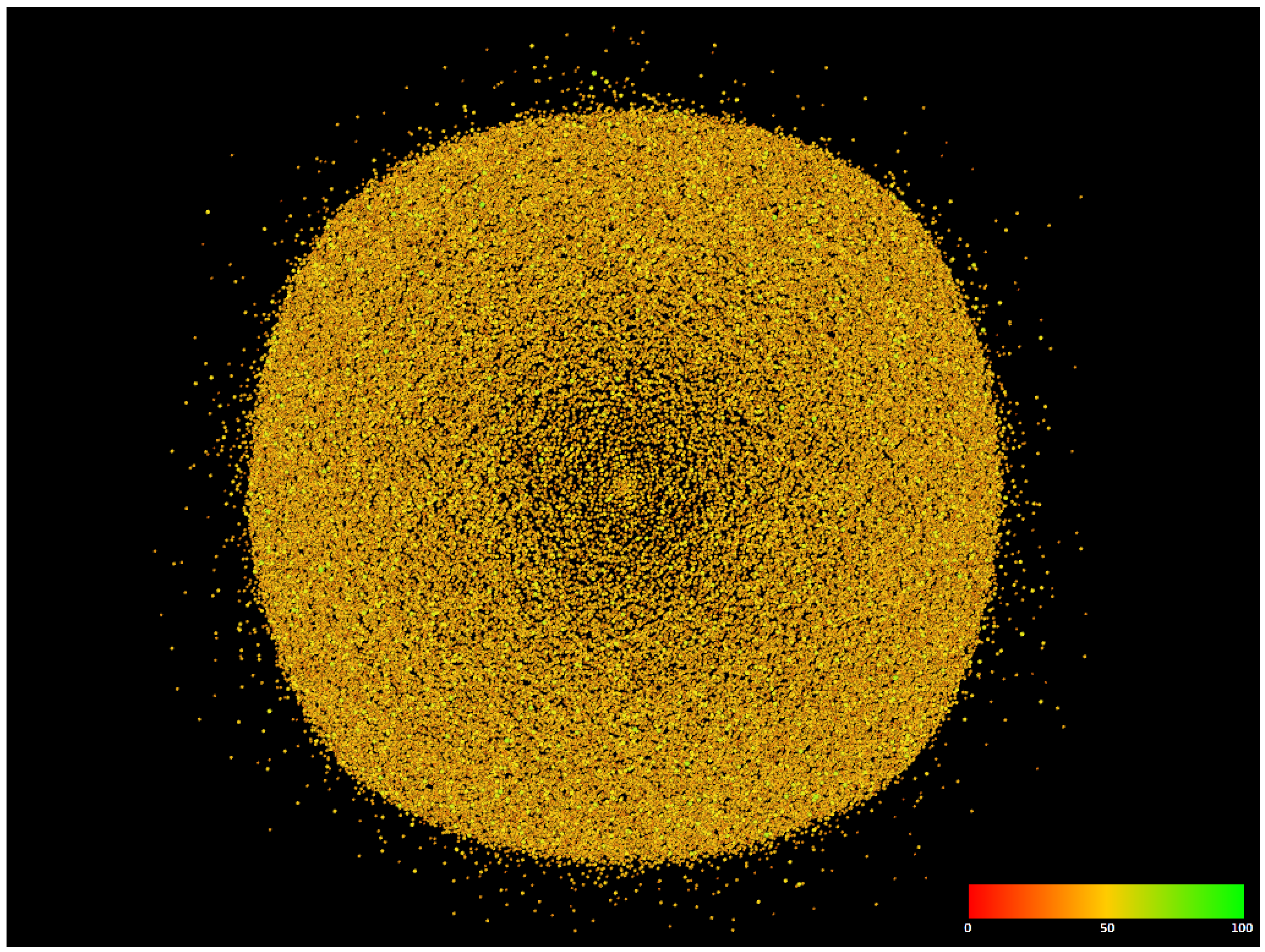
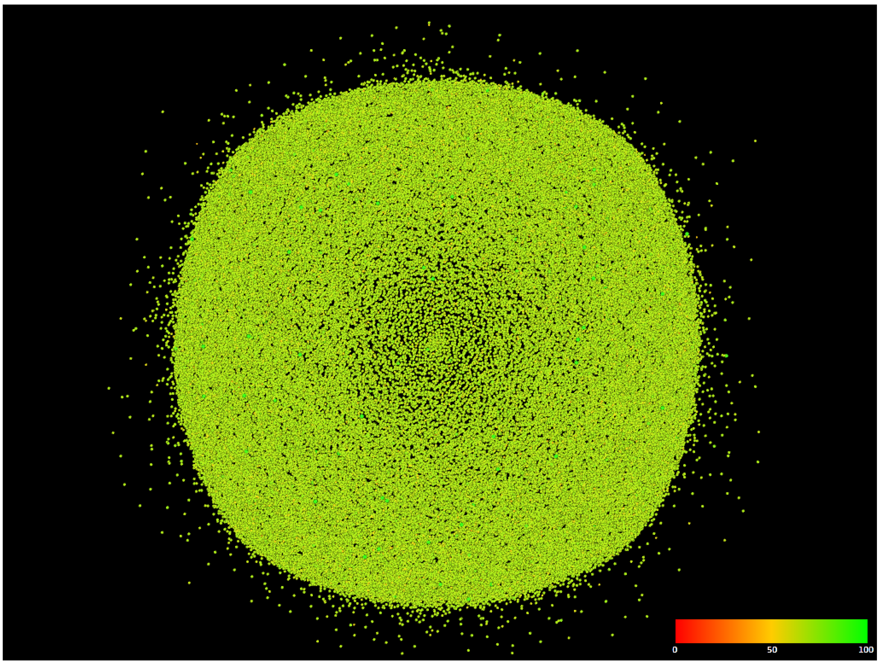
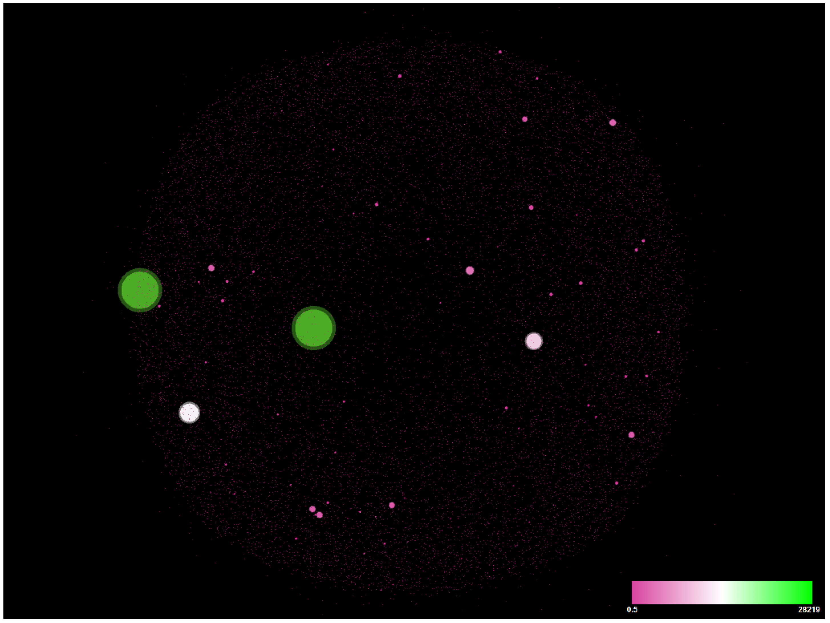
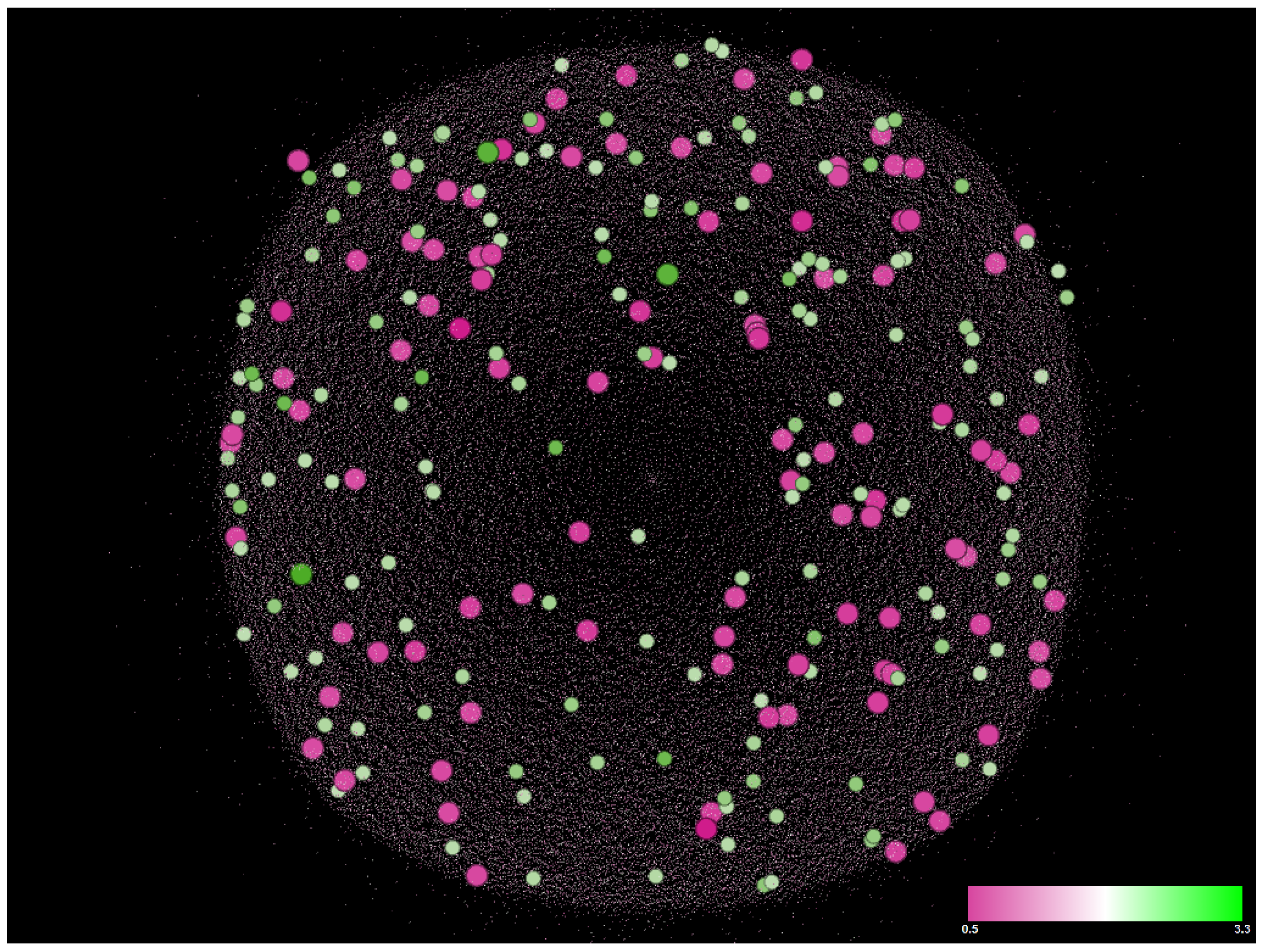
• 0% (red)—the router is always transmitting,
• 50% (yellow)—the router is transmitting for at least 50% of the time,
• 100% (green)—the router is never transmitting,
• between the above values, there are intermediate colors.

In the basic network, only 3.52% of the routers were idle and did not transmit for less than 25% of the time (

Table 3. Comparison of the number of nodes in an idle state (non-transmit) between the basic (B) and energy-saving (E) models.

State	Idle Time (%)	Nodes in N-Mode (%)	Nodes in ES-Mode (%)
Highly active	0–25	3.52	0.0024
Active	25–50	94.17	0.84
Mostly idle	50–75	2.31	99.15
Idle	75–100	0	0.006

). Most routers (94.17%) idled between 25% and 50% of the time, while only 2.31% of the nodes idled up to 75% of the time.

In energy-saving mode, the results have changed significantly. A tiny number of nodes (0.0024%) were in a non-transmitting state below 25% of the time. Only 0.84% of the routers idled up to 50% of the time. However, 99.15% of routers did not transmit up to 75% of the time. Some of them (0.006%) have never sent a packet (100% of the time).

We have additionally collected the idle time statistics for the most prolonged flow in the network (42 nodes) for the whole modeling period. The visualization in Figure 4 shows the difference of idle time between the two types of nodes, which varies between +18.8% and +40.6%.

The second set of results aims to determine the congestion rate. We proposed two indicators: $C{R}_{1i}$ and $C{R}_{2i}$. The first one is computed for any station i as the average of the ratios of queues $q_{e{s}_i}$ in the energy-aware network and queues $q_{n_i}$ in the basic network over the entire time, according to Equation (8), while the second is defined as the quotient of the average queues over the whole period, Equation (9). In both cases, we omitted the values where the queue lengths in the normal mode were zero.

$$C{R}_{1i}=\frac{1}{T}·\sum _{j=1}^T\frac{q_{e{s}_{i,j}}}{q_{n_{i,j}}},{\forall }_j{q}_{n_{i,j}}>0$$

(8)

$$C{R}_{2i}=\frac{\frac{1}{T}·{\sum }_{j=1}^T{q}_{e{s}_{i,j}}}{\frac{1}{T}·{\sum }_{j=1}^T{q}_{n_{i,j}}}.$$

(9)

The resulting $C{R}_{1i}$ rate ranged from 0.1876085 to 34,774.9. Thus, we decided to group them into six categories:

(a)

$C{R}_{1i}⩾\mathrm{10,000}$      circa 0.0048% of nodes,

(b)

$1000<C{R}_{1i}⩽\mathrm{10,000}$  circa 0.054% of nodes,

(c)

$100<C{R}_{1i}⩽1000$     circa 0.38% of nodes,

(d)

$10<C{R}_{1i}⩽100$      circa 4.9% of nodes,

(e)

$1<C{R}_{1i}⩽10$        circa 93.33% of nodes,

(f)

$C{R}_{1i}⩽1$           circa 1.33% of nodes.

Most of the values indicated that the congestion of a particular router was generally [1; 10] times greater (category e) in energy-saving mode than in normal mode (Figure 5). After further examination, the cases in category $\left(a\right)$ turned out to be routers with small buffers (18, 63, and 309 packets). In normal mode, the queue lengths at particular moments in time were practically null: at ${10}^{-6}$ level in the case of the 18-packet buffers and ${10}^{-4}$ for the 309 one, while the values in energy-saving mode exceeded the $T_B$ threshold (25%). The adopted colors in the figure represent the average number of times the congestion in the energy-saving network is greater than in the standard network:

• 0.558—violet,
• 14,110.012—white,
• 28,219.465—green,
• between the above values, there are intermediate colors.

The congestion rate ($C{R}_{1i}$) turns out to be very sensitive to transient spikes in the quotient values ($\frac{q_{e{s}_i}}{q_{n_i}}$). Sometimes even a single large value of quotient results in a huge increase in congestion rate $C{R}_{1i}$. Thus, we introduced another congestion rate of $C{R}_{2i}$, Equation (9), which allows a general comparison of queues in both modes.

The congestion rate $C{R}_{2i}$ illustrates how many times in the analyzed topology queues in the energy-saving mode are longer than the queues in normal mode. The extreme values we discover are 0.5714 and 3.3297, while for most nodes (99.7%) the changes are less significant—the indicator is in the range [0.75; 2.0]. The values are presented in Figure 6, where the values below 0.75 (violet) and above 2.0 (green) are enlarged.

The third set of results is focused on the identification of overload periods in the network nodes. The results are presented as functions of time within an interval of 100 s of a modeling session. Figure 7 and Figure 8 present, for standard and energy-saving models, as a function of time, the number of routers that have current queue lengths exceeding 20%, 25%, 50%, and 75% of the router buffer capacity. Figure 9 and Figure 10 present for both networks the time-dependent average percentage occupancy of all router buffers and the average throughput of the entire network. The energy-saving mode is seen to contribute to eliminating congestion periods and its performance is much smoother. However, the average throughput of connections in the energy-saving network is much lower, 4.49 (packet/s), than 8.31 (packet/s) in normal mode. If we queue packets and limit the transmission further, the bandwidth decreases. This is acceptable for non-priority traffic or for packets that do not have to meet the QoS conditions because it reduces the cost of electricity. Although for QoS traffic the decrease is too significant, thus the threshold parameters would have to be adjusted.

At the end, we give a few data on the model execution times. The computation, i.e., generation of both data sets using database procedures, was carried out in parallel for both models and took about 48 min (in the case of a toy 15-node network it was 20 s). Other times are not significant. The import of configuration data, including initial values, took 2 s per model, with 75% of the time to import the network structure. It should be noted that we have not focused on optimizing the time of data generation. The resulting data sets may be exploited, posing various inquiries, typically as several lines in SQL, precisely what type of results we need. The selection and export of data corresponding to the inquiries is generally below 1 s, e.g., extracting the data for idle period charts (Figure 3 and Figure 8) took 951 milliseconds; the export of the indicated data takes additionally several dozen milliseconds per file. It took a total of 2.3 s to generate all four data sets indicating overload moments (Figure 8). Calculations of CR1 (Figure 5) and CR2 (Figure 6) took 12.5 s and 3.6 s, respectively. It took 14 s and 3.8 s to determine the average buffer volume (Figure 9 and Figure 10, respectively.)

5. Conclusions

Queuing models, exploited for 100 years in performance evaluation of telecommunications systems and computer networks, usually refer to single nodes or small topologies. However, it is crucial to see the impact of various decisions, e.g., introducing new protocols or devices, on a much larger scale, corresponding to the size of the Internet.

In this article, we demonstrate that it is possible to formulate models which can analyze the performance of of very large network topologies. The use of fluid-flow approximation and the appropriate environment enables quantitative analysis based on the transient states of a network having more than one hundred thousand nodes and actual Internet topology, which is hierarchical and heterogeneous, with links and nodes of various capacities. A model of this size was never implemented before.

As the research of solutions minimizing the Internet’s energy consumption becomes an urgent issue, the model is used to investigate how the introduction of energy-saving on–off nodes influences the performance of the whole network. We see that it reduces network congestion and saves energy costs but significantly lowers network throughput. The approach tested here may facilitate various studies on large-scale networks.

In future work, we intend to investigate large topologies of the Internet of Things and Software Defined Networks. The Internet of Things and new services generate increasing traffic volumes and create new challenges for its transmission. Network structures based on static switches are not well suited to assure high performance, energy efficiency, and reliability in dynamically changing environments, and are not flexible enough to maintain Quality of Service for increasingly complex networks. SDN provides flexible and scalable routing, link failure recovery, load balancing, and security issues. As we have seen already with the use of diffusion approximation studying small SDN topologies, the SDN network is most of the time in a transient state due to frequent decisions of the controller [77,78]. Therefore, any optimization of its performance should be based on transient state modeling. The model presented here may reflect any network topology and time-dependent routing based on the decisions of the SDN controller, predicting the resulting transient behavior. Therefore, it is well suited to the performance evaluation of SDN networks and may be used for their optimization. We only need to define a goal function that combines QoS parameters such as transmission time, its variation, and loss probability with energy consumption.

References

1. Internet Growth Statistics. Available online: https://www.internetworldstats.com/emarketing.htm (accessed on 4 December 2021).
2. Data Centres and Data Transmission Networks, International Energy Agency Tracking Report, November 2021. Available online: https://www.iea.org/reports/data-centres-and-data-transmission-networks (accessed on 4 January 2021).
3. Berkeley Lab: It Takes 70 Billion Kilowatt Hours a Year to Run the Internet. Available online: https://www.forbes.com/sites/christopherhelman/2016/06/28/how-much-electricity-does-it-take-to-run-the-internet/?sh=7f7b4a261fff (accessed on 5 December 2021).
4. Jain, R. The Art of Computer Systems Performance Analysis: Techniques for Experimental Design, Measurement, Simulation and Modeling; Wiley: New York, NY, USA, 1991. [Google Scholar]
5. ns-2 Manual. Available online: http://nsnam.sourceforge.net/wiki/index.php/User_Information (accessed on 5 December 2021).
6. ns-3 Webpage. Available online: https://www.nsnam.org/ (accessed on 5 December 2021).
7. OPNeT++ Webpage. Available online: https://omnetpp.org/ (accessed on 5 December 2021).
8. Liu, Y.; Lo Presti, F.; Misra, V.; Towsley, D.; Gu, Y. Fluid Models and Solutions for Large-Scale IP Networks. In Proceedings of the 2003 ACM SIGMETRICS International Conference on Measurement and Modeling of Computer Systems, Association for Computing Machinery, SIGMETRICS ’03, San Diego, CA, USA, 9–14 June 2003; pp. 91–101. [Google Scholar] [CrossRef]
9. Misra, V.; Gong, W.B.; Towsley, D. Fluid-Based Analysis of a Network of AQM Routers Supporting TCP Flows with an Application to RED. In Proceedings of the Conference on Applications, Technologies, Architectures, and Protocols for Computer Communication. Association for Computing Machinery, SIGCOMM ’00, Stockholm, Sweden, 28 August–1 September 2000; pp. 151–160. [Google Scholar] [CrossRef]
10. Sakumoto, Y.; Ohsaki, H.; Imase, M. Design and Implementation of Flow-Level Simulator FSIM for Performance Evaluation of Large Scale Networks. Int. J. Comput. Sci. Telecommun. 2013, 4, 1–10. [Google Scholar]
11. Czachórski, T. Queuing models for performance evaluation of computer networks: Transient state analysis. In Analytic Methods in Interdisciplinary Applications; Mityushev, M.R.V., Ed.; Springer: Berlin, Germany, 2014; Volume 116, pp. 51–80. [Google Scholar] [CrossRef]
12. Erlang, A.K. The Theory of Probabilities and Telephone Conversations. Nyt Tidsskr. Mat. 1909, B20, 33–39. [Google Scholar]
13. Engset, T.O. Die Wahrscheinlichkeitsrechnung zur Bestimmung der Wahlerzahl in automatischen Fernsprechamtern. Elektrotechnische Z. 1918, 31, 304–306. [Google Scholar]
14. Domański, A.; Domańska, J.; Filus, K.; Szyguła, J.; Czachórski, T. Self-Similar Markovian Sources. Appl. Sci. 2020, 10, 3727. [Google Scholar] [CrossRef]
15. Czachórski, T.; Domańska, A.; Domańska, J.; Rataj, A. A Study of IP Router Queues with the Use of Markov Models. In International Conference on Computer Networks (CN2016); Springer: Cham, Switzerland, 2016; pp. 294–305. [Google Scholar] [CrossRef]
16. Stewart, W.J. An Introduction to the Numerical Solution of Markov Chains; Princeton University Press: Princeton, NJ, USA, 1994. [Google Scholar]
17. Kwiatkowska, M.; Norman, G.; Parker, D. PRISM 4.0: Verification of Probabilistic Real-time Systems. In Proceedings of the 23rd International Conference on Computer Aided Verification (CAV’11), Snowbird, UT, USA, 14–20 July 2011; pp. 585–591. [Google Scholar]
18. PRISM–Probabilistic Model Checker. Available online: http://www.prismmodelchecker.org (accessed on 4 December 2021).
19. Gelenbe, E. On Approximate Computer Systems Models. J. ACM 1975, 22, 261–269. [Google Scholar] [CrossRef]
20. Kobayashi, H. Modeling and Analysis: An Introduction to System Performance Evaluation Methodology; Addison-Wesley: Reading, MA, USA, 1978. [Google Scholar]
21. Czachórski, T. A method to solve diffusion equation with instantaneous return processes acting as boundary conditions. Bull. Pol. Acad. Sci. Tech. Sci. 1993, 41, 417–451. [Google Scholar]
22. Nycz, T.; Czachórski, T. Scalability study of computer network models using a diffusion approximation with an increase in the size of the modeled network. Stud. Inform. 2012, 33, 63–78. [Google Scholar]
23. Moran, P.A.P. A probability theory of dams and storage systems. Aust. J. Appl. Sci. 1954, 5, 116–124. [Google Scholar]
24. Nycz, T.; Nycz, M.; Czachórski, T. A numerical comparison of diffusion and fluid-flow approximations used in modelling transient states of TCP/IP networks. Computer Network. In Communications in Computer and Information Science; Springer: Berlin, Germnay, 2014; Volume 431, pp. 213–222. [Google Scholar]
25. Nycz, M.; Nycz, T.; Czachórski, T. Modelling Dynamics of TCP Flows in Very Large Network Topologies. In Information Sciences and Systems 2015; Lecture Notes in Electrical Engineering; Springer: Cham, Swizerland, 2016; Volume 363. [Google Scholar] [CrossRef]
26. Nycz, M.; Nycz, T.; Czachórski, T. Performance modelling of transmissions in very large network topologies. In International Conference on Distributed Computer and Communication Networks; Distributed Computer and Communication Networks; Springer: Moscow, Russia, 2017; Volume 700, pp. 49–62. [Google Scholar]
27. Czachórski, T.; Nycz, M.; Nycz, T. Fluid-Flow Approximation using ETL Process and SAP HANA Platform. In HPI Future SOC Lab: Proceedings 2016; Universität Potsdam: Potsdam, Germany, 2018; pp. 63–66. [Google Scholar]
28. Nycz, M. Modeling of Computer Networks Using SAP HANA Smart Data Streaming. In International Conference on Computer Networks; Communications in Computer and Information Science; Springer: Berlin, Germany, 2019; Volume 1039, pp. 48–61. [Google Scholar]
29. Lyon, B. The Opte Project. Available online: http://www.opte.org/ (accessed on 5 December 2021).
30. Alam, T. A Reliable Communication Framework and Its Use in Internet of Things (IoT). Int. J. Sci. Res. Comput. Sci. Eng. Inf. Technol. 2018, 3, 450–456. [Google Scholar]
31. Kanoun, O.; Bradai, S.; Khriji, S.; Bouattour, G.; El Houssaini, D.; Ben Ammar, M.; Naifar, S.; Bouhamed, A.; Derbel, F.; Viehweger, C. Energy-Aware System Design for Autonomous Wireless Sensor Nodes: A Comprehensive Review. Sensors 2021, 21, 548. [Google Scholar] [CrossRef] [PubMed]
32. Panda, N.; Sahu, P.K.; Parhi, M.; Pattanayak, B.K. A Survey on Energy Awareness Mechanisms in ACO-Based Routing Protocols for MANETs. In Intelligent and Cloud Computing. Smart Innovation, Systems and Technologie; Springer: Berlin, Germany, 2021; Volume 194. [Google Scholar] [CrossRef]
33. Barker, A.; Swany, M. Energy Aware Routing with Computational Offloading for Wireless Sensor Networks. arXiv 2020, arXiv:2011.14795. [Google Scholar]
34. Chaurasia, N.; Kumar, M.; Chaudhry, R.; Verma, O.P. Comprehensive survey on energy-aware server consolidation techniques in cloud computing. J. Supercomput. 2021, 50, 1–56. [Google Scholar] [CrossRef]
35. Fonseca, A.; Kazman, R.; Lago, P. A Manifesto for Energy-Aware Software. IEEE Softw. 2019, 36, 79–82. [Google Scholar] [CrossRef]
36. Beyer, D.; Wendler, P. CPU Energy Meter: A Tool for Energy-Aware Algorithms Engineering. In Tools and Algorithms for the Construction and Analysis of Systems. TACAS 2020; Lecture Notes in Computer Science; Springer: Berlin, Germany, 2020; Volume 12079, pp. 126–133. [Google Scholar] [CrossRef] [Green Version]
37. Gallersdörfer, U.; Klaaßen, L.; Stoll, C. Energy Consumption of Cryptocurrencies Beyond Bitcoin. Joule 2020, 4, 1843–1846. [Google Scholar] [CrossRef]
38. Zhang, Q.; Lin, X.; Hao, Y.; Cao, J. Energy-Aware Scheduling in Edge Computing Based on Energy Internet. IEEE Access 2020, 8, 229052–229065. [Google Scholar] [CrossRef]
39. Hao, Y.; Cao, J.; Wang, Q.; Du, J. Energy-aware scheduling in edge computing with a clustering method. Future Gener. Comput. Syst. 2021, 117, 259–272. [Google Scholar] [CrossRef]
40. Mao, J.; Cao, T.; Peng, X.; Bhattacharya, T.; Ku, W.S.; Qin, X. Security-Aware Energy Management in Clouds. In Proceedings of the 2020 Second IEEE International Conference on Trust, Privacy and Security in Intelligent Systems and Applications (TPS-ISA), Atlanta, GA, USA, 28–31 October 2020; pp. 284–293. [Google Scholar] [CrossRef]
41. Mishra, S.K.; Mishra, S.; Alsayat, A.; Jhanjhi, N.Z.; Humayun, M.; Sahoo, K.S.; Luhach, A.K. Energy-Aware Task Allocation for Multi-Cloud Networks. IEEE Access 2020, 8, 178825–178834. [Google Scholar] [CrossRef]
42. Chen, X.; Tan, T.; Cao, G.; La Porta, T.F. Energy-Aware and Context-Aware Video Streaming on Smartphones. In Proceedings of the 2019 IEEE 39th International Conference on Distributed Computing Systems (ICDCS), Dallas, TX, USA, 7–10 July 2019. [Google Scholar] [CrossRef]
43. Wheatman, K.; Mehmeti, F.; Mahon, M.; La Porta, T.; Cao, G. Multi-User Competitive Energy-Aware and QoE-Aware Video Streaming on Mobile Devices. In Proceedings of the 16th ACM Symposium on QoS and Security for Wireless and Mobile Networks, Q2SWinet ’20, Alicante, Spain, 16–20 November 2020; Association for Computing Machinery: New York, NY, USA, 2020; pp. 47–55. [Google Scholar] [CrossRef]
44. Alhasan, A.; Audah, L.; Alwan, M.H.; Alobaidi, O.R. AN Energy Aware QoS Trust Model for Energy Consumption Enhancement Based on Cluster for IoT Networks. J. Eng. Sci. Technol. 2021, 16, 957–976. [Google Scholar]
45. Mujeeb, S.M.; Sam, R.P.; Madhavi, K. Trust and energy aware routing algorithm for Internet of Things networks. Int. J. Numer. Model. Electron. Netw. Devices Fields 2021, 34, e2858. [Google Scholar] [CrossRef]
46. Khaleghnasab, R.; Bagherifard, K.; Ravaei, B.; Parvin, H.; Nejatian, S. An Energy and Load Aware Multipath Routing Protocol in the Internet of Things. Preprints 2020. [Google Scholar] [CrossRef]
47. Bolla, R.; Bruschi, R.; Chiappero, M.; D’Agostino, L.; Lago, P.; Lombardo, C.; Mangialardi, S.; Podda, F. EE-DROP: An energy-aware router prototype. In Proceedings of the 2013 24th Tyrrhenian International Workshop on Digital Communications-Green ICT (TIWDC), Genoa, Italy, 23–25 September 2013; pp. 1–6. [Google Scholar] [CrossRef]
48. Bolla, R.; Bruschi, R.; Ortiz, O.M.J.; Lago, P. An Experimental Evaluation of the TCP Energy Consumption. IEEE J. Sel. Areas Commun. 2015, 33, 2761–2773. [Google Scholar] [CrossRef]
49. Bruschi, R.; Lombardo, A.; Panarello, C.; Podda, F.; Santagati, E.; Schembra, G. Active window management: Reducing energy consumption of TCP congestion control. In Proceedings of the 2013 IEEE International Conference on Communications (ICC), Budapest, Hungary, 9–13 June 2013; pp. 4154–4158. [Google Scholar] [CrossRef]
50. Kim, T.; Lee, J.; Cha, H.; Ha, R. An energy-aware transmission mechanism for wifi-based mobile devices handling upload TCP traffic. Int. J. Commun. Syst. 2009, 22, 625–640. [Google Scholar] [CrossRef]
51. Wu, Y.; Yang, Q.; Li, H.; Kwak, K.S.; Leung, V.C.M. Control-Aware Energy-Efficient Transmissions for Wireless Control Systems with Short Packets. IEEE Internet Things J. 2021, 8, 14920–14933. [Google Scholar] [CrossRef]
52. Oulmahdi, M.; Chassot, C.; Exposito, E. An Energy-Aware TCP for Multimedia Streaming. In Proceedings of the 2013 International Conference on Smart Communications in Network Technologies (SaCoNeT), Paris, France, 17–19 June 2013; Volume 1, pp. 1–5. [Google Scholar] [CrossRef]
53. Le, T.A.; Hong, C.S.; Razzaque, M.A.; Lee, S.; Jung, H. ecMTCP: An Energy-Aware Congestion Control Algorithm for Multipath TCP. IEEE Commun. Lett. 2012, 16, 275–277. [Google Scholar] [CrossRef]
54. Lim, Y.S.; Chen, Y.C.; Nahum, E.M.; Towsley, D.; Gibbens, R.J.; Cecchet, E. Design, Implementation, and Evaluation of Energy-Aware Multi-Path TCP. In Proceedings of the 11th ACM Conference on Emerging Networking Experiments and Technologies, CoNEXT ’15, Heidelberg, Germany, 1–4 December 2015; Association for Computing Machinery: New York, NY, USA, 2015. [Google Scholar] [CrossRef]
55. Zhao, J.; Liu, J.; Wang, H. On Energy-Efficient Congestion Control for Multipath TCP. In Proceedings of the 2017 IEEE 37th International Conference on Distributed Computing Systems (ICDCS), Atlanta, GA, USA, 5–8 June 2017; pp. 351–360. [Google Scholar] [CrossRef]
56. Sheeba, G.M. Energy Aware Router Placements Using Fuzzy Differential Evolution. In Wireless Mesh Networks-Security, Architectures and Protocols; IntechOpen: London, UK, 2019. [Google Scholar] [CrossRef] [Green Version]
57. Chen, Y.; Das, A.; Qin, W.; Sivasubramaniam, A.; Wang, Q.; Gautam, N. Managing Server Energy and Operational Costs in Hosting Centers. In Proceedings of the 2005 ACM SIGMETRICS International Conference on Measurement and Modeling of Computer Systems. Association for Computing Machinery, SIGMETRICS ’05, Coimbra, Portugal, 12–14 July 2005; pp. 303–314. [Google Scholar] [CrossRef] [Green Version]
58. Maccio, V.J.; Down, D.G. Exact Analysis of Energy-Aware Multiserver Queueing Systems with Setup Times. In Proceedings of the 2016 IEEE 24th International Symposium on Modeling, Analysis and Simulation of Computer and Telecommunication Systems (MASCOTS), London, UK, 19–21 September 2016; pp. 11–20. [Google Scholar] [CrossRef]
59. Deiana, E.; Latouche, G.; Remiche, M.A. Fluid Flow Model for Energy-Aware Server Performance Evaluation. SIGMETRICS Perform. Eval. Rev. 2018, 45, 204–209. [Google Scholar] [CrossRef]
60. Lu, X. Energy-aware Performance Analysis of Queueing Systems. Master’s Thesis, School of Electrical Engineering, Aalto University, Espoo, Finland, 2013. [Google Scholar]
61. Gebrehiwot, M.E.; Aalto, S.; Lassila, P. Optimal sleep-state control of energy-aware M/G/1 queues. EAI Endorsed Trans. Internet Things 2015, 1, e5. [Google Scholar] [CrossRef] [Green Version]
62. Narman, H.S.; Atiquzzaman, M. Energy aware scheduling and queue management for next generation Wi-Fi routers. In Proceedings of the 2015 IEEE Wireless Communications and Networking Conference Workshops (WCNCW), New Orleans, LA, USA, 9–12 March 2015; pp. 148–152. [Google Scholar] [CrossRef]
63. Barbera, M.; Lombardo, A.; Schembra, G. A fluid-based model of time-limited TCP flows. Comput. Netw. 2004, 44, 275–288. [Google Scholar] [CrossRef] [Green Version]
64. Abdeljaouad, I.; Rachidi, H.; Fernandes, S.; Karmouch, A. Performance analysis of modern TCP variants: A comparison of Cubic, Compound and New Reno. In Proceedings of the 2010 25th Biennial Symposium on Communications, Kingston, ON, Canada, 12–14 May 2010; pp. 80–83. [Google Scholar] [CrossRef]
65. Alam, M.J.; Chowdhury, T. Performance Evaluation of TCP Vegas over TCP Reno and TCP New Reno over TCP Reno. Int. J. Inform. Vis. 2019, 3, 275–282. [Google Scholar]
66. Saedi, T.; El-Ocla, H. TCP CERL+: Revisiting TCP congestion control in wireless networks with random loss. Wirel. Netw. 2021, 27, 423–440. [Google Scholar] [CrossRef]
67. Mohamed, K.; Hussein, S.; Abdi, A.; Seddiq, A.E. Studying the TCP Flow and Congestion Control Mechanisms Impact on Internet Environment. Int. J. Comput. Sci. Inf. Secur. 2018, 16, 174–179. [Google Scholar]
68. Kanagarathinam, M.R.; Singh, S.; Sandeep, I.; Kim, H.; Maheshwari, M.K.; Hwang, J.; Roy, A.; Saxena, N. NexGen D-TCP: Next Generation Dynamic TCP Congestion Control Algorithm. IEEE Access 2020, 8, 164482–164496. [Google Scholar] [CrossRef]
69. Braden, B.; Clark, D.; Crowcroft, J.; Davie, B.; Deering, S.; Estrin, D.; Floyd, S.; Jacobson, V.; Minshall, G.; Partridge, C.; et al. Recommendations on Queue Management and Congestion Avoidance in the Internet. RFC 2309, IETF. 1998. Available online: https://datatracker.ietf.org/doc/html/rfc2309 (accessed on 13 December 2021).
70. Floyd, S.; Jacobson, V. Random early detection gateways for congestion avoidance. IEEE/ACM Trans. Netw. 1993, 1, 397–413. [Google Scholar] [CrossRef]
71. Nycz, M.; Czachórski, T. Modelowanie dynamiki natężenia przesyłów TCP/IP. In Zastosowania Internetu; Pikiewicz, P., Ed.; Wydawnictwo WSB w: Dąbrowie Górniczej, Poland, 2012. [Google Scholar]
72. Fluid Flow Analysis of RED Algorithm with Modified Weighted Moving Average. In Modern Probabilistic Methods for Analysis of Telecommunication Networks. BWWQT 2013; Communications in Computer and Information Science; Springer: Berlin/Heidelberg, Germnay, 2013; Volume 356, pp. 50–58. [CrossRef]
73. SAP HANA Platform. Available online: https://www.sap.com/products/hana.html (accessed on 4 January 2021).
74. Gnuplot-Graphing Utility. Available online: http://www.gnuplot.info/ (accessed on 5 December 2021).
75. Gephi: The Open Graph Viz Platform. Available online: http://gephi.github.io/ (accessed on 5 December 2021).
76. Nycz, M.; Nycz, T.; Czachórski, T. An Analysis of the Extracted Parts of Opte Internet Topology. In Computer Networks, CN 2015; Communications in Computer and Information Science; Springer: Cham, Switzerland, 2015; Volume 522. [Google Scholar] [CrossRef]
77. Czachórski, T.; Gelenbe, E.; Kuaban, G.S.; Marek, D. Time-Dependent Performance of a Multi-Hop Software Defined Network. Appl. Sci. 2021, 11, 2469. [Google Scholar] [CrossRef]
78. Nycz, T.; Czachórski, T.; Nycz, M. Diffusion Model of Preemptive-Resume Priority Systems and Its Application to Performance Evaluation of SDN Switches. Sensors 2021, 21, 5024. [Google Scholar] [CrossRef] [PubMed]
Figure 1. Database schema for numerical calculation.
Mathematics 09 03279 g001
Figure 2. Idle times per router, basic model.
Mathematics 09 03279 g002
Figure 3. Idle times per router, energy-aware model.
Mathematics 09 03279 g003
Figure 4. Comparison of the idle times in the longest flow, basic and energy-aware models. The horizontal axis displays the unique numbers of network nodes that form the path of the flow.
Mathematics 09 03279 g004
Figure 5. Congestion rate ( C R 1 i ) in the network.
Mathematics 09 03279 g005
Figure 6. Congestion rate ( C R 2 i ) in the network.
Mathematics 09 03279 g006
Figure 7. The number of routers having current queue lengths greater than 20% and 25% of their buffer sizes in basic and energy-saving models.
Mathematics 09 03279 g007
Figure 8. The number of routers having the current queue length ⩾50% and 75% of the buffer for basic and energy-saving models. The curves for energy-saving mode are close to zero and practically invisible on the linear scale.
Mathematics 09 03279 g008
Figure 9. Average occupancy of router queues (percentage of buffer volume) as a function of time for basic and energy-saving models.
Mathematics 09 03279 g009
Figure 10. Average throughput per link in the network as a function of time for basic and energy-saving models.
Mathematics 09 03279 g010