Performance Evaluation of the Priority Multi-Server System MMAP/PH/M/N Using Machine Learning Methods

Abstract

In this paper, we present the results of a study of a priority multi-server queuing system with heterogeneous customers arriving according to a marked Markovian arrival process (MMAP), phase-type service times (PH), and a queue with finite capacity. Priority traffic classes differ in PH distributions of the service time and the probability of joining the queue, which depends on the current length of the queue. If the queue is full, the customer does not enter the system. An analytical model has been developed and studied for a particular case of a queueing system with two priority classes. We present an algorithm for calculating stationary probabilities of the system state, loss probabilities, the average number of customers in the queue, and other performance characteristics for this particular case. For the general case with K priority classes, a new method for assessing the performance characteristics of complex priority systems has been developed, based on a combination of machine learning and simulation methods. We demonstrate the high efficiency of the new method by providing numerical examples.

1. Introduction

Priority queuing systems, which are an essential part of the queuing theory, are effectively used in the analysis of real technical and social systems [1,2,3,4,5,6,7]. Examples of systems with priority traffic include digital television, in which the transmission of synchronization signals has a higher priority than the transmission of video, and computer networks with Quality of Service (QoS) support, in particular—Internet of Things (IoT) systems [1,2,3,4]. Furthermore, information services with different categories of users [5], as well as any social systems with different types of clients, such as hospitals, are other examples of the systems with priority traffic. As an example of the latter, we can cite the studies [6,7], which investigate the effectiveness of algorithms for allocating places in the organ transplant queue for patients depending on the severity of their disease. In addition, priority systems are used to provide users with priority login when working with various services. For example, the paper [5] provides an analysis of the impact of priorities on the workload, transaction time, and other characteristics, investigating the performance of various databases for users with different access priorities.

It is well-known [8] that traffic in modern computer networks is correlated, and it is essential to use Markovian arrival processes ($MAP$) [9] to model it. A natural generalization of $MAP$ for the case of heterogeneous traffic is marked Markovian arrival process (Marked $MAP$, $MMAP$) [9], which describes correlated arrivals of an arbitrary number of customers types.

Systems with $MMAP$ are poorly studied in the world literature compared to classical $MAP$ arrival processes. The article [10] analyzes the queue size of the priority system $MMAP/MAP/1$. Investigation of the conditions for a stationary mode of a multi-server queueing system with an incoming $MMAP$ is presented in the paper [6]. However, it lacks a description of the algorithm for calculating stationary state probabilities and other system performance characteristics. In recent works [11,12], the problem of finding a stationary solution for priority systems with a $MMAP$ for the case of one server was investigated. The paper [11] examines the relative priority queue, and [12] examines the absolute priority queue.

Paper [13] considers a complex multi-server queueing system with a $MMAP$, two priority classes, and no buffer. Current research is a development and generalization of this paper. The fundamental difference between this paper and [13] is the presence of a buffer of finite capacity and an arbitrary number of customers types. On the one hand, such a generalization significantly complicates the mathematical analysis even for two customers types. However, on the other hand, it expands the area of the practical application of the model considered in the paper. The key contribution of this research is the development of a new method for studying queueing systems with an arbitrary number of customers types, based on a combination of machine learning and simulation methods. This method can be effectively used to study many problems in the theory of queues, for which finding a rigorous analytical solution and numerical results is either difficult or even impossible using traditional approaches. In particular, this method was applied to study a Fork-join type QS, and in [14] to estimate performance characteristics of complex adaptive polling systems.

This paper presents for the first time the results of a study of a multi-server queueing system with a $MMAP$, a queue with finite capacity, and an arbitrary number of customers types. The service times for customers of all types have a phase-type ($PH$) distribution with different parameters. Section 2 provides the formal problem statement and description of the model. For a particular case of two types of customers, Section 3 gives an analytical solution, including a description of a multidimensional Markov chain, an algorithm for calculating stationary state probabilities, and other characteristics. Section 4 describes a new method for studying a generalized model of a multi-server queueing system based on a combination of machine learning and simulation methods. Finally, Section 5, using a new approach, presents the results of a numerical study of the crucial characteristics of the multi-server queueing system, including the loss probabilities of the customers and the time spent by customers of the given type in the system. Section 6 discusses results and concludes the paper.

2. Problem Statement

Let us consider a multi-server queueing system with N servers and a queue with capacity R. Customers of different types arrive according to a marked Markovian arrival process directed by the underlying irreducible continuous time Markov chain ${\nu }_t$, $t\ge 0$ with state space $\{0,1,2,\dots ,W\}$. Process ${\nu }_t$ stays in state $\nu$ during exponentialy distributed time with parameter ${\lambda }_{\nu }$, $\nu =\overline{0,W}$. After that the process moves to state ${\nu }^{\prime }$ and either generates a customer of type k, $k\in \{1,2,\dots ,K\}$ with probability $p_k(\nu ,{\nu }^{\prime })$, or moves without customer generation with probability $p_0(\nu ,{\nu }^{\prime })$. Any possible loop transition should happen together with customer generation, i.e., $p_k(\nu ,\nu )\ge 0$, $k\in \{1,2,\dots ,K\}$, but $p_0(\nu ,\nu )=0$. Transition probabilities should meet the following requirement:

$${\displaystyle \sum _{k=0}^K}{\displaystyle \sum _{{\nu }^{\prime }=0}^W}{p}_k(\nu ,{\nu }^{\prime })=1, \nu ,{\nu }^{\prime }=\overline{0,W}.$$

Thus, the $MMAP$ process is defined by

• $W+1$, number of states in the underlying Markov chain;
• K, number of customer types;
• ${\lambda }_{\nu }$, transition rates;
• $p_k(\nu ,{\nu }^{\prime })$, $k=\overline{0,K}$, $\nu ,{\nu }^{\prime }=\overline{0,W}$, transition probabilities between states in the underlying Markov chain ${\nu }_t$.

All the information regarding $MMAP$ process is conveniently stored in square matrices $D_k$, $k=\overline{0,K}$ of order $W+1$:

$$\begin{array}{cc}\hfill {\left(D_k\right)}_{\nu ,{\nu }^{\prime }}& ={\lambda }_{\nu }{p}_k(\nu ,{\nu }^{\prime }),\hspace{1em} \nu ,{\nu }^{\prime }=\overline{0,W},k=\overline{1,K},\hfill \\ \hfill {\left(D_0\right)}_{\nu ,{\nu }^{\prime }}& =\left\{\begin{array}{cc}-{\lambda }_{\nu },\hfill & \nu ={\nu }^{\prime }=\overline{0,W},\hfill \\ {\lambda }_{\nu }{p}_0(\nu ,{\nu }^{\prime }),\hfill & \nu \ne {\nu }^{\prime },\nu ,{\nu }^{\prime }=\overline{0,W}.\hfill \end{array}\right.\hfill \end{array}$$

Elements of matrices $D_k$, $k=\overline{1,K},$ are transitions rates of the process ${\nu }_t$, accompanied by generation of type k customers. Non-diagonal elements of matrix $D_0$ have a similar meaning, while diagonal elements hold the negated sum of state departure transition rates.

A natural requirement for the matrices $D_k$, $k=\overline{1,K},$ is that not all of them are zero. When this requirement is met, the matrix $D_0$ is non-degenerate and stable since its eigenvalues have a negative real part.

The matrices $D_k$, $k=\overline{1,K},$ can be defined by their matrix generating function $D\left(z\right)={\displaystyle \sum _{k=0}^K}{D}_k{z}^k, \left|z\right|<1.$ Note that the value of this function at $z=1$ (matrix $D\left(1\right)$) is the infinitesimal generator of the underlying Markov chain ${\nu }_t$, $t\ge 0$. The stationary distribution of this chain, represented as a rowvector $\mathit{\theta }$, is defined as a solution of the linear algebraic system $\mathit{\theta }D\left(1\right)=0, \mathit{\theta }\mathbf{e}=1.$ Here and below $\mathbf{e}$ is a column vector consisting of ones.

Arrival rate ${\lambda }_k$ of customers of type k and the total cumulative arrival rate $\lambda$ of $MMAP$ process are defined as

$$\begin{array}{cc}\hfill {\lambda }_k& =\mathit{\theta }{D}_k\mathbf{e},k=\overline{1,K}\hfill \\ \hfill \lambda & =\mathit{\theta }{\displaystyle \sum _{k=1}^K}{D}_k\mathbf{e}.\hfill \end{array}$$

Variance $v_k$ of inter-arrival intervals of k-type customers is calculated as

$$v^{\left(k\right)}=\frac{2\mathit{\theta }{(-D_0-{\displaystyle \sum _{l=1,l\ne k}^K}{D}_l)}^{-1}\mathbf{e}}{{\lambda }_k}-{\left(\frac{1}{{\lambda }_k}\right)}^2, k=\overline{1,K}.$$

Correlation coefficient $c_{cor}^{\left(k\right)}$ of lengths of two adjacent inter-arrival intervals of k-type customers is calculated by the formula

$$c_{cor}^{\left(k\right)}=[\frac{\mathit{\theta }{(D_0+{\displaystyle \sum _{l=1,l\ne k}^K}{D}_l)}^{-1}\mathbf{e}}{{\lambda }_k}{D}_k{(D_0+{\displaystyle \sum _{l=1,l\ne k}^K}{D}_l)}^{-1}\mathbf{e}-{\left(\frac{1}{{\lambda }_k}\right)}^2]v_k^{-1}, k=\overline{1,K}.$$

More details about a $MMAP$ can be found, for instance, in [15]. Note that stationary Poisson arrival process is a special case of $MMAP$ with $W=0$, $K=1$, $D_0=-\lambda$ and $D_1=\lambda$.

In the general case, customers of different types differ in priorities and parameters of $PH$ distribution of service time. These differences will be described in more detail below.

Let us consider that all servers are equal and operate independently. Service time of the k-type customer has $PH$ (Phase Type) distribution with representation $({\mathit{\beta }}_k,S_k)$. Here ${\mathit{\beta }}_k$ is a row vector of size $M_k$, and $S_k$ is a square matrix of size $M_k$. Thus, the service time is interpreted as the time during which an underlying Markov chain $m_t^{\left(k\right)}$, $t\ge 0,$ with state space $\{1,\dots ,M_k,M_k+1\}$, will reach the only absorbing state $M_k+1$. Transition rates of the chain $m_t^{\left(k\right)}$, $t\ge 0,$ within the space of transient states $\{1,\dots ,M_k\}$ are defined by the sub-generator $S_k,$ and the transition rates to the absorbing state are defined by the vector ${\mathit{S}}_0^{\left(k\right)}=-S_k\mathbf{e}$. Initial state of the process $m_t\left(k\right)$, $t\ge 0,$ at the time the service starts is selected according to the probability row vector ${\mathit{\beta }}_k$. More information regarding PH distributions may be found, e.g., in [16,17].

We assume that customers of type $k^{\prime }<k$ have higher relative priority than customers of type k. It means that all customers with higher priority are placed in the queue in front of customers with lower priority. Let an incoming customer of type $k^{\prime }$ finds all servers busy and $i=\overline{1,R-1}$, customers waiting in the queue. With probability $q_i^{\left(k^{\prime }\right)}$ this customer will join the queue and will be put ahead of all non-priority customers of types $k=k^{\prime }+1,k^{\prime }+2,\dots ,K$ and after all priority customers of types $k=1,2,\dots ,k^{\prime }$. With probability $1-q_i^{\left(k^{\prime }\right)}$, the new customer decides not to join the queue and leaves the system forever. If any new customer finds the queue fully occupied, it also leaves the system forever. To simplify notation, in the case of $K=2$ types of customers, we will denote the probabilities of joining the queue of length i for priority customers of type $k=1$ as $q_i\equiv q_i^{\left(1\right)}$, and for non-priority customers of type $k=2$ as $f_i\equiv q_i^{\left(2\right)}$.

Our goal is to calculate the stationary distribution of the system, its performance characteristics and conduct a numerical experiment to measure performance, including the probability of customers losses and the system’s response time. We will use the analytic model, Monte Carlo method, and machine learning (ML) to calculate the system characteristics.

3. $\mathit{M}\mathit{M}\mathit{A}\mathit{P}/\mathit{P}\mathit{H}/\mathit{M}/\mathit{N}$ Queueing System with Two Priority Classes

3.1. Markov Chain of the System States

Let at the time t,

• $i_t$ be the number of customers in the queue, $i_t=\overline{0,R}$;
• $k_t$ be the number of high priority (type 1) customers in the queue, $k_t=\overline{0,i_t}$;
• $n_t$ be the number of busy servers, $n_t=\overline{0,N}$;
• $r_t$ be the number of servers servicing high priority customers, $r_t=\overline{0,n_t}$;
• $n_t^{\left(m_t^{\left(1\right)}\right)}$ be the number of servers servicing high priority customers for which the underlying process is in state $m_t^{\left(1\right)}$, $n_t^{\left(m_t^{\left(1\right)}\right)}=\overline{0,r_t},$ $m_t^{\left(1\right)}=\overline{1,M_1}$;
• ${\tilde{n}}_t^{\left(m_t^{\left(2\right)}\right)}$ be the number of servers servicing low priority (type 2) customers for which the underlying process is in state $m_t^{\left(2\right)}$, ${\tilde{n}}_t^{\left(m_t^{\left(2\right)}\right)}=\overline{0,n_t-r_t},$ $m_t^{\left(2\right)}=\overline{1,M_2}$;
• ${\nu }_t$ be the state of the underlying process of $MMAP$, ${\nu }_t=\overline{0,W}$.

Operation of the system is described by a regular irreducible Markov chain ${\xi }_t$ with continuous time

$${\xi }_t=\{(i_t,k_t,r_t,n_t,{\nu }_t,n_t^{\left(1\right)},n_t^{\left(2\right)},\dots ,n_t^{\left(M_1\right)},{\tilde{n}}_t^{\left(1\right)},{\tilde{n}}_t^{\left(2\right)},\dots ,{\tilde{n}}_t^{\left(M_2\right)}), t\ge 0\},$$

with the state space

$$\begin{array}{c}\Omega =\{(i,n,r,\nu ,n^{\left(1\right)},n^{\left(2\right)},\dots ,n^{\left(M_1\right)},{\tilde{n}}^{\left(1\right)},{\tilde{n}}^{\left(2\right)},\dots ,{\tilde{n}}^{\left(M_2\right)}),\\ i=0, n=\overline{0,N}, r=\overline{0,n}, \nu =\overline{0,W}, n^{\left(m\right)}=\overline{0,r}, m=\overline{1,M_1}, {\tilde{n}}^{\left(\tilde{m}\right)}=\overline{0,n-r}, \tilde{m}=\overline{1,M_2}\} \bigcup \end{array}$$

$$\{(i,k,n,r,\nu ,n^{\left(1\right)},n^{\left(2\right)},\dots ,n^{\left(M_1\right)},{\tilde{n}}^{\left(1\right)},{\tilde{n}}^{\left(2\right)},\dots ,{\tilde{n}}^{\left(M_2\right)}),$$

$$\begin{array}{c}i=\overline{1,R}, k=\overline{0,i}, n=N, r=\overline{0,n}, \nu =\overline{0,W}, n^{\left(m^{\left(1\right)}\right)}=\overline{0,r}, m^{\left(1\right)}=\overline{1,M_1}, {\tilde{n}}^{\left(m^{\left(1\right)}\right)}=\overline{0,N-r},\\ m^{\left(2\right)}=\overline{1,M_2}, {\displaystyle \sum _{m^{\left(1\right)}=1}^{M_1}}{n}^{\left(m^{\left(1\right)}\right)}=r, {\displaystyle \sum _{m^{\left(2\right)}=1}^{M_2}}{\tilde{n}}^{\left(m^{\left(2\right)}\right)}=N-r.\}\end{array}$$

The number of vectors in the state space for $i=0$ is

$$K_0=(W+1){\displaystyle \sum _{n=0}^N}{\displaystyle \sum _{r=0}^n}{C}_{r+M_1-1}^{M_1-1}{C}_{n-r+M_2-1}^{M_2-1},$$

and, for any fixed $i=\overline{1,R},$ the number of vectors is

$$K=(i+1)(W+1){\displaystyle \sum _{r=0}^N}{C}_{r+M_1-1}^{M_1-1}{C}_{N-r+M_2-1}^{M_2-1}.$$

Let us denote:

• I (O) is an identity (zero) matrix of the appropriate dimension;
• $\overline{W}=W+1;$
• ⊗ and ⊕ are the symbols of the Kronecker product and sum of matrices, see [18];
• $C_n^l=\frac{n!}{l!(n-l)!}$;
• $d_r^{\left(1\right)}=C_{r+M_1-1}^{M_1-1}$;
• $d_r^{\left(2\right)}=C_{r+M_2-1}^{M_2-1}$;
• $diag\{a_1,a_2,\cdots ,a_n\}$ is a block diagonal matrix in which the diagonal blocks are $a_i$, $i=\overline{1,n}$, and the remaining blocks are zero;
• $dia{g}^{+}\{a_1,a_2,\cdots ,a_n\}$ is a square over-diagonal block matrix in which the over-diagonal blocks are $a_i$, $i=\overline{1,n}$, and the remaining blocks are zero, i.e., this is a matrix of the form

  $$\left(\begin{array}{cccccc}0& a_1& 0& \dots & 0& 0\\ 0& 0& a_2& \dots & 0& 0\\ ⋮& ⋮& ⋮& \ddots & ⋮& ⋮\\ 0& 0& 0& \dots & 0& a_n\\ 0& 0& 0& \dots & 0& 0\end{array}\right);$$
• $dia{g}^{-}\{a_1,a_2,\cdots ,a_n\}$ is a square sub-diagonal block matrix in which the sub-diagonal blocks are $a_i$, $i=\overline{1,n}$, and the remaining blocks are zero, i.e., this is a matrix of the form

  $$\left(\begin{array}{cccccc}0& 0& 0& \dots & 0& 0\\ a_1& 0& 0& \dots & 0& 0\\ 0& a_2& 0& \dots & 0& 0\\ ⋮& ⋮& ⋮& \ddots & ⋮& ⋮\\ 0& 0& 0& \dots & a_n& 0\end{array}\right);$$
• ${\overline{q}}_i=1-q_i,{\overline{f}}_i=1-f_i$;
• ${\mathbf{n}}_t^{\left(1\right)}=\{n_t^{\left(1\right)},n_t^{\left(2\right)},\dots ,n_t^{\left(M_1\right)}\}$ is a servicing process for customers of type 1 (high priority customers);
• ${\mathbf{n}}_t^{\left(2\right)}=\{{\tilde{n}}_t^{\left(1\right)},\dots ,{\tilde{n}}_t^{\left(M_2\right)}\}$ is a servicing process for customers of type 2 (low priority customers).

With the last two notations, the Markov chain ${\xi }_t ,t\ge 0,$ can be written in a more compact form

$${\xi }_t=\{(i_t,k_t,r_t,n_t,{\nu }_t,{\mathbf{n}}_t^{\left(1\right)},{\mathbf{n}}_t^{\left(2\right)}), t\ge 0\}.$$

We arrange the states of the Markov chain ${\xi }_t, t\ge 0,$ so that the first four components $\{i_t,k_t,r_t,{\nu }_t\}$ are arranged in direct lexicographic order, and the states of each of the processes ${\mathbf{n}}_t$ and ${\tilde{\mathbf{n}}}_t$ are arranged in reverse lexicographic order. Reverse lexicographic ordering is required here to describe in what follows the transition rates of the processes ${\mathbf{n}}_t$ and ${\tilde{\mathbf{n}}}_t$ using the matrices $P_i(·),A_i(·,·),$ and $L_i(·,·).$

Let us give a brief explanation of the probabilistic values of these matrices. For this, we introduce the matrices

$${\tilde{S}}_l=\left(\begin{array}{cc}0& O\\ {\mathbf{S}}_0^{\left(l\right)}& S_l\end{array}\right),l=1,2.$$

Then:

• $L_k(n,{\tilde{S}}_l)$ is a matrix of dimension $C_{n-k+M_l-1}^{M_l-1}\times C_{n-k+M_l-2}^{M_l-1}$, containing transition rates of the random process ${\mathbf{n}}_t^{\left(l\right)}$, leading to service end at one of the $n-k$ servers, servicing customers of type l. Here k is the number of available servers, n is the total number of available servers and servers servicing type l customers.
• $P_n({\mathit{\beta }}_l)$ is a matrix of dimension $C_{n+M_l-1}^{M_l-1}\times C_{n+M_l}^{M_l-1}$. It contains transition rates of the process ${\mathbf{n}}_t^{\left(l\right)}$, leading to increase from n to $n+1$ the number of servers servicing type l customers.
• $A_n(k,{\tilde{S}}_l)$ is a matrix of dimension $C_{n+M_l-1}^{M_l-1}\times C_{n+M_l}^{M_l-1}$. The matrix contains transition rates, which do not lead to the change of the number n of busy servers, servicing type l customers. Here n is the number of servers servicing customers of type l, k is the total number of available servers and servers servicing customers of type l.

In the following we assume $L_0\left(0\right)=A_0(·)=P_{-1}(·)=0.$ The algorithm for calculating the matrices $P_i(·), A_i(·,·)$ and $L_i(·,·)$ follows from the results of V. Ramaswamy and D. Lucantoni published in [19,20]. This algorithm is described clearly step by step in [21]. We give the corresponding description in Appendix A.

Theorem 1.

The infinitesimal generator of the Markov chain ${\xi }_t$ has the following block structure:

$$Q=\left(\begin{array}{cccccc}T& Q_{0,1}& O& \dots & O& O\\ Q_{1,0}& Q_{1,1}& Q_{1,2}& \dots & O& O\\ O& Q_{2,1}& Q_{2,2}& \dots & O& O\\ ⋮& ⋮& ⋮& \ddots & ⋮& ⋮\\ O& O& O& \dots & Q_{R-1,R-1}& Q_{R-1,R}\\ O& O& O& \dots & Q_{R,R-1}& Q_{R,R}\end{array}\right),$$

where non-zero blocks $T, Q_{i,i^{\prime }}$ are defined as:

1. 

$T={\left(T_{n,n^{\prime }}\right)}_{n,n^{\prime }=\overline{0,N}}+{\Delta }^{\left(0\right)}$ is a tridiagonal block matrix, where

(a) 

$T_{n,n},n=\overline{0,N-1},$ is a square matrix of order $\overline{W}{\displaystyle \sum _{r=0}^n}{d}_r^{\left(1\right)}{d}_{n-r}^{\left(2\right)}$

$$\begin{array}{cc}\hfill T_{n,n}=& diag\{D_0\oplus A_r(N-n+r,S_1)\oplus A_{n-r}((N-r,S_2),r=\overline{0,n}\},\hfill \\ & n=\overline{0,N-1},\hfill \end{array}$$

(b) 

$T_{N,N}$ is a square matrix of order $\overline{W}{\displaystyle \sum _{r=0}^N}{d}_r^{\left(1\right)}{d}_{N-r}^{\left(2\right)}$

$$T_{N,N}=diag\{\overline{D}\oplus A_r(r,S_1)\oplus A_{N-r}((N-r,S_2),r=\overline{0,N}\},$$

where $\overline{D}=D_0+{\overline{q}}_0{D}_1+{\overline{f}}_0{D}_2$

(c) 

$T_{n,n-1}$ is a matrix of dimension $\overline{W}{\displaystyle \sum _{r=0}^n}{d}_r^{\left(1\right)}{d}_{n-r}^{\left(2\right)}\times \overline{W}{\displaystyle \sum _{r=0}^{n-1}}{d}_r^{\left(1\right)}{d}_{n-r-1}^{\left(2\right)}$

$$\begin{array}{cc}\hfill T_{n,n-1}& =\left(\frac{diag\{I_{\overline{W}{d}_r^{\left(1\right)}}\otimes L_{N-n}(N-r,{\tilde{S}}_2),r=\overline{0,n-1}\}}{O_{\overline{W}{d}_n^{\left(1\right)}\times \overline{W}{\displaystyle \sum _{r=0}^{n-2}}{d}_r^{\left(1\right)}{d}_{n-r-1}^{\left(2\right)}}|I_{\overline{W}}\otimes L_{N-n}(N,{\tilde{S}}_1)}\right)\hfill \\ & +\left(\frac{dia{g}^{-}\{I_{\overline{W}}\otimes L_{N-n}(N-n+r,{\tilde{S}}_1)\otimes I_{d_{n-r}^{\left(2\right)}}r=\overline{1,n-1}\}}{O_{\overline{W}{d}_n^{\left(1\right)}\times \overline{W}{\displaystyle \sum _{r=0}^{n-1}}{d}_r^{\left(1\right)}{d}_{n-r-1}^{\left(2\right)}}}\right),\hfill \\ & n=\overline{1,N},\hfill \end{array}$$

(d) 

$T_{n,n+1}$ is matrix of dimension $\overline{W}{\displaystyle \sum _{r=0}^n}{d}_r^{\left(1\right)}{d}_{n-r}^{\left(2\right)}\times \overline{W}{\displaystyle \sum _{r=0}^{n+1}}{d}_r^{\left(1\right)}{d}_{n-r+1}^{\left(2\right)}$

$$\begin{array}{cc}\hfill T_{n,n+1}& =\left(\begin{array}{c}diag\{D_2\otimes I_{d_r^{\left(1\right)}}\otimes P_{n-r}\left({\mathit{\beta }}_2\right),r=\overline{0,n}\}|O_{\overline{W}{\displaystyle \sum _{r=0}^n}{d}_r^{\left(1\right)}{d}_{n-r}^{\left(2\right)}\times \overline{W}{d}_{n+1}^{\left(1\right)}}\end{array}\right)\hfill \\ & +\left(\frac{O_{\overline{W}{\displaystyle \sum _{r=0}^{n-1}}{d}_r^{\left(1\right)}{d}_{n-r}^{\left(2\right)}\times \overline{W}{\displaystyle \sum _{r=0}^{n+1}}{d}_r^{\left(1\right)}{d}_{n-r+1}^{\left(2\right)}}}{O_{\overline{W}{d}_n^{\left(1\right)}\times \overline{W}{\displaystyle \sum _{r=0}^n}{d}_r^{\left(1\right)}{d}_{n-r+1}^{\left(2\right)}}|D_1\otimes P_n\left({\mathit{\beta }}_1\right)}\right)\hfill \\ & +\left(\begin{array}{c}dia{g}^{+}\{D_1\otimes P_r\left({\mathit{\beta }}_1\right)\otimes I_{d_{n-r}^{\left(2\right)}},r=\overline{0,n-1}\}|O_{\overline{W}{\displaystyle \sum _{r=0}^n}{d}_r^{\left(1\right)}{d}_{n-r}^{\left(2\right)}\times \overline{W}{d}_{n+1}^{\left(1\right)}}\end{array}\right),\hfill \\ & n=\overline{0,N-1}\hfill \end{array}$$

2. 

Block $Q_{0,1}$ is a matrix of dimension $\overline{W}{\displaystyle \sum _{n=0}^N}{\displaystyle \sum _{r=0}^n}{d}_r^{\left(1\right)}{d}_{n-r}^{\left(2\right)}\times 2\overline{W}{\displaystyle \sum _{r=0}^N}{d}_r^{\left(1\right)}{d}_{N-r}^{\left(2\right)},$:

$$Q_{0,1}=\left(\frac{O_{\overline{W}{\displaystyle \sum _{n=0}^{N-1}}{\displaystyle \sum _{r=0}^n}{d}_r^{\left(1\right)}{d}_{n-r}^{\left(2\right)}\times 2\overline{W}{\displaystyle \sum _{r=0}^N}{d}_r^{\left(1\right)}{d}_{N-r}^{\left(2\right)}}}{H_1|H_2}\right),$$

where square matrices $H_1,H_2$ of order $\overline{W}{\displaystyle \sum _{r=0}^N}{d}_r^{\left(1\right)}{d}_{N-r}^{\left(2\right)}$ are defined as:

$$\begin{array}{cc}\hfill H_1& =f_{0}diag\{D_2\otimes I_{d_r^{\left(1\right)}{d}_{N-r}^{\left(2\right)}},r=\overline{0,N}\},\hfill \\ \hfill H_2& =q_{0}diag\{D_1\otimes I_{d_r^{\left(1\right)}{d}_{N-r}^{\left(2\right)}},r=\overline{0,N}\}.\hfill \end{array}$$

3. 

Block $Q_{1,0}$ is a matrix of dimension $2\overline{W}{\displaystyle \sum _{r=0}^N}{d}_r^{\left(1\right)}{d}_{N-r}^{\left(2\right)}\times \overline{W}{\displaystyle \sum _{n=0}^N}{\displaystyle \sum _{r=0}^n}{d}_r^{\left(1\right)}{d}_{n-r}^{\left(2\right)}$:

$$Q_{1,0}=\left(\begin{array}{cc}{O}_{\overline{W}{\displaystyle \sum _{r=0}^N}{d}_r^{\left(1\right)}{d}_{N-r}^{\left(2\right)}\times \overline{W}{\displaystyle \sum _{n=0}^{N-1}}{\displaystyle \sum _{r=0}^n}{d}_r^{\left(1\right)}{d}_{n-r}^{\left(2\right)}}& F_1\\ O_{\overline{W}{\displaystyle \sum _{r=0}^N}{d}_r^{\left(1\right)}{d}_{N-r}^{\left(2\right)}\times \overline{W}{\displaystyle \sum _{n=0}^{N-1}}{\displaystyle \sum _{r=0}^n}{d}_r^{\left(1\right)}{d}_{n-r}^{\left(2\right)}}& F_2\end{array}\right),$$

where square matrices $F_1,F_2$ of order $\overline{W}{\displaystyle \sum _{r=0}^N}{d}_r^{\left(1\right)}{d}_{N-r}^{\left(2\right)}$ are defined as:

$$\begin{array}{cc}\hfill F_1& =diag\{I_{\overline{W}{d}_r^{\left(1\right)}}\otimes L_0(N-r,{\tilde{S}}_2)P_{N-r-1}\left({\mathit{\beta }}_2\right),r=\overline{0,N-1},O_{\overline{W}{d}_N^{\left(1\right)}{d}_0^{\left(2\right)}}\}\hfill \\ & +dia{g}^{-}\{I_{\overline{W}}\otimes L_0(r,{\tilde{S}}_1)\otimes P_{N-r}\left({\mathit{\beta }}_2\right),r=\overline{1,N}\},\hfill \\ \hfill F_2& =diag\{O_{\overline{W}{d}_N^{\left(2\right)}},I_{\overline{W}}\otimes L_0(r,{\tilde{S}}_1)P_{r-1}\left({\mathit{\beta }}_1\right)\otimes I_{d_{N-r}^{\left(2\right)}},r=\overline{1,N}\}\hfill \\ & +dia{g}^{+}\{I_{\overline{W}}\otimes P_r\left({\mathit{\beta }}_1\right)\otimes L_0(N-r,{\tilde{S}}_2),r=\overline{0,N-1}\}.\hfill \end{array}$$

4. 

Block $Q_{i,i-1},i=\overline{2,R},$ of order $(i+1)\overline{W}{\displaystyle \sum _{r=0}^N}{d}_r^{\left(1\right)}{d}_{N-r}^{\left(2\right)}\times i\overline{W}{\displaystyle \sum _{r=0}^N}{d}_r^{\left(1\right)}{d}_{N-r}^{\left(2\right)}:$

$$Q_{i,i-1}=\left(\frac{F_1{O}_{\overline{W}{\displaystyle \sum _{r=0}^N}{d}_r^{\left(1\right)}{d}_{N-r}^{\left(2\right)}\times (i-1)\overline{W}{\displaystyle \sum _{r=0}^N}{d}_r^{\left(1\right)}{d}_{N-r}^{\left(2\right)}}}{\begin{array}{c}{I}_i\otimes F_2\hspace{1em}\hspace{1em}\hspace{1em}\hspace{1em}\hspace{1em}\hspace{1em}\hspace{1em}\hspace{1em}\hspace{1em}\hfill \end{array}}\right),i=\overline{2,R}.$$

5. 

Block $Q_{i,i},i=\overline{1,R-1},$ is a square matrix of order $(i+1)\overline{W}{\displaystyle \sum _{r=0}^N}{d}_r^{\left(1\right)}{d}_{N-r}^{\left(2\right)}$:

$$Q_{i,i}=I_{i+1}\otimes T_{N,N}+{\Delta }^{\left(i\right)},i=\overline{1,R-1}.$$

6. 

Block $Q_{R,R}$ is a square matrix of order $(R+1)\overline{W}{\displaystyle \sum _{r=0}^N}{d}_r^{\left(1\right)}{d}_{N-r}^{\left(2\right)}$:

$$Q_{R,R}=I_{R+1}\otimes {\widehat{T}}_{N,N}+{\Delta }^{\left(R\right)},$$

where matrix ${\widehat{T}}_{N,N}$ is derived from matrix $T_{N,N}$ by replacing the Kronecker factors $\overline{D}$ with the factors $D\left(1\right).$

7. 

Block $Q_{i,i+1}$ of dimension $(i+1)\overline{W}{\displaystyle \sum _{r=0}^N}{d}_r^{\left(1\right)}{d}_{N-r}^{\left(2\right)}\times (i+2)\overline{W}{\displaystyle \sum _{r=0}^N}{d}_r^{\left(1\right)}{d}_{N-r}^{\left(2\right)}$:

$$\begin{array}{cc}\hfill Q_{i,i+1}& =\left(\begin{array}{c}{I}_{i+1}\otimes diag\{f_i{D}_2\otimes I_{d_r^{\left(1\right)}{d}_{N-r}^{\left(2\right)}},r=\overline{0,N}\}|O_{(i+1)\overline{W}{\displaystyle \sum _{r=0}^N}{d}_r^{\left(1\right)}{d}_{N-r}^{\left(2\right)}\times \overline{W}{\displaystyle \sum _{r=0}^N}{d}_r^{\left(1\right)}{d}_{N-r}^{\left(2\right)}}\end{array}\right)+\hfill \\ \hfill & +{\widehat{I}}_{i+1}\otimes diag\{q_i{D}_1\otimes I_{d_r^{\left(1\right)}{d}_{N-r}^{\left(2\right)}},r=\overline{0,N}\},i=\overline{0,R-1},\hfill \end{array}$$

where ${\widehat{I}}_{i+1}$ is a matrix of dimension $(i+1)\times (i+2)$ defined as

$$\left(\begin{array}{cccccc}0& 1& 0& \dots & 0& 0\\ 0& 0& 1& \dots & 0& 0\\ ⋮& ⋮& ⋮& \ddots & ⋮& ⋮\\ 0& 0& 0& \dots & 0& 1\end{array}\right).$$

Matrices ${\Delta }^{\left(i\right)},i=\overline{0,R}$ are diagonal matrices, such that the equality $Q\mathbf{e}=0^T$ holds.

Remark 1.

Let us explain in more details how to calculate matrices ${\Delta }_i,i=\overline{0,R}$. Let $i=0$. Firstly, calculate the column vector $T\mathbf{e}+Q_{0,1}\mathbf{e}$. Then the elements of this vector, taken with a minus sign, are the diagonal elements of the matrix ${\Delta }_0.$ Similarly, to build the ${\Delta }_i$ matrix for $i=\overline{1,R}$, we need to calculate the column vector $Q_{i,i-1}\mathbf{e}+Q_{i,i}\mathbf{e}+Q_{i,i+1}\mathbf{e}$. Then the elements of this vector, taken with a minus sign, are the diagonal elements of the matrix ${\Delta }_i.$

3.2. Stationary Distribution

Let $p$ be the row vector of the stationary probability distribution of the states of the Markov chain. Then, this vector is defined as the only solution of the system of linear algebraic equations

$$pQ=0, p\mathbf{e}=1.$$

(1)

If system (1) has large dimension. For this, we represent vector $p$ as $p=(p_0,p_1,\dots ,p_R)$, where vector $p_0$ has order $\overline{W}{\displaystyle \sum _{n=0}^N}{\displaystyle \sum _{r=0}^n}{d}_r^{\left(1\right)}{d}_{n-r}^{\left(2\right)}$, and vector $p_i$ has order $(i+1)\overline{W}{\displaystyle \sum _{r=0}^N}{d}_r^{\left(1\right)}{d}_{N-r}^{\left(2\right)},$ $i=\overline{1,R}$.

Then the vectors $p_i, i=\overline{0,R}$, can be calculated by the algorithm, which consists of the following steps.

1.

Find the matrices $G_{R-1},G_{R-2},\dots ,G_0$ from the reverse recursion equation:

$$G_i={\left(-Q_{i+1,i+1}-Q_{i+1,i+2}{G}_{i+1}\right)}^{-1}{Q}_{i+1,i}, i=R-2,R-1,\dots ,0,$$

where

$$G_{R-1}={(-Q_{R,R})}^{-1}{Q}_{R,R-1}.$$

2.

Calculate ${\overline{Q}}_{i,i},{\overline{Q}}_{i,i+1}$ by the formulas

$$\begin{array}{cc}& {\overline{Q}}_{R,R}=Q_{R,R},\hfill \\ & {\overline{Q}}_{i,i}=Q_{i,i}+Q_{i,i+1}{G}_i, i=\overline{0,R-1},\hfill \\ & {\overline{Q}}_{i,i+1}=Q_{i,i+1}, i=\overline{0,R-1}.\hfill \end{array}$$

3.

Find the matrices ${\Phi }_i$ from the recurrence relations:

$${\Phi }_0=I, {\Phi }_i={\Phi }_{i-1}{\overline{Q}}_{i-1,i}{\left(-{\overline{Q}}_{i,i}\right)}^{-1}, i=\overline{1,R}.$$

4.

Calculate the vector $p_0$ as the only solution of the system of algebraic equations:

$$\begin{array}{cc}\hfill p_0(-{\overline{Q}}_{0,0})& =0,\hfill \end{array}$$

(2)

$$\begin{array}{cc}\hfill p_0(\mathbf{e}+{\displaystyle \sum _{i=1}^R}{\Phi }_i\mathbf{e})& =1.\hfill \end{array}$$

(3)

5.

Calculate vectors $p_i$ using formulas:

$$p_i=p_0{\Phi }_i, i=\overline{1,R}.$$

Remark 2.

When solving a system of linear algebraic Equations (2) and (3) it is necessary to know that system (2) has a rank equal to its dimension minus one. However, replacing one of the equations, for example, the first one, of this system by Equation (3), we get a system that has a unique solution. This modification must be done before solving the system.

Remark 3.

Generally speaking, in order to find the Markov chain stationary distribution, it is necessary to solve the system of linear algebraic Equations (1) or, writing by blocks,

$${\displaystyle \sum _{j=max\{i-1,0\}}^{min\{i+1,R\}}}{p}_i{Q}_{i,j}=0, i=\overline{0,R}, {\displaystyle \sum _{i=0}^R}{p}_i\mathbf{e}=1.$$

(4)

This system has rank $\overline{W}{\displaystyle \sum _{n=0}^N}{\displaystyle \sum _{r=0}^n}{d}_r^{\left(1\right)}{d}_{n-r}^{\left(2\right)}+{\displaystyle \sum _{i=1}^R}(i+1)\overline{W}{\displaystyle \sum _{r=0}^N}{d}_r^{\left(1\right)}{d}_{N-r}^{\left(2\right)}$ and, for reasonably large values of $R,N$ and dimensions of $MMAP$ and $PH$, the rank of this system becomes so large that it is not possible to solve the system straightforward, for example, using an inverse matrix. Therefore, it seems appropriate to use the algorithm described above, in which the maximum block size used is $(R+1)\overline{W}{\displaystyle \sum _{r=0}^N}{d}_r^{\left(1\right)}{d}_{N-r}^{\left(2\right)}.$

However, for small values of the parameters, system (1) or (4) can be used to check the solution obtained using the algorithm described above. In particular, this fact can be used when debugging the algorithm.

3.3. Performance Measures

As a result of the calculation of the stationary distribution of the system, a number of important stationary performance measures can be found. Let us discuss some of them.

• Vector of probabilities that the queue is empty and n devices are occupied:

  $$p_0\left(n\right)=p_{0}U\left(n\right),$$

  where

  $$U\left(n\right)=\left(\begin{array}{c}{O}_{\overline{W}{\displaystyle \sum _{l=0}^{n-1}}{\displaystyle \sum _{m=0}^l}{d}_m^{\left(1\right)}{d}_{l-m}^{\left(2\right)}\times \overline{W}{\displaystyle \sum _{r=0}^n}{d}_r^{\left(1\right)}{d}_{n-r}^{\left(2\right)}}\\ I_{\overline{W}{\displaystyle \sum _{r=0}^n}{d}_r^{\left(1\right)}{d}_{n-r}^{\left(2\right)}}\\ O_{\overline{W}{\displaystyle \sum _{l=n+1}^N}{\displaystyle \sum _{m=0}^l}{d}_m^{\left(1\right)}{d}_{l-m}^{\left(2\right)}\times \overline{W}{\displaystyle \sum _{r=0}^n}{d}_r^{\left(1\right)}{d}_{n-r}^{\left(2\right)}}\end{array}\right), n=\overline{0,N}.$$
• The probability that the queue is empty, n servers are busy, and r of them are servicing high priority customers:

  $$p_0(n,r)=p\left(n\right)\mathbf{u}(n,r),n=\overline{0,N},r=\overline{0,n},$$

  where column vector $\mathbf{u}(n,r)$ is defined as

  $$\mathbf{u}(n,r)=\left(\begin{array}{c}{0}_{\overline{W}{\displaystyle \sum _{l=0}^{r-1}}{d}_l^{\left(1\right)}{d}_{n-l}^{\left(2\right)}}^T\\ {\mathbf{e}}_{\overline{W}{d}_r^{\left(1\right)}{d}_{n-r}^{\left(2\right)}}\\ 0_{\overline{W}{\displaystyle \sum _{l=r+1}^n}{d}_l^{\left(1\right)}{d}_{n-l}^{\left(2\right)}}^T\end{array}\right).$$
• The probability that the queue is empty and n servers are busy:

  $$p_0\left(n\right)={\displaystyle \sum _{r=0}^n}{p}_0(n,r), n=\overline{0,N}.$$
• The probability that there are i customers in the queue, of which k have high priority, and r high priority customers are being serviced:

  $$p_i(k,r)=p_i\left(\begin{array}{c}{0}_{k\overline{W}{\displaystyle \sum _{n=0}^N}{d}_n^{\left(1\right)}{d}_{N-n}^{\left(2\right)}}^T\\ \mathbf{u}(N,r)\\ 0_{(i-k)\overline{W}{\displaystyle \sum _{n=0}^N}{d}_n^{\left(1\right)}{d}_{N-n}^{\left(2\right)}}^T\end{array}\right), i=\overline{1,R}, k=\overline{0,i}, r=\overline{0,N}.$$
• The probability that there are i customers in the queue, of which k have high priority:

  $$p_i\left(k\right)={\displaystyle \sum _{r=0}^N}{p}_i(k,r), i=\overline{1,R}, k=\overline{0,i}.$$
• The probability that there are i customers in the queue:

  $$p_i=p_i\mathbf{e}, i=\overline{1,R}.$$
  The equality $p_i={\displaystyle \sum _{k=0}^i}{p}_i\left(k\right)$ must hold.
• The average number of customers in the system:

  $${\overline{N}}_{system}={\displaystyle \sum _{n=1}^N}n{p}_0\left(n\right)+{\displaystyle \sum _{i=1}^R}(i+N)p_i.$$
• The average number of high priority customers in the system:

  $${\overline{N}}_{system}^{\left(1\right)}={\displaystyle \sum _{n=1}^N}{\displaystyle \sum _{r=1}^n}r{p}_0(n,r)+{\displaystyle \sum _{n=1}^N}{\displaystyle \sum _{i=1}^R}{\displaystyle \sum _{k=1}^i}(r+k)p_i(k,r).$$
• The average number of busy servers:

  $${\overline{N}}_{servers}={\displaystyle \sum _{n=1}^N}n{p}_0\left(n\right)+N{\displaystyle \sum _{i=1}^R}{p}_i.$$
• The average number of servers servicing high priority customers:

  $${\overline{N}}_{servers}^{\left(1\right)}={\displaystyle \sum _{n=1}^N}{\displaystyle \sum _{r=1}^n}r{p}_0(n,r)+{\displaystyle \sum _{i=1}^R}{\displaystyle \sum _{k=0}^i}{\displaystyle \sum _{r=1}^N}r{p}_i(k,r).$$
• The average queue length:

  $${\overline{N}}_{queue}={\displaystyle \sum _{i=1}^R}i{p}_i.$$

We implemented the algorithm for calculating the stationary distribution of the system states and performance metrics described above in Python 3 language. Numerical results are discussed in Section 5.

4. Performance Evaluation of Priority Queueing Systems with an Arbitrary Number of Customers Types

The analytical solution is applicable only for priority systems with two types of customers. For systems in general, it is almost impossible to construct a Markov chain generator, find a stationary distribution, and calculate all the necessary performance characteristics.

Using simulation for finding characteristics for a large dataset of input parameters records can take too long (tens or hundreds of hours). Therefore, to solve the problem formulated in the article, a new method has been developed based on a combination of machine learning (ML) and simulation methods.

The essence of the method is that based on the synthetic dataset, train a machine learning model to predict the characteristics of the priority system. The training dataset is generated by repeated execution of the simulation model on different random input parameters values. To train machine learning algorithms, we generated a dataset of 200,000 records.

This section firstly describes the simulation model. Since most ML algorithms require a fixed number of input parameters, we had to restrict the input parameters space and use a functional definition of some of the model parameters. Below, we discuss this approach, outline the ML algorithms used, and describe how the synthetic input dataset for model training was generated.

4.1. Performance Estimation with Monte Carlo Method

The discrete-event simulation model [22] allows estimation of the characteristics of the priority queueing system by simulating the events occurring in it: the arrival of new customers, service start and finish times. The time in the model changes in leaps and bounds at the start of event processing. During the execution of the model, various characteristics are calculated, e.g., queue length, customers delays, the total busy time of the servers. When the execution ends, the collected data is averaged to provide estimates of stationary values of the system characteristics.

The main limitation of this method is the need to simulate a massive number of events to obtain robust estimates. The number of events depends both on the model’s size (queue capacity, number of devices and priority classes, dimensions of underlying chains in $MMAP$ and $PH$ distributions) and on the stochastic characteristics of the random distributions. For instance, to obtain the results presented in this article, it was required to simulate an average of 5 million events for each set of input data.

The simulation model uses the same input parameters as the analytic model:

• K is the number of customers types;
• $D_k$ is a set of matrices defining the $MMAP$, $k=\overline{1,K}$;
• $P{H}_k$ is a set of phase-type distributions of service time for customers of type k, specified with matrices $S_k$ and initial probability vectors ${\mathit{\beta }}_k$, $k=\overline{1,K}$;
• R is the queue capacity;
• N is the number of servers;
• $p_e$ is an array of size $K\times R$, in which cell $[k,r]$ contains the probability that the customer of type k joins the queue when its length is equal to r, $r=\overline{1,R}$.

In order to validate the implementation of the Monte Carlo method, we used the results of the analytical model obtained for $K=2$. We discuss the validation results in Section 5.

4.2. Performance Estimation with Machine Learning (ML) Methods

The estimation of the characteristics of a priority system with the Monte Carlo method is relatively slow. As noted above, the computation of a simulation model with large input datasets takes much time.

In order to speed up the estimation of the characteristics, we decided to use machine learning methods. We concentrated on estimating average response time and packet loss probability for the given customer type. In general, the model can be trained to predict any characteristic obtained using the Monte Carlo method. Let us consider in more detail the application of ML algorithms.

4.2.1. Definition of ML Input Parameters

To estimate the priority queueing system performance we need to specify the number of customers types K, $MMAP$ matrices $D_k$, $k=\overline{1,K}$, set of $PH$ distributions for each customer type, number of servers N, queue capacity R and an array of customer joining probabilities $p_e$, $e=\overline{1,K\times R}$. The machine learning algorithm cannot be constructed for an arbitrary $MMAP$ and $PH$ distributions since the algorithm must have a fixed number of input parameters. At the same time, there can be an arbitrary number of customer types and, correspondingly, an arbitrary number of matrices $D_k$, $S_k$ and vectors ${\mathit{\beta }}_k$. Moreover, $MMAP$ and $PH$ distributions matrices may have an arbitrary order. Therefore, we applied the following restrictions and assumptions to the problem to limit the number of input parameters.

• We define $MMAP$ with the number of types of customers K, coefficient of variation $c_a$, skewness ${\gamma }_a$, lag-1 autocorrelation l and arrival rates ${\lambda }_k$, $k=\overline{1,K}$. For these parameters, we firstly fit stationary $PH$ distribution with matrix $D_0$ with arrival rate ${\sum }_{k=1}^K{\lambda }_k$ using the three moments matching method proposed by Johnson and Taafe [23]. Then we use method proposed by Horvath et al. [24] to find $MAP$ from this $PH$ distribution and lag-1 autocorrelation l. Finally, we split the matrix $D_1^{\prime }$ of the found $MAP$ into matrices $D_k$, $k=\overline{1,K}$, proportionally to the arrival rates ${\lambda }_k$.
• To avoid an arbitrary number of arrival rates ${\lambda }_k$, $k=\overline{1,K},$ we explicitly specify rates of the lowest and highest priority customers ${\lambda }_1$ and ${\lambda }_K$ only. To find intermediate rates, we specify an approximation function f, such that any arrival rate can be computed as ${\lambda }_k=f(k,{\lambda }_1,{\lambda }_K)$. This function f along with boundary rates ${\lambda }_1$ and ${\lambda }_K$ are input parameters for the ML algorithm.
• We define the phase-type distributed service times for customers of different types in the same way as we defined the $MMAP$ by specifying coefficient of variation $c_s$, skewness ${\gamma }_s$ and service rates ${\mu }_k$, $k=\overline{1,K}$. To define service rates, we specify only boundary rates ${\mu }_1$ and ${\mu }_K$ for the highest and lowest priority customers, and the approximation function g such that the service rate of any intermediate customer type is ${\mu }_k=g(k,{\mu }_1,{\mu }_K)$. To fit $PH$ distributions from these parameters, we use the moments matching method [23]. The main limitation here is that service time distributions of different types of customers have the same coefficient of variation and skewness and differ only in rate.
• To slightly simplify the model, we assumed that the probability $p_k$ that the customer joins the queue when all servers are busy depends only on this customer type. Thus, the joining probability is assumed independent of the queue length. Then, we assumed that customers with the highest priority always join the queue ($p_1\equiv 1$), while the joining probability for customers of other types depends on the type number k. This dependence is specified with a function h, such that $p_k=h\left(k\right)$.

Taking into account the assumptions described above, it is possible to build a machine learning algorithm for a given class of problems, the input parameters of which are:

• K, number of customers types;
• N, number of servers;
• $c_a$, coefficient of variation of the arrival $MMAP$;
• ${\gamma }_a$, skewness of the arrival $MMAP$;
• l, lag-1 autocorrelation of the arrival $MMAP$;
• ${\lambda }_1$, arrival rate of the highest priority customers;
• ${\lambda }_K$, arrival rate of the lowest priority customers;
• $f_a$, approximation function of arrival rates, ${\lambda }_k=f_a(k,{\lambda }_1,{\lambda }_K)$, $k=\overline{1,K}$;
• $c_s$, coefficient of variation of service time $PH$ distributions;
• ${\gamma }_s$, skewness of service time $PH$ distributions;
• ${\mu }_K$, service rate of the lowest priority customers;
• ${\mu }_1$, service rate of the highest priority customers;
• $g_s$, approximation function of service rates, ${\mu }_k=g_s(k,{\mu }_1,{\mu }_K)$, $k=\overline{1,K}$;
• R, queue capacity;
• h, approximation function of customer joining probability $p_k=h\left(k\right)$, such that $h\left(1\right)\equiv 1$ and $p_k=h\left(k\right)\in [0,1]$ for any $k=\overline{1,K}$.

Using these input parameters, we built ML models for the prediction of system response time and customers loss probability. In addition, we also built ML models for systems classification depending on the given threshold values of the response time and customer loss probability (e.g., the system is classified as “good” or “bad” depending on the predicted loss probability is below or above the threshold). These ML models use artificial neural networks, decision trees, and random forests.

4.2.2. Machine Learning Models

To study priority queueing system performance, we used ML methods to solve two types of problems: regression and classification.

• In regression problems, we trained the models to predict the performance characteristics value, e.g., “what is the expected average system size for this input?”.
• In classification problems, we used the ML models to predict whether the specific performance characteristic fits the given threshold, e.g., “will the system for this input provide priority customer loss probability less than 0.05?”.

We used four types of ML algorithms: decision trees [25], random forests [26], gradient boosting [27] and artificial neural networks (ANN). All of these algorithms were applied to both regression and classification problems.

Hyperparameters for decision trees, random forests, and gradient boosting are presented in Section 5. Let us discuss neural networks in more detail since their architecture for regression and classification problems is different.

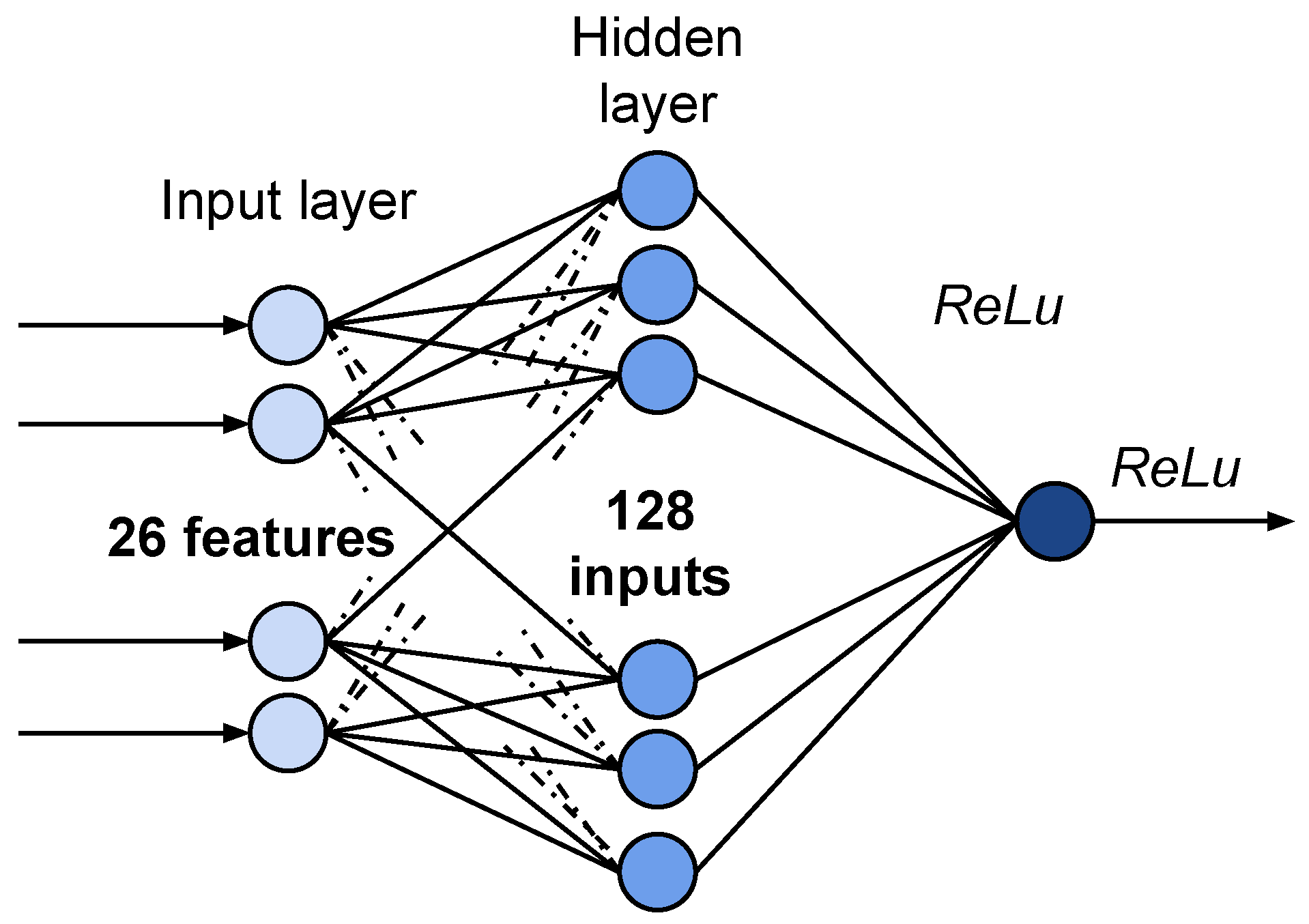
Figure 1 shows the architecture of a neural network for regression problems of predicting response time and loss probability. We used a brute force algorithm to select optimal neural network parameters by varying the number of hidden layers from one to two and the number of neurons from 64 up to 256. The network has one hidden layer with 128 perceptrons. We used Adam’s algorithm [28] to optimize the stochastic gradient descent. Activation function on the hidden and output layers was ReLu [29]. To train the ANN, the dataset was split into subsets (batches) of 512 copies. The number of epochs for training was equal to 1000.

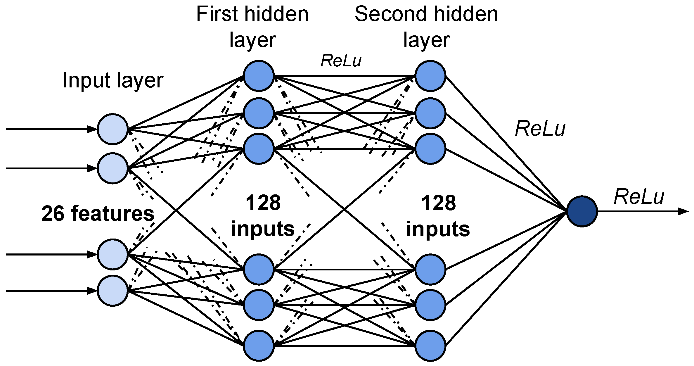
Figure 2 shows the neural network architecture for classification problems. We used brute force algorithm to select optimal neural network parameters. The network consists of an input layer with 26 inputs, two hidden layers with 128 perceptrons in each one, and an output layer. Each layer uses the ReLu activation function. As in ANN for regression problems, we used Adam’s algorithm to optimize gradient descent.

4.2.3. Generation of Synthetic Dataset for Machine Learning

The dataset is needed to train and test the ML model. We used the data obtained after repeated simulation model execution with different randomly generated input parameters to build this dataset. Let us discuss the synthetic input parameters generator in more detail.

All the numerical parameters are assumed to be uniformly distributed. For each of them we specify its minimum and maximum values.

To set the customers arrival rates ${\lambda }_k$, we explicitly select random arrival rates of the highest and lowest priority customers ${\lambda }_1,{\lambda }_K\in [{\lambda }_{min},{\lambda }_{max}]$, along with the approximation function $f_a$, ${\lambda }_k=f_a(k,{\lambda }_1,{\lambda }_K)$. This approximation function is randomly selected from the predefined set of functions. The same approach is used for customers service rates and the probabilities of customers joining the queue.

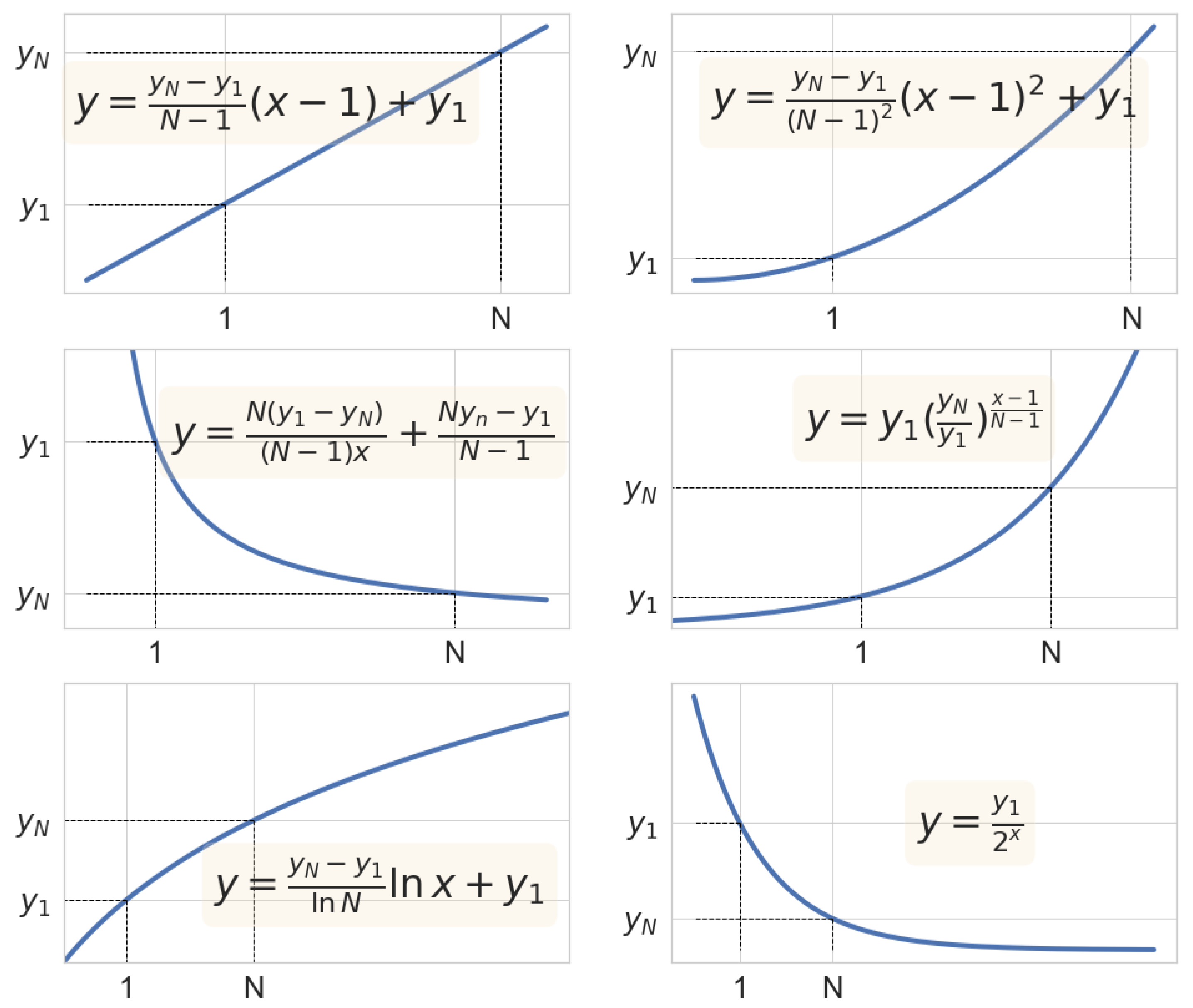
Figure 3 shows the set of approximation functions used for arrival rates ${\lambda }_k$ and service rates ${\mu }_k$ for customers types $k=\overline{1,K}$ calculation. This set includes:

• $F_c\left(n\right)\equiv C$, constant values;
• $F_l\left(n\right)=\frac{y_K-y_1}{K-1}(n-1)+y_1$, linear approximation;
• $F_p\left(n\right)=\frac{y_K-y_1}{{(K-1)}^2}{(n-1)}^2+y_1$, parabolic approximation;
• $F_h\left(n\right)=\frac{K(y_1-y_K)}{(K-1)n}+\frac{K{y}_K-y_1}{K-1}$, hyperbolic approximation;
• $F_e\left(n\right)=y_1{\left(\frac{y_K}{y_1}\right)}^{\frac{n-1}{K-1}}$, exponential approximation;
• $F_{log}\left(n\right)=\frac{y_K-y_1}{lnK}lnn+y_1$, logarithmic approximation;
• $F_g\left(n\right)=\frac{y_1}{2^n}$, geometric progression.

In all functions, n is an integer and takes values from $[1,2,\cdots ,K]$. To generate the probabilities of customers joining the queue, we used four functions:

• $H_1\left(n\right)\equiv 1$, customers always join the queue if it has space;
• $H_l\left(n\right)=-\frac{n-1}{K-1}+1$, linear approximation;
• $H_h\left(n\right)=\frac{1}{n}$, hyperbolic approximation;
• $H_g\left(n\right)=\frac{1}{2^{n-1}}$, geometric progression approximation.

Note that the accuracy of predictions obtained using ML methods depends on how representative is the training dataset. For example, suppose the system’s behavior on a particular set of input parameters differs significantly from everything observed in the training dataset. In that case, it will not be possible to obtain an accurate prediction at such an input. Because of this, we considered wide ranges for all input parameters, and the training sample was quite large (200,000 records). At the same time, it is crucial to avoid overfitting since the prediction accuracy also decreases.

The main limitation of our approach to describing input parameters is the use of the same coefficients of variation and skewness for service times and intervals between consumers of different types. It is easy to get around it, for example, using the same functional approach for setting the coefficients of variation and skewness that we used to set the arrival and service rates of intermediate types of customers. In this case, however, the input dimension will increase, and a larger dataset may need to be considered. In addition, more sophisticated and computationally expensive methods to $MMAP$ fitting will be needed.

5. Numerical Results

To study the performance of the priority queueing system using the proposed methodology, we conducted a series of numerical experiments:

• Firstly, we analyzed the analytic model complexity and used it to validate the simulation model based on Monte Carlo method.
• Secondly, we generated a synthetic dataset for training and testing ML models.
• Finally, we studied the accuracy of models predictions.

We compared customer loss probability, the average number of customers in the queue, and the average number of customers in the system during the simulation model validation. These metrics were computed for different values of queue capacity and servers number. All validations were passed, which showed that the simulation model is correct and can be safely used in the following experiments.

In the numerical experiments with ML models, we analyzed two characteristics of the priority systems: response time and loss probability of priority customers. In the scope of telecommunication networks, these characteristics are essential for verifying QoS compliance. However, our methodology allows studying any other characteristic, e.g., the average system size, number of high-priority customers, or number of busy servers. Furthermore, we investigated regression and classification problems using ML methods for both response time and loss probability.

The algorithm for computing stationary distribution of the system states that we described in Section 3 was implemented in Python language, as well as the simulation model interface. In addition, we used the C++ language to implement the core of the simulation model to improve performance. To connect Python interfaces and C++ core, we used Cython. Also, we used Jupyter Notebook to work with the dataset.

The source code of the project is available on GitLab: https://gitlab.com/lab69/priority-queues (accessed on 25 October 2021).

5.1. Complexity of the Analytical Model

Before moving on, we studied the bounds of size of the input, where results can be obtained with the analytical model. Since the number of customers in the analytical model is always equal to $K=2$, we varied the number of servers, the queue capacity, order of arrival $MMAP$, and $PH$ service times.

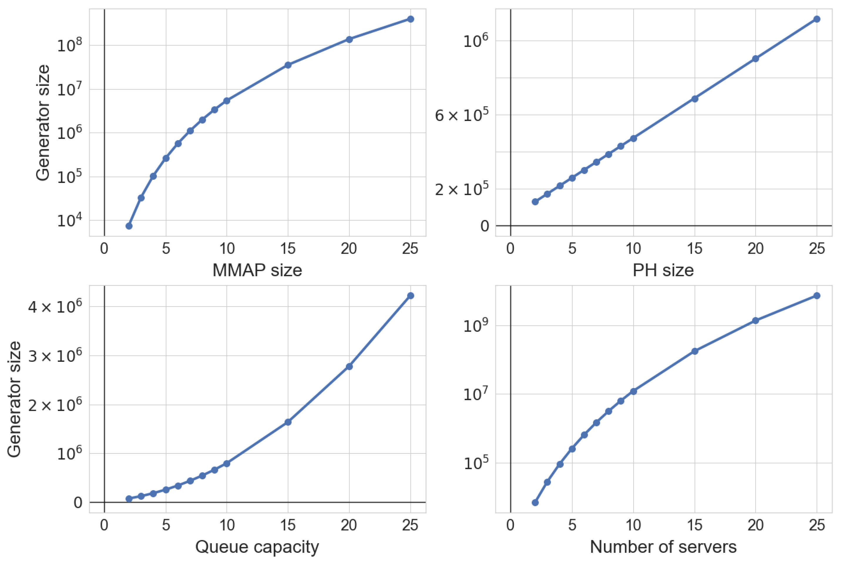
The key metric that defines the problem complexity is the order of the infinitesimal generator since it defines a linear equation system that needs to be solved to obtain the characteristic values. Figure 4 shows the dependency between the system generator order and the number of states in $MMAP$ or $PH$, queue capacity, and the number of servers. It can be seen that the generator complexity exponentially grows along with the order of $MMAP$ and the number of servers. However, it linearly depends on the order of $PH$ service time distributions and almost linearly on the queue capacity.

In general, for reasonably large input values, the generator is too big to be used to compute stationary states distribution and performance characteristics. For instance,

Table 1. Elapsed time to build the generator matrix.

No. of Servers	Time (s)
1	0.027
2	1.184
3	34.485
4	1155.581
5	Not enough RAM

provides measurements of time required to build the generator matrix depending on the number of servers. The experiment was conducted on a computer with an Intel Core-i7 processor and 16 GB of RAM. Although this particular limitation can be circumvented by using a more efficient matrix representation. The problem remains since the dependence of the generator order on the number of servers is exponential.

5.2. Validation of the Simulation Model

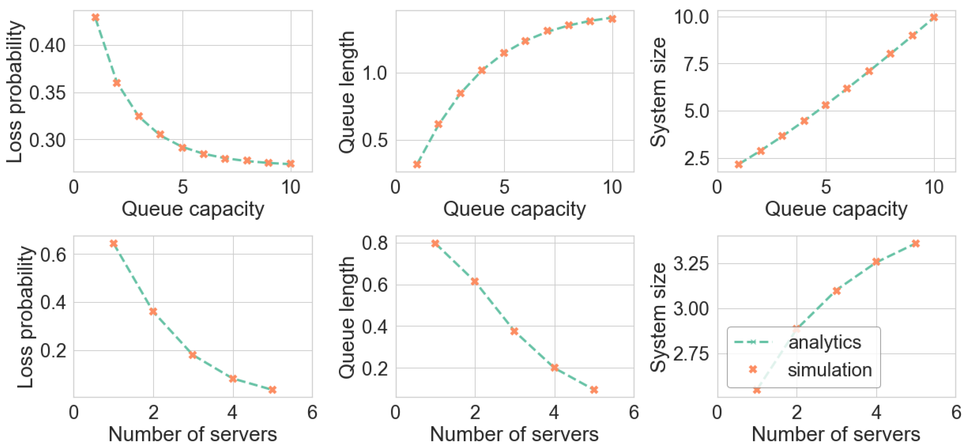
We used the analytical model to validate the simulation model implementation on reasonably small input values, where an analytical solution could be obtained. In these validations, we varied the number of servers and queue capacity and used different $MMAP$ flows and $PH$ service time distributions. For example, Figure 5 shows the results of comparing customer’s loss probability, queue size, and the number of customers in the system.

All validations were passed and showed that the simulation model provides numerical results with high precision. The relative error in the experiment does not exceed $0.5\%$. However, to reach high accuracy simulation model had to process about 1,000,000 customers for each input value, which required a reasonably large amount of time.

Simulation model validation was automated using the PyTest library. Each time the simulation model code changed, unit tests were executed to compare simulation and analytical results. This approach allows being sure that any change in the code does not break the model’s correctness.

5.3. Generation of the Dataset for Machine Learning Algorithms

To train and test ML models, we generated a large dataset with 200,000 random input vectors, as was described in Section 4. After that, the simulation model was used to get performance characteristics values for each input record in this dataset. Boundary values for all input parameters are shown in

Table 2. Boundary values for dataset generator.

Parameter	Min Value	Max Value
Number of customers types	1	5
Number of servers	1	10
Queue capacity	0	10
Arrival rate	0.1	10.0
CV of the arrival distribution	0.1	10.0
Skewness of the arrival distribution	-	100.0
Service rate	0.1	10.0
CV of the service time distribution	0.1	10.0
Skewness of the service time distribution	-	100.0

.

Note that the skewness did not have the minimum value. Instead, it was computed for the selected CV as described in [23].

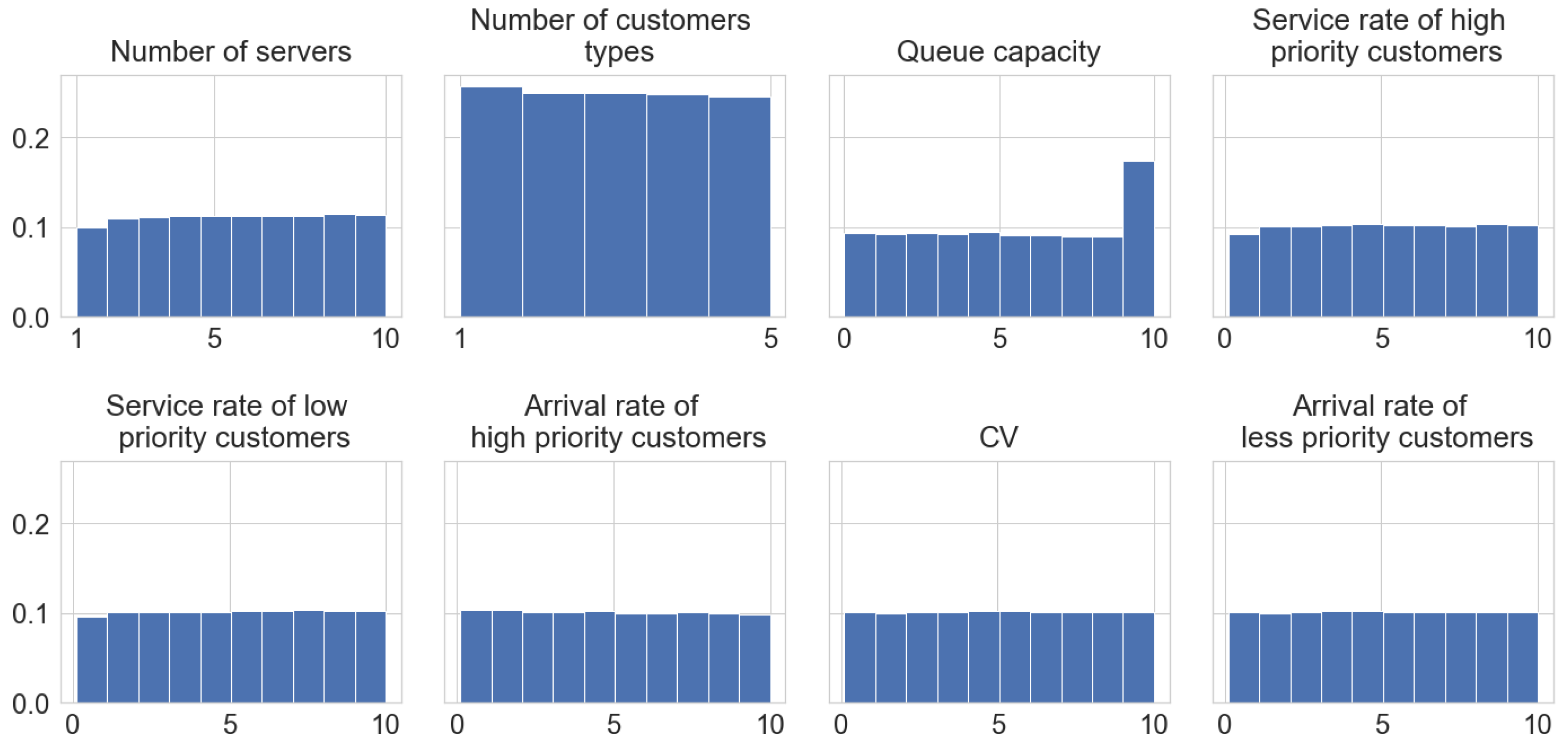
Figure 6 shows the histograms of different input parameters over the generated dataset. Most of the parameters are distributed almost uniformly; the only exception is the queue capacity. We forced the generator to include more samples with big capacity for the systems with a large number of customers types.

5.4. Prediction of System Response Time

The first performance metric we studied using machine learning methods was the system response time, i.e., the time the customer spends in the system from arrival to the end of the service. Regression models were used to predict the exact response time value. The classification models answered whether the system response time for the given input is less than a given threshold.

5.4.1. Regression Problem

We used decision trees, random forests, gradient boosting, and neural networks in the regression problem for predicting the system response time. To select the optimal hyperparameters for each algorithm, we used the grid search method. The optimal decision metric for the trees algorithms was chosen among MSE and MAE, and the max tree depth varied from 4 to 20. The number of predictors, a parameter specific for random forest and gradient boosting, was chosen from an array $[100,5000]$ with step 100. To estimate the accuracy of the algorithms, we used three metrics: the correlation coefficient, R2-coefficient, and the mean squared error.

Table 3. Hyperparameters for tree algorithms.

Algorithm	Metric	Max Depth	Number of Predictors
Decision tree	MSE	10	-
Random forest	MSE	16	500
Gradient boosting	MSE	12	1000

shows the optimal hyperparameters for tree algorithms. The optimal metric for each tree algorithm was the mean squared error. The maximum tree depth was equal to 16 for the random forest algorithm.

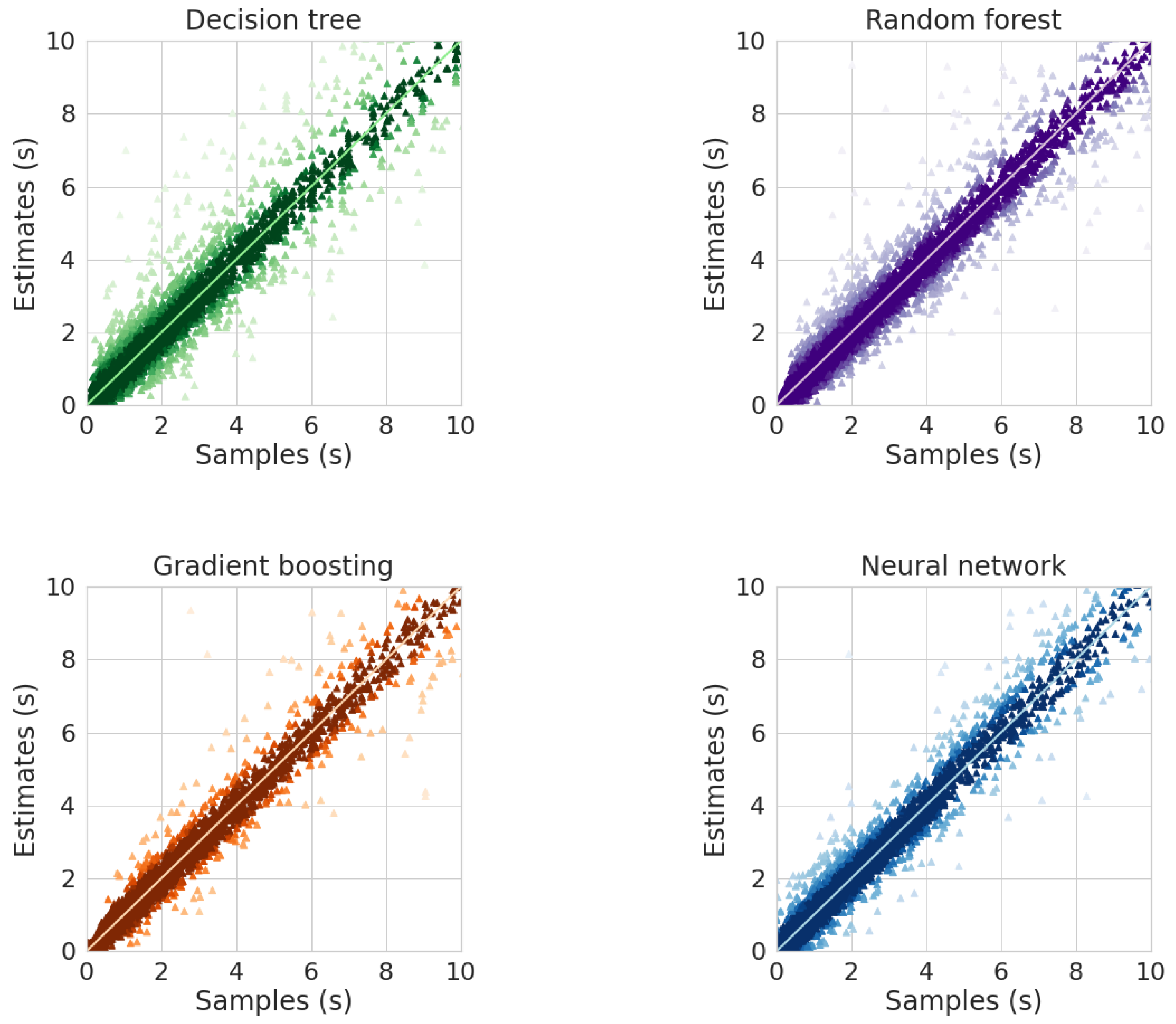
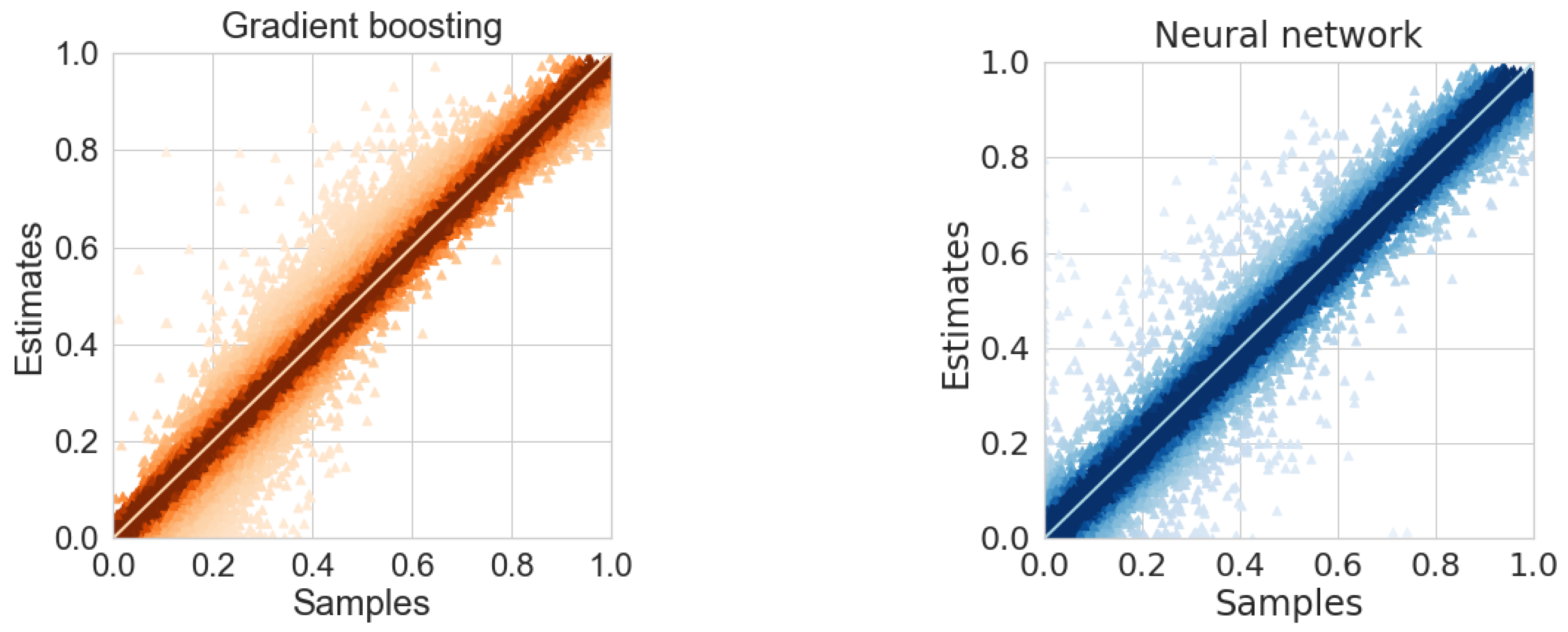
Figure 7 shows the scatter diagrams for ML algorithms. The decision tree algorithm demonstrates the largest scatter and error; in some cases, the relative error reaches $20\%$.

Table 4. Metric values for regression models for system response time.

Algorithm	Correlation	R2	MSE
Decision tree	0.944	0.891	0.135
Random forest	0.980	0.961	0.047
Gradient boosting	0.980	0.961	0.047
Neural network	0.987	0.973	0.031

shows the metric values for regression models for system response time prediciton. The random forest algorithm and gradient boosting demonstrate similar results for all metrics. The best results for all metrics were obtained with the neural networks.

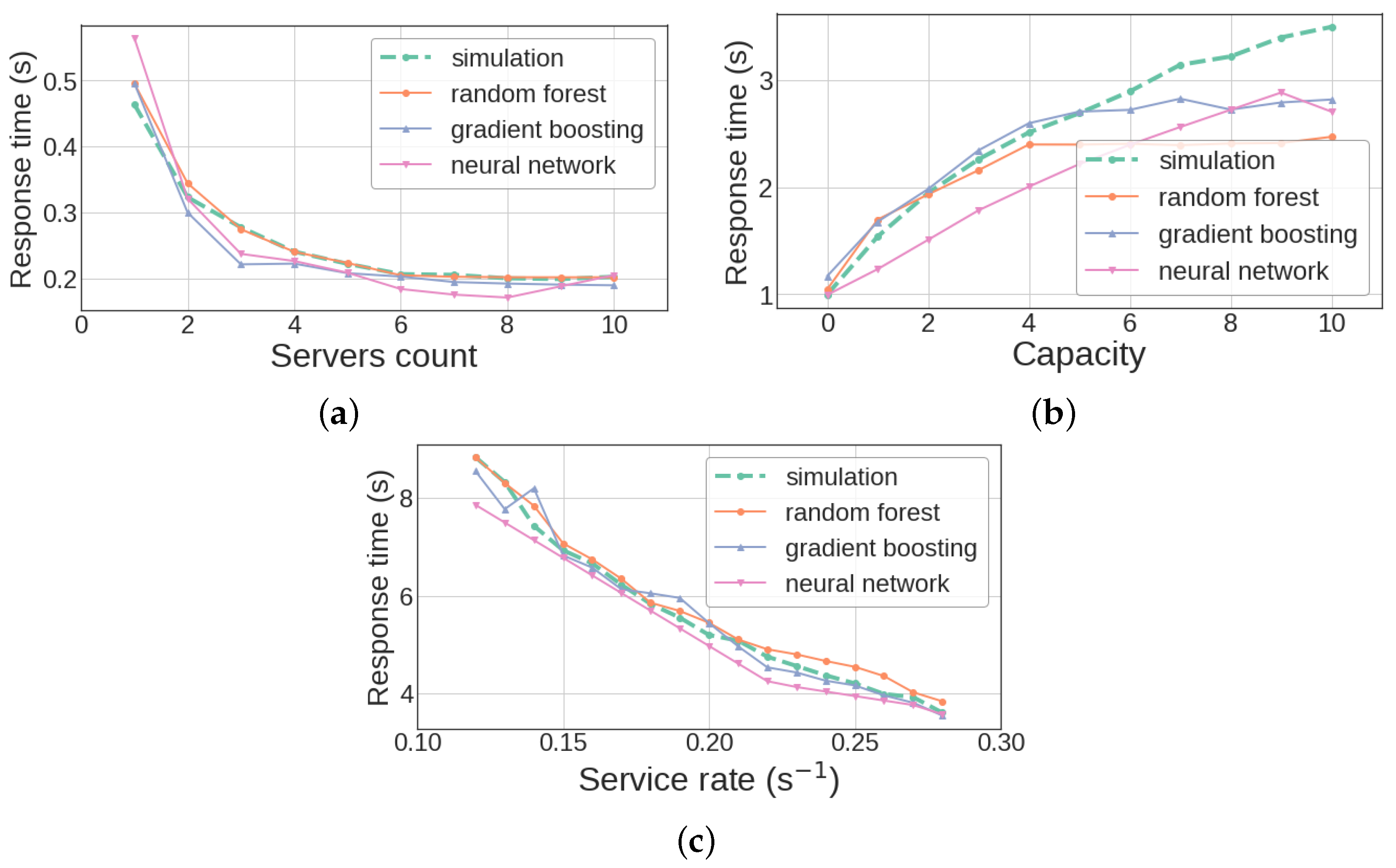
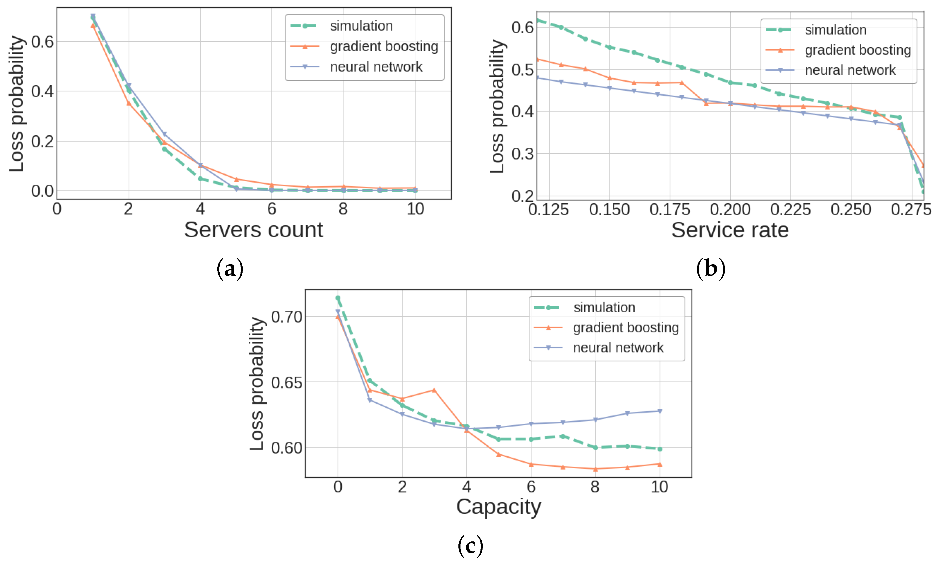
We analyzed the dependency between the system response time and the number of servers, service rate of high priority customers, and queue capacity to validate the models. In each case, the system response time was computed using the simulation model and each trained ML model.

In the first experiment, the number of servers varied from 1 to 10, while other parameters were fixed: $K=3$, $c_a=5$, ${\gamma }_a=50$, $f_a=F_l$ (linear approximation of arrival rates), ${\lambda }_1=4.0$, ${\lambda }_K=5.0$, $c_s=5$, ${\gamma }_s=50$, $g_s=F_l$, ${\mu }_1=4.0$, ${\mu }_K=5.0$, $R=10$, $h=1$. Figure 8a shows the results. In this case, the random forest algorithm demonstrates the most accurate results, while the neural network prediction is the worst. The maximum error in random forest prediction arises for the system with a single server.

In the second experiment (see Figure 8b)) we varied the queue capacity from 0 up to 10 and set other parameters to $K=2$, $c_a=5$, ${\gamma }_a=50$, $f_a=F_l$, ${\lambda }_1=2.0$, ${\lambda }_K=1.0$, $c_s=5$, ${\gamma }_s=50$, $g_s=F_l$, ${\mu }_1=1.0$, ${\mu }_K=5.0$, $N=1$, $h=1$. In contrast to the previous experiment, the neural network gives here the highest accuracy, while the random forest has the greatest error.

In the third experiment (see Figure 8c) the service rate of the highest priority customers was varied from $0.01$ to $0.3$, while the other parameters were fixed: $K=3$, $N=5$, $c_a=5$, ${\gamma }_a=50$, $f_a=F_l$, ${\lambda }_1=1.0$, ${\lambda }_K=1.0$, $c_s=5$, ${\gamma }_s=50$, $g_s=F_l$, ${\mu }_1=0.1$ ${\mu }_K=1.0$, $R=1$, $h=1$. Random forest and gradient boosting has the highest accuracy, while the neural network gives the worst prediction, especially when the service rate is small.

5.4.2. Classification Problem

In many practical applications, the exact value of the system response time is not important. Instead, we may be interested in whether the response time is short enough. To answer this question, we trained several ML models to classify the priority queueing systems depending on the expected value of the response time. As a threshold, we assumed the response time equal one second, i.e., the system belongs to the first class if its response time is more than one second; otherwise, it belongs to the second class.

In addition to decision trees, random forests, gradient boosting and neural networks, we used logistic regression [30] as this is the simplest ML method applied to classification problems.

Table 5. Comparison of various machine learning methods for the response time classification problem.

Algorithm	Precision	Recall	F1 Score
Logistic regression	0.93	0.90	0.92
Decision tree	0.94	0.95	0.95
Random forest	0.98	0.92	0.95
Gradient boosting	0.98	0.96	0.97
Neural network	0.96	0.96	0.96

shows the results of the accuracy comparison.

The experiment result shows that gradient boosting and neural networks provide the most precise results. As expected, the logistic regression algorithm is less effective than any other algorithm being used [31,32].

5.5. Prediction of the Priority Customers Loss

The second metric we studied using ML methods was the probability of losing the customer with the highest priority. According to the assumptions in Section 4.2.1, the highest priority customer may be lost in the only case that the queue is full. As in the response time prediction, both regression and classification problems were considered.

5.5.1. Regression Problem

To solve the regression problem for predicting the loss probability, we used only two algorithms: a gradient boosting and neural network. Early experiments showed that the decision tree and random forest give an unacceptably high error. Therefore, we trained two models and compared the results.

Gradient boosting algorithm and neural network show similar results (see

Table 6. Metrics values for ML algorithms of high priority customers loss probability.

Algorithm	Correlation	R2	MSE
Gradient boosting	0.982	0.964	0.003
Neural network	0.984	0.966	0.003

); their metrics are practically the same. Figure 9 demonstrates that the neural network has the same absolute error for all samples. As for gradient boosting, it provides a larger absolute error when samples values (that is loss probability) are close to zero.

To validate ML models for loss probability prediction we used the similar validation datasets as for response time validation. Figure 10a–c show the numerical results.

5.5.2. Classification Problem

The classification models define whether the probability of losing a priority customer is greater than $0.1$. We used logistic regression, tree algorithms, and neural network algorithms for classification problems. Results in

Table 7. Comparison of ML algorithms for classiification priority systems by loss probability value.

Algorithm	Precision	Recall	F1 Score
Logistic regression	0.86	0.85	0.86
Decision tree	0.87	0.89	0.88
Random forest	0.93	0.94	0.93
Gradient boosting	0.95	0.95	0.95
Neural network	0.97	0.98	0.97

shows that the neural network provides the best precision.

5.6. Analysis of Elapsed Time

To use machine learning algorithms, they need to be trained, which takes a significant amount of time. For example,

Table 8. Learning time for regression ML models.

Model	Time (s)
Decision tree	$5\times {10}^{-5}$
Random forest	556
Gradient boosting	1086
Neural network	1201

shows the time it took to train on a dataset with 200,000 records of decision tree algorithms, random forests, gradient boosting, and artificial neural networks.

Neural network training takes about 1200 s for 1000 epochs. The batch size equals 8192, the average time for epoch is about 1 s.

Table 9. Time elapsed for prediction of response time.

Algorithm	Time (s)
Analytics	35
Simulation model	2
Decision tree	$2\times {10}^{-7}$
Random forest	$6.8\times {10}^{-5}$
Gradient boosting	$1.6\times {10}^{-5}$
Neural network	$2.1\times {10}^{-6}$

shows the typical time that is required for estimation of system response time by analytical model, Monte Carlo method, and trained ML algorithms. For $MMAP$ and $PH$ distributions of reasonably small size, it took about 35 s to compute response time using the analytic method. In the same case, the Monte-Carlo method is ten times more efficient than the analytics algorithm. It is worth noting that the complexity of the analytical model grows exponentially, so in general, the simulation model is the only way to estimate the performance characteristics of the systems of arbitrary size.

At the same time, the performance of ML algorithms is more than ${10}^5$ times better than the simulation model. Thus, while we needed to spend a significant amount of time generating a synthetic dataset and training machine learning algorithms, this time is fully compensated by the gain from the trained algorithms if estimates need to be obtained a very large number of distinct input vectors.

6. Conclusions

In this paper, we investigated the multi-server priority queueing system with correlated arrival $MMAP$ flow of arbitrary number K of types of customers and finite queue. The type of the customer defines its priority, service time distribution, and the probability that the customer will join the queue when all servers are busy. Such systems are practically not studied in the literature. We presented an analytical solution for the system with two types of customers, calculated stationary distribution of the system states, and main performance measures, including average system size, the average number of priority customers, customer loss probability, and the number of busy servers.

The analytical model has a very high computational complexity, exponentially dependent on the number of servers and order of $MMAP$. Thus, in the numerical experiment, we could compute the model characteristics for systems with only four servers, while adding one more server led to memory overrun. Another limitation of the analytical model is that it supports only two classes of customers. To overcome these limitations, we described a new methodology for the fast estimation of system characteristics using a combination of simulation modeling (based on the Monte Carlo method) and machine learning. We conducted numerical experiments, showing that the proposed methodology allows estimating characteristics with high precision, up to 96–98%. Furthermore, estimation on the given input with a trained ML model requires several orders of magnitude less time than the barebone Monte Carlo method. As for machine learning methods, random forest and gradient boosting showed similar results in regression and classification problems for priority packets response time and loss probabilities.

The proposed methodology provides means for using the priority queueing system model in complex optimization problems, appearing in the design and implementation of modern telecommunication networks, where the traffic is essentially heterogeneous.

We plan to improve the algorithm’s performance for queueing system characteristics computation by using more advanced numerical techniques and sparse matrices. This idea is based on the observation that the generators are block matrices with lots of zeros. While this improvement can not solve the problem of exponential growth of the state space, it may help expand the area where the precise solution may be found. We also plan to explore the possibilities of using machine learning methods to solve other problems of queuing theory that cannot be solved using traditional methods. Finally, we are also working on the development of methods for applying the proposed model to estimate the characteristics of real technical telecommunication systems. The results of these researches will be presented in future papers.