Application of Machine Learning Model for the Prediction of Settling Velocity of Fine Sediments

Abstract

Sedimentation management is one of the primary factors in achieving sustainable development of water resources. However, due to difficulties in conducting in-situ tests, and the complex nature of fine sediments, it remains a challenging task when dealing with issues related to settling velocity. Hence, the machine learning model appears as a suitable tool to predict the settling velocity of fine sediments in water bodies. In this study, three different machine learning-based models, namely, the radial basis function neural network (RBFNN), back propagation neural network (BPNN), and self-organizing feature map (SOFM), were developed with four hydraulic parameters, including the inlet depth, particle size, and the relative x and y particle positions. The five distinct statistical measures, consisting of the root mean square error (RMSE), Nash–Sutcliffe efficiency (NSE), mean absolute error (MAE), mean value accounted for (MVAF), and total variance explained (TVE), were used to assess the performance of the models. The SOFM with the 25 × 25 Kohonen map had shown superior results with RMSE of 0.001307, NSE of 0.7170, MAE of 0.000647, MVAF of 101.25%, and TVE of 71.71%.

1. Introduction

1.1. Background and Problem Statement

The movement characteristics of sediments (i.e., coarse and fine sediments) are considered as one of the most complex study areas in the field of hydrology. Shallow riverbeds were one of the main causes of flood-related disasters reported worldwide, with an estimated financial loss of almost USD1800/s between 1990 and 2020 [1]. Sedimentation issues have always been a deep concern for various parties due to the severe impacts that are invited by sediments. Siltation, for instance, is a critical problem that is caused by the resuspension of fine sediments deposited within the sediment bed in water [2,3]. Siltation could also induce a large number of negative impacts on humans and the environment. For example, changes in water flow patterns and bed structure, a reduced lifetime of reservoirs, aggravation of floods, deterioration of water quality leading to a shortage in water supply, and destruction of natural habitats which threatens the aquatic biodiversity [4,5]. Economically, stakeholders would need to bear exorbitant costs on their projects, such as carrying out landfilling and water treatment activities. Fine sediments are the root causes of the siltation possess [6,7]. The transport mechanism of fine sediments is known to take place in locations ranging from rivers, reservoirs, dams, lakes, to coastal areas, for which the flow structures, bed morphology, as well as water quality are highly affected [8,9].

Understanding the seriousness and series of negative impacts from sedimentation problems, many studies related to sedimentation have been conducted in the past few decades. The transport mechanism of sediments could be fundamentally described by two main processes: the horizontal advection, and the vertical sedimentation that is due to gravitational acceleration [10,11]. In the past, there were several commonly used sediment-related parameters, such as water turbidity [12], salinity [13], suspended sediment concentrations [14], and total suspended solids [15]. Although some of the basic indications of the sediment loadings in the water could be presented, such parameters were inadequate in describing the hydrodynamics of fine sediment since the vertical flux, which is the essential component of sedimentation, was not considered [16,17].

Furthermore, the increase in complexity of fine sediment transport in water bodies was also driven by various factors which influence the relationship between water flow and fine sediment transport, including concentration, size, and surface electrostatic charge distributions of particles, bed structures, and flow rates. However, it is practically not feasible to determine precise measurements of these parameters on both temporal and spatial scales, where in-situ experiments and tests are required to be conducted [14,18].

The settling velocity, also known as terminal velocity, plays an important role in terms of interpreting hydrodynamic behaviors exhibited by fine sediments in water [9,19]. Specifically, the settling velocity is the velocity attained by fine sediments resulting from the balanced force between drag forces, gravitational pull, and other hydrodynamic forces [20]. For turbulent flows in particular, drag coefficients vary in accordance with the hydrodynamic forces, such as shear lift, buoyancy, Magnus force, and torque [21]. In this regard, the settling velocity accounts for the vertical flux in the process of sedimentation for different conditions. Thus, it is capable of providing a significant characterization of the hydrodynamics of fine sediments [22].

1.2. Machine Learning Model

There are numerous machine learning algorithms that perform classification and prediction tasks with different purposes, such as decision trees, random forests, long short-term memory networks, etc. [23,24] Being one of the pioneers of the machine learning models, an artificial neural network (ANN), which also operates machine learning algorithms, has been broadly employed in different contexts. This includes the field of green energy [25], business/economics [26], and health care [27]. In hydrology, countless studies have also taken advantage of ANN models, such as water quality predictions [28], wastewater treatment [29], flow duration curves modelling [30], turbulent flow velocity field prediction [31], adsorption water desalination system modelling [32], suspended sediment and sediment yield [14,24,33], ocean bubbles [34], and wall slip [35,36].

Essentially, ANN is technologically advanced as a generalization of mathematical models inspired by human cognition which depends on the biological neural system [13]. ANN, also often being referred to as black-box models, possesses flexibility in terms of mathematical computations and topography, making them capable of performing predictions, classifications, and modelling different types of complex and non-linear relationships between data inputs and outputs without prior interpretation of the data behavior [37]. Subsequently, diverse network architectures allowed ANN models which are conceptually semi-parametric regression estimators to be favored over other typical models. The basic development of ANN is generally based on, but not limited to, the given rules, i.e., (i) input information processed individually at multiple elements called neurons, also referred to as units, cells, or nodes; (ii) processed signals transferred between the neurons through the connective links; (iii) each of the connective links carries an associated weight, representing its connection strength; (iv) each neuron which typically applies a non-linear transformation to its net input to determine its output.

A typical ANN (see Figure 1) usually comprises three components, namely the input layer, hidden layer, and output layer. The input layer commences the algorithm, where it inputs one instance of the data into the network. The dimension of the instances determines the number of inputs in the input layer. The hidden layer contains one or several layers where it outputs intermediate data to the output layer, generating the final output of the network. The output number is determined by the encoding of the classified or estimated results. Each layer of the ANN consists of a specified number of neurons which determines the ANN network architecture.

Apart from the network architecture, there are two kinds of network parameters, weight, W, and bias, B, playing an important part in the learning and predicting process. Essentially, the concept of computational procedure involving both network parameters mimics the biological afferent and efferent neurons in transmitting signals [13]. At first, the afferent response is initiated when all the input signals are channelled into a particular neuron. As described in Equation (1), the net input value will be computed based on the total weights contributed by each input observation, x, added with a constant bias. The efferent response takes place once the net input is obtained. Based on the pre-defined activation function within each neuron, a single value output will be computed. There are different types of activation functions, but the most commonly implemented ones are the linear activation function, sigmoid/logistic activation function, and hyperbolic tangent activation function [38].

$$\mathrm{Net} \mathrm{Input}=\sum \mathit{W}\mathit{x}+\mathit{B}$$

(1)

It should be noted that in the training phase, a basic ANN employs feed-forward to generate an output, and then calculates the error between the output and the target output. In the prediction phase, a basic ANN will only execute a feed-forward mechanism to achieve the ultimate result. The approach of trial and error was implemented since there was no generally proven theory or fixed rule on the decision of the network geometry (i.e., the number of neurons and hidden layers) that ensures optimum prediction and classification results [39,40].

1.3. Research Objective

Regarding the ability in handling tedious computational tasks, machine learning-based models present an innovative alternative for the prediction of settling velocity of fine sediments. The main objective of this study is to propose machine learning-based computational models for the prediction of settling velocity of fine sediments. Three machine learning-based models were employed, along with four hydraulic as input variables to estimate a single output of the settling velocity of fine sediments. The relationship between the settling velocity and the input variables was then investigated. In addition, a comparative statistical analysis was carried out on the developed models based on their performance.

2. Methodology

The design of experimental procedures and data collection via advanced laboratory equipment, known as particle image velocimetry (PIV), was based on the main source of reference in the work of Kashani et al. [18]. In general, the whole-flow-field technique of the PIV records the position-over-time of the injected small tracer particles (seeds) in the flow [41], providing instantaneous velocity fields and real-time movements of fine sediments in the water.

This study emphasized the prediction of settling velocity of fine sediments by applying three distinct machine learning-based models, namely the radial basis function neural network (RBFNN), the backpropagation neural network (BPNN), and the self-organizing feature map (SOFM). The prediction models were developed based on the four hydraulic parameters as input variables, which consist of particle size (5 µm, 10 µm, 20 µm, 50 µm), inlet depth (6 cm, 7 cm, 8 cm, 9 cm, 10 cm, 10.5 cm), the relative x-position ranged between 0 cm and 50 cm, and the relative y-position ranged between 0 cm and 20 cm in the water column. The overall research methodology is shown in Figure 2.

To ensure machine learning-based models are well-trained, and, at the same time, achieve high performance with good generalization, the data set must be at least divided into two sets, namely the training set and testing set. However, different proportion settings on the division of training and testing data set were discovered in different studies, as no fixed proportion could guarantee the best results. Nonetheless, a typical range of 60% to 80% on the training set associated with 40% to 20% of the testing set were implemented [42,43,44]. As an initial attempt to estimate the settling velocity of fine sediments in this study, a stipulated proportion of 80%:20% (training set:testing set) was defined such that sufficient learning instances were allocated for the model training while reserving reasonable data size for model testing.

For the data pre-processing step, the min-max normalization technique was applied to the data before the training process was executed. The primary reason for the data normalization was to geometrically nullify the weight effects imposed by the input variables of incompatible scale units, range and interval values, and distributions into a desired compact and specific range [45]. In other words, normalization simplifies interpretation tasks in terms of the total variation contributed by the input variables, for which imbalanced weights over-influencing the learning of instances were minimized [46].

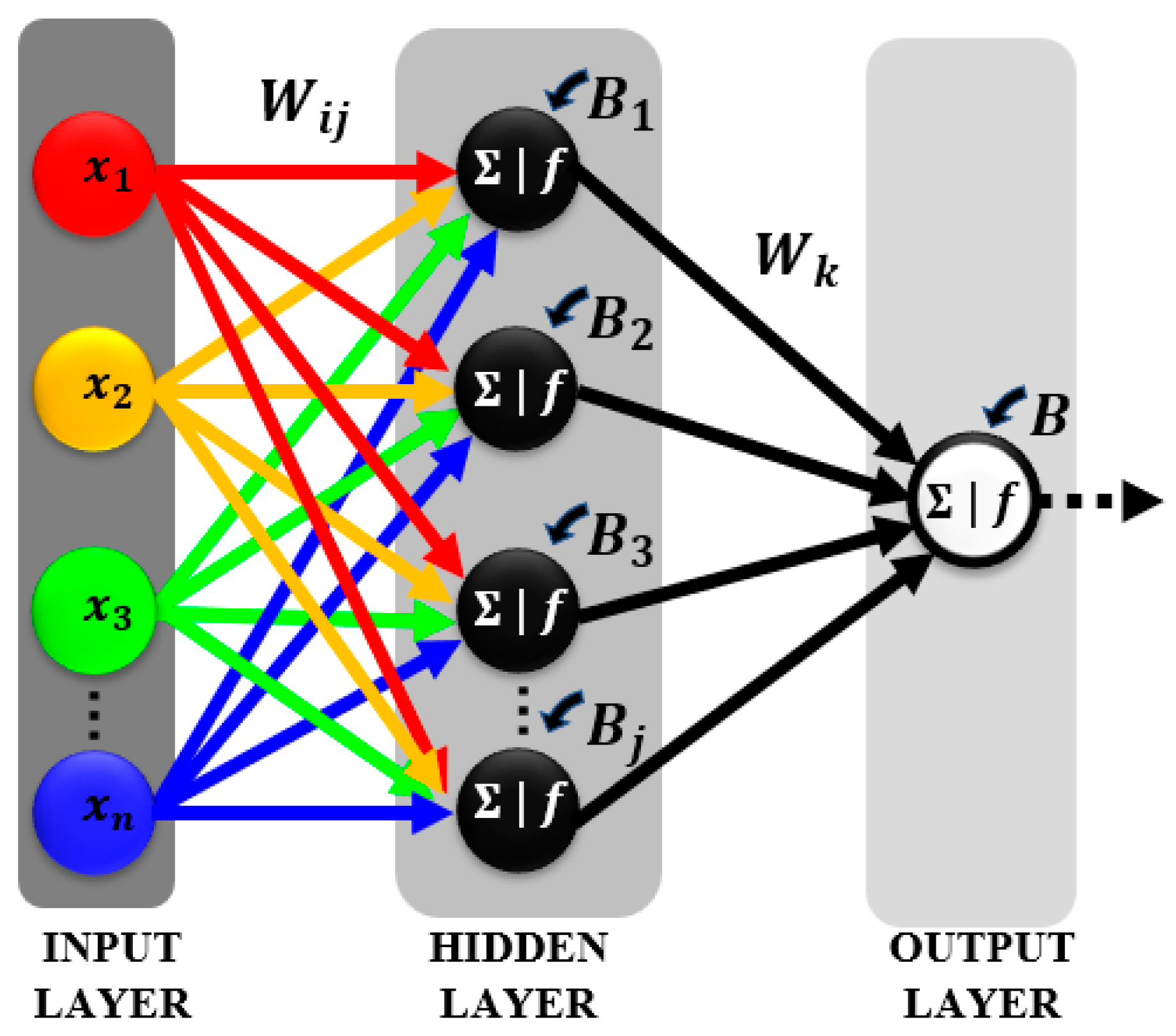
2.1. Radial Basis Function Neural Network (RBFNN)

The RBFNN takes a simple and straightforward form, and has been notably employed in different works, such as predicting suspended sediment load, and water turbidity in rivers [38,47]. RBFNN often requires a shorter time to be trained because of its simplistic structure of only three layers, namely the input layer, hidden layer, and output layer. The incoming input variables from the input layer of the RBFNN were fed forwarded to its hidden layer. The corresponding weights received by neurons in the hidden layer process these weights by computing them using the activation function. The specialty of RBFNN lies in the application of radial basis activation function (i.e., Gaussian) [48], as defined in Equation (2).

$$f\left(z\right)=\exp \left(\frac{{\parallel z-\mu \parallel }^2}{2{\sigma }^2}\right)$$

(2)

The parameters $\mu$ and ${\sigma }^2$ represent the mean and variance of the received weights specifying the central tendency and spread of the Gaussian curve [15,23]. The monotonic property held by the radial basis activation function with a good local convergence rate is the merit of the RBFNN. The network architecture of the proposed RBFNN was illustrated in Figure 3.

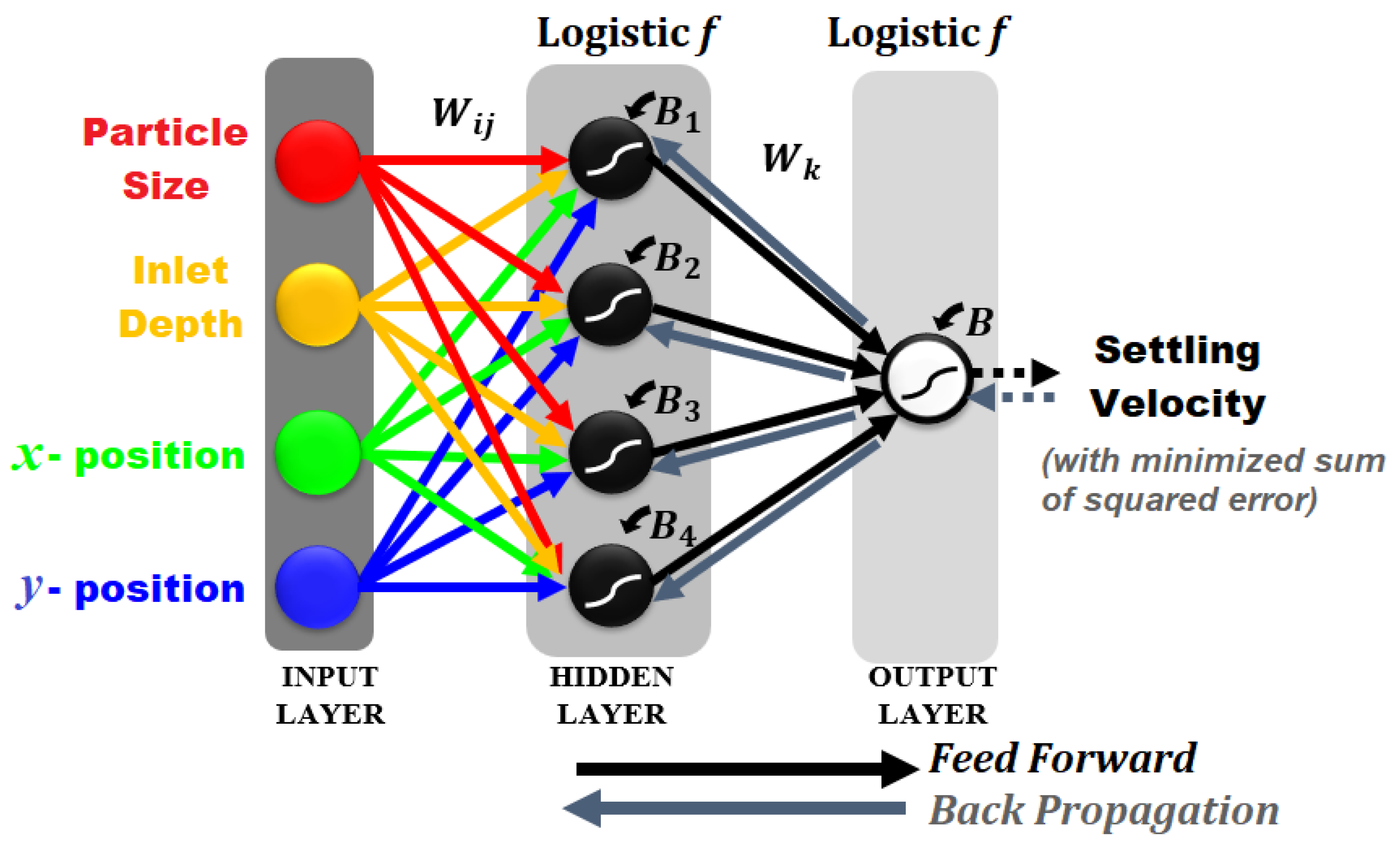
2.2. Back Propagation Neural Network (BPNN)

The BPNN is a well-known network that has been extensively applied in hydrology to predict and solve various problems, especially in water resources and management [49]. It shares the same network geometry as a basic ANN by having an input layer, an output layer, and one or more hidden layers. Fundamentals of the backpropagation algorithm in the case of control theory were discovered in the work of Kelley [50]. After training the BPNN with the input instances, the backpropagation learning algorithm allows the weights and biases parameters within the neurons to be tuned according to the Levenberg–Marquardt approach. In the tuning process, the network parameters are updated based on the minimization of the error functions [51,52]. In this study, the logistic activation function, as defined in Equation (3), was adapted, and the sum of squared error between the estimated and observed settling velocity is minimized. The network architecture of the proposed BPNN was illustrated in Figure 4.

$$f\left(z\right)=\frac{1}{1+\exp \left(-z\right)}$$

(3)

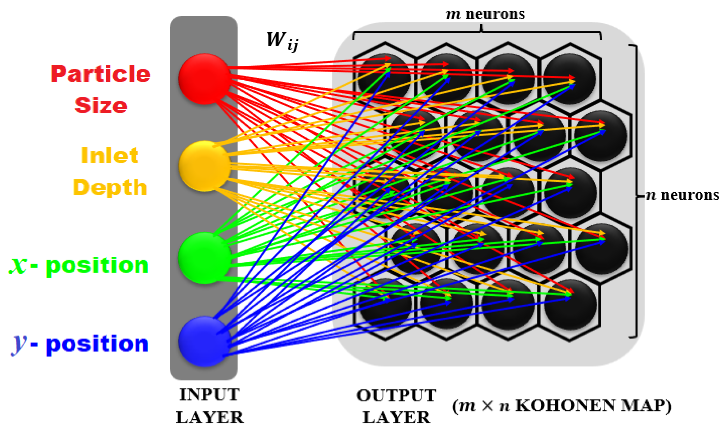
2.3. Self-Organizing Feature Map (SOFM)

The SOFM, with its unique network architecture, was initially proposed by Kohonen [53,54]. With the growing interest in the application of unsupervised learning algorithms, SOFM has been widely used, mostly for data classification and estimation. Studies that implement SOFM, relevant to the field of hydrology, include the characterization and survey of groundwater chemistry and groundwater levels [55,56], sediment quality assessment [4], and soil hydraulic properties [57]. However, there were hardly any recent applications of the SOFM related to fine sediment studies, specifically in estimating hydrodynamic characteristics of fine sediments. The SOFM consists of only an input and a Kohonen map. The Kohonen map is a discrete lattice structure of usually two dimensions, formed by the projection of multidimensional inputs through a non-linear vector quantization-based learning attribute. Neurons in the Kohonen map are physically arranged in a hexagonal fashion while the topological properties of the input space are preserved. The network architecture of the proposed SOFM is illustrated in Figure 5.

For each iteration step, $s$, the Euclidian distance was computed between the input vector, $z$, and the neurons in the Kohonen map. Out of the $M$ neurons in total, the best matching unit (BMU), $\theta$, served as the winning neuron after competing with other neurons. Thus, the BMU possesses the minimum Euclidian distance towards the input vector, as shown in Equation (4).

$${D_j}^{\left(\theta \right)}=\underset{1\le j\le M}{\mathrm{argmin}}\parallel z_i\left(s\right)-w_{ij}\left(s\right)\parallel$$

(4)

Once the BMU is selected, the weight vectors of the neurons located within the pre-defined neighborhood function (Gaussian) shown in Equation (5) were then updated cooperatively. The Euclidean distance between a neuron and the BMU acts as the central mean of the Gaussian neighborhood, whereas the learning rate, $\delta$, as defined in Equation (6), determines the corresponding spreadness. Both the learning rate, and neighborhood radius, $\eta$, as defined in Equation (7), decreased accordingly when iterations were increased. Consequently, Equation (8) shows the updating rule for the weights in each neuron within the neighborhood of BMU.

$$H_{\theta }\left(s\right)=\exp \left(-\frac{{\parallel \theta -{\theta }^{*}\parallel }^2}{2{\left(\delta \left(s\right)\right)}^2}\right)$$

(5)

$$\delta \left(s\right)=\delta \left(0\right)\exp \left(-\frac{s}{T}\right)$$

(6)

$$\eta \left(s\right)=\frac{\eta \left(0\right)}{s}$$

(7)

$$w_{ij}\left(s+1\right)=w_{ij}\left(s\right)+\delta \left(s\right)\left[z_i\left(s\right)-w_{ij}\left(s\right)\right]$$

(8)

Eventually, clusters of similar neurons can be identified as the training process matures. Individual heat maps could be produced for visualization purposes to enhance the study of the relationship between the input parameters with the settling velocity. As the neighborhood function provides close density estimation in the Kohonen map, the prediction of settling velocities was based on the asymptotic convergence to the mean value computed from the values within the BMU, $\overline{V}{ }^{\left(\theta \right)}$, as defined in Equation (9).

$$\widehat{V}=\overline{V}{ }^{\left(\theta \right)}$$

(9)

2.4. Performance Measures

For $N$ of the settling velocity observations, $V_k$, and their corresponding predicted values, ${\widehat{V}}_k$, the average value is represented by $\overline{V}$. The following Equations (10)–(14) show the five types of statistical measures applied to access the prediction performance of the developed machine learning models.

(i)

Root mean square error (RMSE):

$$RMSE=\sqrt{\frac{{{\displaystyle \sum }}_{k=1}^N{\left({\widehat{V}}_k-V_k\right)}^2}{N}}$$

(10)

(ii)

Nash–Sutcliffe efficiency (NSE):

$$NSE=1-\frac{{{\displaystyle \sum }}_{k=1}^N {\left(V_k-{\widehat{V}}_k\right)}^2}{{{\displaystyle \sum }}_{k=1}^N {\left(V_k-\overline{V}\right)}^2}$$

(11)

(iii)

Mean absolute error (MAE):

$$MAE=\frac{{{\displaystyle \sum }}_{k=1}^{N } \left|V_k-{\widehat{V}}_k\right|}{N}$$

(12)

(iv)

Mean value accounted for (MVAF):

$$MVAF=\left[1-\frac{{{\displaystyle \sum }}_{k=1}^N \left(V_k-{\widehat{V}}_k\right)}{{{\displaystyle \sum }}_{k=1}^N{V}_k}\right]\times 100\%$$

(13)

(v)

Total variance explained (TVE):

$$TVE=\left[1-\frac{var\left(V_k-{\widehat{V}}_k\right)}{var\left(V_k\right)}\right]\times 100\%$$

(14)

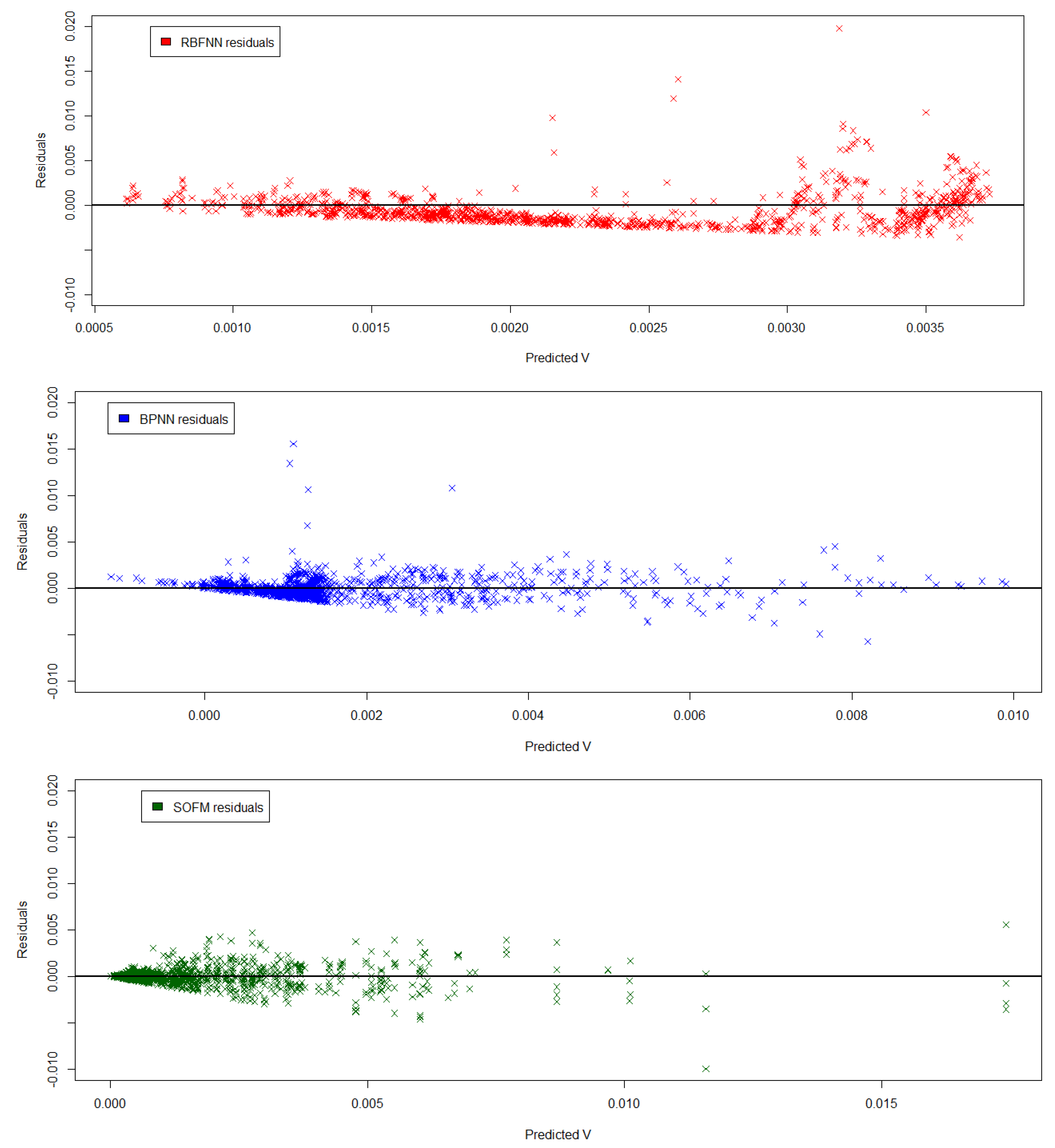
3. Results and Discussion

Under the method of trial and error, the optimum network parameters and geometry were decided based on the performance measures computer for each of the models. To compare and contrast the three developed machine learning-based models, the most appropriate model with the highest accuracy was determined once the best parameter settings were finalized. Ideally, the RMSE and MAE should be close to zero, indicating the minimum error obtained; the NSE should be close to 1, indicating the model is better than applying the mean estimator; the MVAF should be close to 100%, indicating the accuracy of the average estimating performance of the model; the TVE should be close to 100%, indicating the overall dynamics and dispersion accounted by the model.

Due to the flexible settings of network architectures, numerous combinations of network parameters and geometry could be generated. Consequently, only selected models that provided appropriate results relevant to the performance measures were reported.

Table 1. Results of the RBFNN model with different network architectures.

Network Architecture *	RMSE	NSE	MAE	MVAF (%)	TVE (%)
4-10-1	0.002739	0.1409	0.001616	195.21	20.37
4-11-1	0.002666	0.1469	0.001493	187.87	20.27
4-12-1	0.002798	0.1333	0.024785	200.47	19.94
4-13-1	0.002681	0.1442	0.001898	189.09	20.05
4-14-1	0.002800	0.1261	0.001477	199.34	18.73
4-15-1	0.002717	0.1400	0.001527	192.50	19.89
4-16-1	0.002667	0.1478	0.001409	188.18	20.43
4-17-1	0.002495	0.0966	0.001504	153.50	11.02
4-18-1	0.002711	0.1435	0.002134	192.51	20.38
4-19-1	0.002760	0.1370	0.001420	196.88	20.03
4-20-1	0.002502	0.1196	0.001483	160.03	14.08

* The RBFNN network architecture is defined based on the sequence of ‘input neurons-hidden neurons-output neuron’.

shows the results of the RBFNN model. The lowest RMSE of 0.002495 and MAE of 0.001409 were seen at the 4-17-1 setting, but the optimum values of NSE, MVAF, and TVE were 0.1435%, 188.18%, and 20.43%, respectively, which was exhibited by the 4-16-1 setting. Thus, the 4-16-1 RBFNN model with 16 neurons in the hidden layer is the best architecture obtained. In addition, the corresponding comparison plot of the predicted and observed settling velocity output was illustrated in Figure 6. The majority of points deviated far from the red line (i.e., predicted = observed) associated with the difference in scales by a multiple of 10 between the axes, which indicated a poor prediction of the RBFNN model. The illustration corresponds to the relatively low TVE, NSE, and MVAF that significantly exceeded 100%.

Table 2. Results of the BPNN model with different network architectures.

Network Architecture *	RMSE	NSE	MAE	MVAF (%)	TVE (%)
4-1-1	0.001893	0.4069	0.000851	97.51	40.70
4-2-1	0.001860	0.4275	0.000813	97.02	42.76
4-3-1	0.001856	0.4230	0.000792	96.89	43.02
4-4-1	0.001798	0.4652	0.000759	97.24	46.54
4-5-1	0.001780	0.4755	0.000745	97.63	47.57
4-6-1	0.001767	0.4834	0.000703	97.28	48.36
4-7-1	0.001582	0.5858	0.000683	97.09	58.61
4-8-1	0.001704	0.5216	0.000722	97.28	51.98
4-9-1	0.001641	0.5542	0.000682	97.30	55.44

* The BPNN network architecture is defined based on the sequence of ‘input neurons-hidden neurons-output neuron’.

shows the results of the BPNN model. Despite not achieving the optimum value for the MAE and MVAF, the best network architecture was given by 4-7-1, with the performance measures: RMSE of 0.001582; NSE of 0.5858; MAE of 0.000682; MVAF of 97.09%; and TVE of 58.61%. On top of that, a better overall prediction performance of the 4-7-1 BPNN model was shown in Figure 7. As compared to the RBFNN model, most points were located closer along the red line, with minor points being scattered far away, reflecting smaller RMSE and MAE, MVAF closer to 100%, and higher NSE and TVE.

Table 3. Results of the SOFM model with different network architectures.

Network Architecture *	RMSE	NSE	MAE	MVAF (%)	TVE (%)
21 × 21	0.001611	0.5706	0.000731	98.85	57.06
22 × 23	0.001523	0.6160	0.000696	96.66	61.64
23 × 23	0.001519	0.6178	0.000702	99.83	61.78
23 × 24	0.001350	0.6984	0.000646	97.42	69.86
24 × 24	0.001437	0.6581	0.000656	98.11	65.82
25 × 24	0.001430	0.6640	0.000655	99.59	66.15
25 × 25	0.001307	0.7170	0.000647	101.25	71.71
26 × 27	0.001378	0.6859	0.000642	96.67	68.63

* The SOFM network architecture is defined based on the dimension of the Kohonen map (m neurons × n neurons).

shows the results of the SOFM model. Among different map sizes, the 22 × 23 Kohonen map provided the optimum MVAF value, whereas the 26 × 27 Kohonen map provided the minimum MAE value. However, the 25 × 25 Kohonen map was able to produce a relatively small MAE of 0.000647, the lowest RMSE of 0.001307, the highest NSE of 0.7170, and the highest TVE of 71.71%. Overall, the 25 × 25 Kohonen map performed the best, since the MVAF has a slight difference by just 1.25% from 100%, and the MAE was 0.000647, with only 0.0005% difference from the minimum MAE. The estimation results of the 25 × 25 Kohonen map was shown in Figure 8. On a close scale unit for both axes, almost all points were located closely along the red line, although there exists a single prediction point located right-most in the figure that appeared to be relatively lower than the red line. The highest TVE was also indicated by the well-captured variation by the SOFM model.

For comparison purposes, the results among related studies were generally reviewed. Similar error measures were adapted by Rushd et al., [52] and Cao et al., [22], where the RMSE of 0.066 and 0.0428, and the MAE of 0.044 and 0.0242 were reported, respectively. The SOFM in the current study outperformed other ANN models, and produced lower RMSE and MAE. However, results from other studies cannot be directly compared due to the difference in the study scope (e.g., coarse sediment, sphericity, fluid type, etc.).

Apart from performance measures, the SOFM model enabled visualizations of the prediction space. The codes plot shown in Figure 9 presented a total of 19 clusters assigned with distinct background colors, which were clearly separated by the thick black boundary lines on the 25 × 25 Kohonen map. In each neuron, there were five different colored sectors, corresponding to the weights contributed by the particle size, inlet depth, x-position, y-position, and settling velocity (i.e., input and output variables). As a result, the size of a particular sector in the neurons was determined by the magnitude of the individual variable that is projected on the Kohonen map. In other words, the larger the magnitude of the variable, the larger the size of the sector.

To provide an example, neurons from the top left cluster have very large red and olive-green sectors, followed by moderately large lime-green sectors, small blue sectors, and very small purple sectors. This indicates that the top left neurons cluster was characterized by the higher magnitude of particle size and depth, with moderate x-position value and low y-position value, together resulting in low settling velocity. The bottom left group of neurons with a dark brownish-red background is another evident example of a different cluster. The very large olive-green sectors were associated with large lime-green sectors, followed by moderately large blue sectors, and extremely small and unclear red and purple sectors. It is a clear characterization of very low settling velocity because of the very large depth value, high x-position value, moderately high y-position value, and very small particle size. In general, neurons under the same clusters were arranged physically close together as they shared neighborhoods with similar characteristics.

In addition to the codes plot, the heat maps, as shown in Figure 10, enabled a complementary visualization for the trained 25 × 25 Kohonen map by providing the breakdown of distribution for each variable. The color intensity filled in each of the neurons ranged from dark blue to dark red, reflecting the color temperature from cool to hot. The heat map for the settling velocity suggested that most of its projected patterns were extremely low, for which only a single red-colored neuron was located (9th row, 25th column). A small amount of green and light blue colored neurons were found at the borders from the top left corner to the right bottom corner.

By carefully inspecting the heat maps for the settling velocity, and the x and y-positions, a correlated region with a triangular pattern was discovered at the right bottom corner. The cool colors in this triangular region from the settling velocity heat map corresponded with the warmer colors and the coolest dark blue colors in the x- and y-position heat maps, respectively. In other words, this cluster of neurons was characterized by a moderately low settling velocity value, resulting from a high x-position value, but a very low y-position value. Based on this region, the effects of particle sizes and depth were not obvious, since the color intensities were not consistent. However, lower particle sizes and greater depth were usually found in this region.

After each of the heat maps were examined and compared, it could be concluded that the projected pattern distributions for each variable were rather distinct. Nevertheless, a strong association between the heat maps of the y-position and the settling velocity was discovered. Although both heat maps were not identical in patterns and colors, they were observed to be highly correlated in terms of colors and the shaped patterns formed. The outmost border from the top left extended to the right bottom triangular region, suggesting that the projected patterns for this region have moderately low settling velocity when the y-position was extremely low. Besides that, the warm-colored neurons in the center region of the y-position heat map reflects cool-colored neurons in the same region from the settling velocity heat map. This could be interpreted as the higher y-position resulting in low settling velocity. For the other remaining dark blue neurons in the settling velocity heat map, neurons either yellow or green could be found in the same region from the y-position heat map.

To further summarize the prediction performance of the three machine learning-based models, the residual plot for each model that had the best results were constructed (see Figure 11). The residual plot is one of the most effective strategies to compare the residuals, also known as the noise (i.e., error terms), and the predicted settling velocity in a comprehensive manner. The prediction results have reported less than three extreme residual values for each model. Thus, residuals exceeding 0.02 in value were not shown in the residual plot to obtain a more meaningful analysis.

The residuals of the best RBFNN models (in red) formed a hook-shaped trend. The residuals exhibited a decreasing trend as the predicted settling velocity increased, and then deflected upwards. This is evidence of heteroscedasticity because the spread of the residuals exhibited a non-random pattern. It could be observed that the overall prediction performance of the RBFNN model was poor, since most points have highly deviated from the black horizontal line (i.e., zero residual value).

From the residual plot of the best BPNN model, the prediction results highly improved compared to the best RBFNN model. The residuals were now much closer to the zero-residual line without any obvious patterns, suggesting a more consistent variation in the scattered residuals (i.e., homoscedasticity). Despite the improved performance, there remain several highly deviated residuals, particularly those residual points which exceeded the value of 0.005.

Finally, the superior prediction performance could be discovered from the residual plot of the best SOFM model. A stronger assumption of homoscedasticity can be made based on the randomly scattered residuals. More specifically, the residuals that influenced the relationship between the modelled input hydraulic parameters and the output settling velocity were robust. Moreover, the residuals were highly concentrated around the zero-residual line, with minimum deviation.

4. Conclusions

As this research was directed on the application of machine learning models to predict the settling velocity of fine sediments, three machine learning-based models with distinct network designs and abilities were developed. Based on the performance of the prediction of settling velocity of fine sediments, the SOFM provided superior results, followed by the BPNN, and the RBFNN. In terms of the appropriateness of the model, the RBFNN has not achieved satisfactory results, as reflected in the poor performance measures that were produced. The BPNN could still be considered to estimate the settling velocity, although it achieved limited performance. In particular, the BPNN was capable of capturing at least 50% of the total dynamics of the settling velocities with reasonable accuracy as compared to the RBFNN model. Ultimately, the SOFM appeared to be the ideal model, as it had successfully accounted for at least 71.7% of the total variation of settling velocities (NSE of 0.7170, and TVE of 71.71%), associated with the lowest overall prediction error (RMSE of 0.001307, MAE of 0.000647, and MVAF of 101.25%).

Aside from being the best estimation model in this study, SOFM is privileged in examining the hydrodynamics behavior of fine particles. The codes plot and heat maps were excellent tools for visualization of the projected patterns based on the studied hydraulic parameters, even though the relationship between the hydraulic parameters in influencing the settling velocity of fine sediments in water bodies was highly complex. From the various patterns and clusters discovered from the codes plot and heat maps of the SOFM, it can be seen that each hydraulic parameter plays an important role in affecting the settling velocity. After careful investigation, it can be concluded that the y-position of fine particles had the most apparent and dominant influence on the settling velocity.

In conclusion, the main objective was achieved by having the SOFM and BPNN as appropriate machine learning computational models for the prediction of settling velocity of fine sediments. A comparative analysis was performed among the developed models, and it can be said that, as the first attempt for fine sediment settling velocity predictions based on the incorporated hydraulic variables, the SOFM model showed superior performance. The SOFM model also succeeded in enhancing the understanding of the relationship among the hydraulic parameters and fine sediment settling velocity with the help of the codes plot and heat maps as visualization tools. Although there were several ANN models applied in related sediment studies, the models typically do not provide direct insight on how the inputs and output were related due to their black-box properties. Additional experiments and other efforts were required to investigate the influence of the input variables on the predicted output. Hence, the outcomes of this study offer a useful approach in understanding the importance and relationship between the input and output variables.

Although the SOFM model has achieved reliable prediction results, the gaps in terms of accuracy are still required to be filled. It is recommended that a wider range of data of relevant input variables is considered to improve the prediction accuracy. Also, further enhancement of results could be made by extending the current work. The existing ANN models can be improved by implementing metaheuristic algorithms for the decision of the optimal network parameters and architectures. Furthermore, advanced and new machine learning models can be applied to replace the existing ANN models, such as the RBFNN and BPNN models in this study. Nevertheless, the successful results have also opened doors for other types of applications not limited to sedimentation studies, such as the transport mechanism of solids in biogeochemical cycles, pollutants in urban wastewater and sewage sludge, etc.

References

1. Ling, L.; Yusop, Z.; Ling, J.L. Statistical and Type II Error Assessment of a Runoff Predictive Model in Peninsula Malaysia. Mathematics 2021, 9, 812. [Google Scholar] [CrossRef]
2. Gupta, S.; Larson, W. Estimating Soil Water Retention Characteristics from Particle Size Distribution, Organic Matter Percent, and Bulk Density. Water Resour. Res. 1979, 15, 1633–1635. [Google Scholar] [CrossRef]
3. Sargaonkar, A.; Deshpande, V. Development of an Overall Index of Pollution for Surface Water Based on a General Classification Scheme in Indian Context. Environ. Monit. Assess. 2003, 89, 43–67. [Google Scholar] [CrossRef]
4. Farias, C.A.S.; Santos, C.A.G. Self-organizing Maps for Hydro-sedimentological Modeling. In Proceedings of the X Encontro Nacional de Engenharia de Sedimentos, Foz do Iguacu, Brazil, 4–6 December 2012. [Google Scholar]
5. Wahab, N.A.; Kamarudin, M.K.A.; Toriman, M.E.; Juahir, H.; Saad, M.H.M.; Ata, F.M.; Ghazali, A.; Hassan, A.R.; Abdullah, H.; Maulud, K.N.; et al. Sedimentation and Water Quality Deterioration Problems at Terengganu River Basin, Terengganu, Malaysia. Desalin. Water Treat. 2019, 149, 228–241. [Google Scholar] [CrossRef] [Green Version]
6. Mietta, F.; Chassagne, C.; Winterwerp, J.C. Shear-induced Flocculation of a Suspension of Kaolinite as a function of pH and Salt Concentration. Colloid Interface Sci. 2009, 336, 134–141. [Google Scholar] [CrossRef]
7. Stone, M.; Krishnappan, B. Floc Morphology and Size Distributions of Cohesive Sediment in Steady-state Flow. Water Resour. Res. 2003, 37, 2739–2747. [Google Scholar] [CrossRef]
8. Mitchell, P.J.; Spence, M.A.; Aldrige, J.; Kotilainen, A.T.; Diesing, M.A. Sedimentation Rates in the Baltic Sea: A Machine Learning Approach. Cont. Shelf Res. 2021, 214, 104325. [Google Scholar] [CrossRef]
9. Maggi, F. The Settling Velocity of Mineral, Biomineral, and Biological Particles and Aggregates in Water. Geophys. Res. Oceans 2013, 118, 2118–2132. [Google Scholar] [CrossRef]
10. Van Leussen, W. Fine Sediment Transport Under Tidal Action. Geo-Mar. Lett. 1991, 11, 119–126. [Google Scholar] [CrossRef]
11. Xu, F.; Wang, D.P.; Riemer, N. Modeling Flocculation Processes of Fine-grained Particles Using a Size-resolved Method: Comparison with Published Laboratory Experiments. Cont. Shelf Res. 2008, 28, 2668–2677. [Google Scholar] [CrossRef]
12. Wang, J.; Edwards, P.J.; Wood, F. Turbidity and Suspended-Sediment Changes from Stream-Crossing Construction on a Forest Haul Road in West Virginia, USA. Int. J. For. Eng. 2013, 23, 76–90. [Google Scholar] [CrossRef] [Green Version]
13. Astray, G.; Soto, B.; Barreiro, E.; Galvez, J.F.; Mejuto, J.C. Machine Learning applied to the Oxygen-18 Isotopic Composition, Salinity, and Temperature/ Potential Temperature in the Mediterranean Sea. Mathematics 2021, 9, 2523. [Google Scholar] [CrossRef]
14. Makarynskyy, O.; Makarynska, D.; Rayson, M.; Langtry, S. Combining Deterministic Modelling with Artificial Neural Networks for Suspended Sediment Estimates. Appl. Soft Comput. 2015, 35, 247–256. [Google Scholar] [CrossRef]
15. Hameed, M.; Sharqi, S.S.; Afan, H.A.; Yaseen, Z.M.; Hussain, A.; El-Shafie, A. Application of Artificial Intelligence (AI) Techniques in Water Quality Index Prediction: A Case Study in Tropical Region, Malaysia. Neural Comput. Appl. 2017, 28, 893–905. [Google Scholar] [CrossRef]
16. Ouillon, S. Why and How Do We Study Sediment Transport? Focus on Coastal Zones and Ongoing Methods. Water 2018, 10, 390. [Google Scholar] [CrossRef]
17. Vercryusse, K.; Grabowski, R.C.; Rickson, R.J. Suspended Sediment Transport Dynamics in Rivers: Multi-scale Drivers of Temporal Variation. Earth Sci. Rev. 2017, 166, 38–52. [Google Scholar] [CrossRef] [Green Version]
18. Kashani, M.M.; Lai, S.H.; Ibrahim, S.; Meriam, N.; Sulaiman, N. A Study on Hydrodynamic Behavior of Fine Sediment in Retention Structure Using Particle Image Velocimetry. Water Environ. Res. 2016, 88, 2309–2320. [Google Scholar]
19. Barati, R.; Salehi Neyshabouri, S.A.A.; Ahmadi, G. Sphere Drag Revisited Using Shuffled Complex Evolution Algorithm. In Proceedings of the International Conference on Fluvial Hydraulics (River Flow 2014), Lausanne, Switzerland, 3–5 September 2014. [Google Scholar]
20. Barati, R.; Salehi Neyshabouri, S.A.A.; Ahmadi, G. Issues in Eulerian-Lagrangian Modelling of Sediment Transport Under Saltation Regime. Int. J. Sed. Res. 2018, 33, 441–461. [Google Scholar] [CrossRef]
21. Barati, R.; Salehi Neyshabouri, S.A.A.; Ahmadi, G. Development of Empirical Models with High Accuracy for Estimation of Drag Coeeficient of Flow Around a Smooth Sphere: An Evolutionary Approach. Powder Technol. 2014, 257, 11–19. [Google Scholar] [CrossRef]
22. Cao, Z.; Wofram, P.J.; Rowland, J.; Zhang, Y.; Pasqualini, D. Estimating Sediment Settling Velocity from a Theoretically Guided Data-Driven Approach. Hydraul. Eng. 2020, 146, 1–12. [Google Scholar] [CrossRef]
23. Rushd, S.; Parvez, M.T.; Al-Faiad, M.A.; Islam, M.M. Towards Optimal Machine Learning Model for Terminal Settling Velocity. Powder Technol. 2021, 387, 95–107. [Google Scholar] [CrossRef]
24. AlDahoul, N.; Essam, Y.; Kumar, P.; Ahmed, A.M.; Sherif, M.; Sefelnasr, A.; Elshafie, A. Suspended Sediment Load Prediction Using Long Short-Term Memory Neural Network. Sci. Rep. 2021, 11, 7826. [Google Scholar] [CrossRef] [PubMed]
25. Zahraee, S.; Assadi, M.K.; Saidur, R. Application of Artificial Intelligence Methods for Hybrid Energy System Optimization. Renew. Sustain. Energy Rev. 2016, 66, 617–630. [Google Scholar] [CrossRef]
26. Dirican, C. The Impacts of Robotics, Artificial Intelligence on Business and Economics. Procedia-Soc. Behav. Sci. 2015, 195, 564–573. [Google Scholar] [CrossRef] [Green Version]
27. Briceno, J.; Cruz-Ramirez, M.; Prieto, M.; Navasa, M.; Urniba, J.O. Use of Artificial Intelligence as an Innovative Donor-recipient Matching Model for Liver Transplantation: Results from a Multicenter Spanish Study. J. Hepatol. 2014, 61, 1020–1028. [Google Scholar] [CrossRef]
28. Khalil, B.M.; Awadallah, A.G.; Karaman, H.; El-Sayed, A. Application of Artificial Neural Networks for the Prediction of Water Quality Variables in the Nile Delta. Water Resour. Prot. 2012, 4, 388–394. [Google Scholar] [CrossRef] [Green Version]
29. Nasr, M.S.; Moustafa, M.A.; Seif, H.A.; Kobrosy, G.E. Application of Artificial Neural Network (ANN) for the Prediction of EL-AGAMY Wastewater Treatment Plant Performance-EGYPT. Alex. Eng. 2012, 51, 37–43. [Google Scholar] [CrossRef] [Green Version]
30. Burgan, H.I.; Aksoy, H. Annual Flow Duration Curve Model for Ungauged Basins. Hydrol. Res. 2018, 49, 1684–1695. [Google Scholar] [CrossRef]
31. Portal-Porras, K.; Fernandez-Gamiz, U.; Ugarte-Anero, A.; Zulueta, E.; Zulueta, A. Alternative Artificial Neural Network Structures for Turbulent Flow Velocity Field Prediction. Mathematics 2021, 9, 1939. [Google Scholar] [CrossRef]
32. Alhumade, H.; Rezk, H.; Al-Zaharani, A.A.; Zaman, S.F.; Askalany, A. Artificial Intelligence Based Modelling of Adsorption Water Desalination System. Mathematics 2021, 9, 1674. [Google Scholar] [CrossRef]
33. Pektas, A.O.; Dogan, E. Prediction of Bed Load via Suspended Sediment Load Using Soft Computing Methods. Geofizika 2015, 32, 27–46. [Google Scholar] [CrossRef]
34. Deng, B.; Chin, R.J.; Tang, Y.; Jiang, C.; Lai, S.H. New Approach to Predict the Motion Characteristics of Single Bubbles in Still Water. Appl. Sci. 2019, 9, 3981. [Google Scholar] [CrossRef] [Green Version]
35. Chin, R.J.; Lai, S.H.; Ibrahim, S.; Wan Jaafar, W.Z.; Elshafie, A. New Approach to Mimic Rheological Actual Shear Rate Under Wall Slips Condition. Eng. Comp. 2019, 35, 1409–1418. [Google Scholar] [CrossRef]
36. Chin, R.J.; Lai, S.H.; Ibrahim, S.; Wan Jaafar, W.Z.; Elshafie, A. Rheological Wall Slip Velocity Prediction Model Based on Artificial Neural Network. Exp. Theor. Artif. Intell. 2019, 31, 659–676. [Google Scholar] [CrossRef]
37. Obradovic, D.; Deco, G. An Information-Theoretic Approach to Neural Computing. Perspective in Neural Computing, 1st ed.; Springer: Berlin/Heidelberg, Germany, 1996; pp. 65–107. [Google Scholar]
38. Afan, H.A.; El-shafie, A.; Yaseen, Z.M.; Allawi, M.F. Input Attributes Optimization Using the Feasibility of Genetic Nature Inspired Algorithm: Application of River Flow Forecasting. Nature 2020, 10, 4684. [Google Scholar] [CrossRef]
39. ASCE Task Committee on Application of Artificial Neural Networks in Hydrology. Artificial Neural Networks in Hydrology. I: Preliminary Concepts. Hydrol. Eng. 2000, 5, 115–123. [Google Scholar] [CrossRef]
40. ASCE Task Committee on Application of Artificial Neural Networks in Hydrology. Artificial Neural Networks in Hydrology. II: Hydrologic Applications. Hydrol. Eng. 2000, 5, 124–137. [Google Scholar] [CrossRef]
41. Prasad, A.K. Particle Image Velocimetry: Simulation of Tropical Cyclones Photoperiodic Response in Subarctic Ants. Curr. Sci. 2000, 79, 51–60. [Google Scholar]
42. Akter, T.; Desai, S. Developing a Predictive Model for Nanoimprint Lithography Using Artificial Neural Networks. Mater. Des. 2018, 160, 836–848. [Google Scholar] [CrossRef]
43. Ye, K.; Zhang, Y.; Yang, L.; Zhao, Y.; Li, N.; Xie, Z. Modeling Connective Heat Transfer of Supercritical Carbon Dioxide Using an Artificial Neural Network. Appl. Therm. Eng. 2019, 150, 686–695. [Google Scholar] [CrossRef]
44. Zhang, Y.; Chen, H.; Yang, B.; Fu, S.; Yu, J.; Wang, Z. Prediction of Phosphate Concentration Grade Based on Artificial Neural Network Modeling. Results Phys. 2018, 11, 625–628. [Google Scholar] [CrossRef]
45. Aksu, G.; Guzeller, C.O.; Eser, T. The Effect of Normalization Method Used in Different Sample Sizes on the Success of Artificial Neural Network Model. Int. J. Assess. Tools Educ. 2019, 6, 170–192. [Google Scholar] [CrossRef] [Green Version]
46. Yu, L.; Wang, S.; Lai, K.K. An Integrated Data Preparation Scheme for Neural Network Data Analysis. IEEE Trans. Knowl. Data Eng. 2006, 18, 217–230. [Google Scholar]
47. Tayfur, G. Soft Computing in Water Resources Engineering: Artificial Neural Networks, Fuzzy Logic and Genetic Algorithms, 1st ed.; WIT Press: Southampton, UK, 2012; pp. 25–43. [Google Scholar]
48. Allawi, M.F.; Othman, F.B.; Afan, H.A.; Ahmed, A.N.; Hossain, M.S.; Chow, M.F.; El-Shafie, A. Reservoir Evaporation Prediction Modeling Based on Artificial Intelligence Methods. Water 2019, 11, 1226. [Google Scholar] [CrossRef] [Green Version]
49. Maier, H.R.; Dandy, G.C. Neural Networks for the Prediction of Water Resources Variables: A Review of Modelling Issues and Applications. Environ. Model. Softw. 2000, 15, 101–124. [Google Scholar] [CrossRef]
50. Kelley, H.J. Gradient Theory of Optimal Flight Paths. Am. Rocket Soc. 1960, 30, 947–964. [Google Scholar] [CrossRef]
51. Rumelhart, D.E.; Williams, R.J. Learning Internal Representations by Error Propagation. In Parallel Distributed Processing: Explorations in the Microstructure of Cognition; MIT Press: Cambridge, MA, USA, 1986; Volume 1, pp. 318–362. [Google Scholar]
52. Rushd, S.; Hafsa, N.; Al-Faiad, M.; Arifuzzaman, M. Modelling the Settling Velocity of a Sphere in Newtonian and non-Newtonian Fluids with Machine-Learning Algorithms. Symmetry 2021, 13, 71. [Google Scholar] [CrossRef]
53. Kohonen, T. Analysis of a Simple Self-Organizing Process. Biol. Cybern. 1982, 44, 135–140. [Google Scholar] [CrossRef]
54. Kohonen, T. Self-Organized Formation of Topologically Correct Feature Maps. Biol. Cybern. 1982, 43, 59–69. [Google Scholar] [CrossRef]
55. Han, D.M.; Song, X.F.; Currell, M.J.; Cao, G.L. A Survey of Groundwater Levels and Hydrogeochemistry in Irrigated Fields in the Karamay Agriculture Development Area, Northwest China: Implications for Soil and Groundwater Salinity Resulting from Surface Water Transfer for Irrigation. Hydrology 2011, 405, 217–234. [Google Scholar] [CrossRef]
56. Nakagawa, K.; Amano, H.; Kawamura, A.; Berndtsson, R. Classification of Groundwater Chemistry in Shimabara, Using Self-Organizing Maps. Hydrol. Res. 2017, 48, 840–850. [Google Scholar] [CrossRef] [Green Version]
57. Iwashita, F.; Friedel, M.J.; Ferreira, J.F. A Self-Organizing Map Approach to Characterize Hydrogeology of the Fractured Serra-Geral Transboundary Aquifer. Hydrol. Res. 2017, 49, 794–814. [Google Scholar] [CrossRef]
Figure 1. General network architecture of a typical ANN.
Mathematics 09 03141 g001
Figure 2. Flowchart of research methodology.
Mathematics 09 03141 g002
Figure 3. Network architecture of the proposed RBFNN.
Mathematics 09 03141 g003
Figure 4. Network architecture of the proposed BPNN.
Mathematics 09 03141 g004
Figure 5. Network architecture of the proposed SOFM.
Mathematics 09 03141 g005
Figure 6. Comparison plot of predicted and observed settling velocity for the RBFNN model with network architecture 4-16-1.
Mathematics 09 03141 g006
Figure 7. Comparison plot of predicted and observed settling velocity for the BPNN model with network architecture 4-7-1.
Mathematics 09 03141 g007
Figure 8. Comparison plot of predicted and observed settling velocity for the SOFM model with a 25 × 25 Kohonen map.
Mathematics 09 03141 g008
Figure 9. Codes plot of the 25 × 25 Kohonen map.
Mathematics 09 03141 g009
Figure 10. Heat maps of the 25 × 25 Kohonen map.
Mathematics 09 03141 g010
Figure 11. Residual plots of the three ANN models (RBFNN, BPNN, SOFM).
Mathematics 09 03141 g011