Proposal of the Dichotomous STATIS DUAL Method: Software and Application for the Analysis of Dichotomous Data, Applied to the Test of Learning Styles in University Students

Abstract

The present work analyzed a review of methods for analyzing sequences of matrices or dichotomous data. A new method for a sequence of dichotomous matrices with a different number of rows is presented; the Dichotomous STATIS DUAL. Suppose we match the sequence of matrices by different years, with this method. In that case, we can graphically represent the relations among the different columns of all the matrices, and the relations between those columns and the different years, because everything can be represented in the same plots. As in all STATIS methods, three different plots can get: (i) the interstructure, with the relations among the years; (ii) the compromise, with the stable part of the relations between the columns; and (iii) the intrastructure (also known as trajectories), with the relations between columns and years, in other words, the evolution of the columns through the time. This new mathematical method can be used with all kinds of dichotomous data, thanks to the software we propose. In the present work, the software was applied to the assessment of learning styles.

1. Introduction

Currently the generation and relocation of information of all kinds and by various means, has generated the need for statistical models and software that allow the analysis of that data. For example, if we have a matrix X with I rows and J columns, it can correspond to data of J variables measured from I individuals. If we have K of such matrices, they can correspond to data of J variables measured from I individuals during K years along time. Therefore, it would be desirable for software to simultaneously represent the individuals, the variables, and the years in several graphics, because it can be useful to know what the configuration of the individuals is, which variables are responsible for that, and how those configurations vary through time.

The most used statistical techniques to analyze that situation are the STATIS methods, Structuration des Tableaux À Trois Indices de la Statistique [1]. With these methods, we can analyze how different the years are and use that information to calculate an average year represented graphically (all its rows and columns), and finally we can represent in the same graphic how the rows and the columns of each original matrix vary from the average ones.

Another type of study where a graphic representation is helpful is a study with dichotomous data. For example, if we have a matrix X with I rows and J columns where every cell can take values 0 or 1, it can pertain to data of J variables for which I individuals answer ‘yes’ or ‘no’, ‘true’ or ‘false’, ‘black’ or ‘white,’ etc.

A particular method belonging to that set of statistical techniques is called STATIS DUAL, which can be used when the different matrices of the sequence do not have the same number of rows. That is the case where, for example, in the first year, we obtained data of J variables from I1 individuals, but the next year, we have not measured the variables from the same set of individuals, meaning that we obtained data from I2 individuals. First of all, the procedure is to calculate a sequence of cross-product tables and then to continue with the STATIS method, with the disadvantage that we lose information about the individuals.

In the literature, there are many statistical methods that allow data analysis of multiple tables, as it is the case of the methods of the STATIS family, which analyze information with the characteristic of being organized in data cubes with the same individuals and the same variables at different times; or the same individuals with different variables at different times; or different individuals with the same variables at different times. It is important to mention that one of the main characteristics of the STATIS family is the detection of the common information shared by the data tables; for example: STATIS and STATIS-dual [1], X-STATIS or PTA [2], STATICO [3], Double-STATIS (Do-ACT) [4], (k + 1) STATIS or external STATIS [5], DISTATIS [6], CANOSTATIS or Canonical-STATIS [7], STATIS-4 [8], Kernel-STATIS [9], COVSTATIS [3], COSTATIS [10], Power-STATIS [11], STATIS-LDA [5], INTERSTATIS [12] HiDiSTATIS and DiDiSTATIS [13], CATATIS [14], STATICO-CoA [15], and CLUSTATIS [16], just to mention a few, but none of the previous ones in the meaning of CATATIS analyze dichotomous data. For that reason, the STATIS DUAL Dichotomous method is proposed, which allows the analysis of different tables that have the same variables in columns, with different individuals or observations in rows, to detect the common information shared by the different data tables.

Based on the deficiencies that the STATIS methods presented, a statistical technique is proposed to analyze a sequence of dichotomous matrices with a different number of rows, along with the software to perform it. This proposal is called Dichotomous STATIS DUAL.

The paper is structured as follows: Section 2 is a review of the STATIS methods, in which a particular STATIS DUAL is explained in detail, and the new proposal, the Dichotomous STATIS DUAL, is shown along the statistical analysis, the mathematical algorithm, and some of the software’s commands to perform it. Section 3 is an example of applying the Dichotomous STATIS DUAL to empirical data, with the interface of the software, and an interpretation of the results. Finally, Section 4 offers some discussions and conclusions.

2. Background

2.1. STATIS Methods

The exploration of different variables simultaneously needs a large volume of data in a matrix form. In order to better analyze and understand the behavior of all the rows and columns of the matrix, it is required to highlight the critical parts underlying that matrix. Reducing its dimensionality allows us to obtain the information of all the rows and columns with a smaller number of them. Graphics that simultaneously plot both the rows and the columns will be handy for that. This dimensionality reduction and these plots will be able to answer questions like ‘are there rows with similar profiles?’, ‘do the variables behave similarly?’, and ‘do they vary across rows?’

Another thing to consider is whether we want to study different variable collections (columns) measured to the same individual collection (rows) or the same variable collection measured to different individual collections because the mathematical algorithms will be different.

The STATIS methods’ primary objective is to analyze a sequence of matrices and build an average matrix of them [1,17]. Therefore, these methods can be considered as a generalization of a sequence of dimensionality reductions for different data matrices. All STATIS methods comprise three stages: interstructure, compromise and intrastructure (also known as trajectories).

The first step comes after computing a sequence of cross-product matrices, a cross-product matrix for each of the sequences (see the first part of Figure 1).

The underlying idea is to compare all the sequence tables, since originally the tables can have different numbers of rows or columns. As we mentioned before, the above process is different when there are the same individuals represented in rows but different variables, by the STATIS method, when there are the same variables represented in columns but different rows, by the STATIS DUAL method.

Therefore, the first step is to calculate a variance-covariance matrix (a matrix of scalar products between the cross-product tables of the sequence), that is, calculating a coefficient for each pair of matrices to compare all the tables, the RV-coefficient. After that, the next step is to calculate its first eigenvector, which will be the coefficients, the linear combination, that will be used to compute the average cross-product matrix. If we calculate the first two eigenvectors, a useful two-dimensional graphic can be plotted to visualize the cross-products matrices’ relations. This plot is called the interstructure.

The second step is about building an average matrix with the same dimension as the cross-product tables. To simplify the explanation, we will only talk about the case where we have a sequence of matrices with the same variables in columns but different rows: the STATIS DUAL method.

So, we have the first eigenvector of the variance-covariance matrix, whose coordinates are used as weights of a linear combination to build the average cross-product matrix, called the compromise matrix, with as many rows and columns as the number of columns of the original matrices of the sequence (in the case of the STATIS DUAL method) (see the second part of Figure 1). Suppose the dimensionality reduction to this compromise matrix is applied, using a two-dimensional plot. In that case, the common part of the relations between the columns across the sequence is visualized.

The third step is about comparing the columns of the cross-product matrices’ sequence with the ones from the compromise matrix. Given that the compromise matrix is similar to all the cross-product matrices in an optimum way, it would be desirable to know how similar or different the matrices are to the compromise, and this is done employing projecting in the same plot of the compromise all the cross-product tables of the sequence (see the third part of Figure 1). This new plot is called the intrastructure (also known as trajectories). That means that with this graphic, we can visualize how each cross-product matrix moves away from the common structure we saw with the compromise plot.

Mathematically, the process for the STATIS DUAL method is as follows: for each repetition X_k the cross-product table is computed as C_k = X_k^tX_k; then the inner product between each pair of cross-product tables C_k1, C_k2 is computed as the trace of its product C_k1*C_k2; then the first eigenvector from the matrix built with all the possible inner products, ω = (ω₁, …, ω_K), is computed; then the compromise cross-product table is computed as the linear combination of all the cross-product tables with ω_k as weights, that is, C_c = ω₁*C₁ + … + ω_K*C_K; moreover, the matrix with all the inner products can be plotted in a two-dimensional graphic (interstructure), as well as C_c (compromise), even the original C_k can be plotted in the subspace of C_c (intrastructure).

2.2. Dichotomous STATIS DUAL

2.2.1. Statistical Analysis

The fact that data are organized in a sequence of three matrices, one for each year of study, suggests employing the STATIS method [1,17], and in particular, the STATIS DUAL method, because the different matrices of the sequence have the same variables in columns J but not the same individuals in rows (I1 for the first matrix, I2 for the second one, and so on, corresponding to the years of study).

Nevertheless, the STATIS DUAL method has the following restriction: the data must be numerical and quantitative. In case the data come from variables whose items are not quantitative but dichotomous (there are only two possible answers: ‘yes’ or ‘no’ represented with 1 and 0), it is necessary to find another useful methodology, but keeping in mind the idea of the STATIS DUAL method.

Another possible approach is building a matrix of scalar products between tables, that is, calculating a coefficient for each pair of matrices to compare all the tables, such as the RV-coefficient proposed by Robert and Escoufier [18], which is an extension of the R2 coefficient between two vectors. However, this method can only be applied if the data are numerical and quantitative.

Finally, the last methodology that can be considered a source of inspiration could be the CATATIS method [19]. This method is useful for a sequence of matrices, all of them corresponding to dichotomous data, but its restriction is that all the matrices of the sequence need the same number of columns and rows, which is not our case. Moreover, this method uses a similarity coefficient for each matrices pair, like the RV-coefficient we mentioned before, a coefficient known as the Ochiai coefficient [20]. The idea behind this Ochiai coefficient is to calculate some similarity between two matrices using cosine similarity, that is, two matrices are very similar if the cosine of the ‘angle between the matrices’ is near 1.

To sum up, keeping in mind those three ideas above, we propose a method that may first help a dichotomous matrix sequence containing the same columns but not the same number of rows, and second by trying to define a cosine similarity coefficient. This method is presented and from now on, referred to as Dichotomous STATIS DUAL.

This is an exploratory tool for three-way data analysis and, as all STATIS methods, comprises three steps: (i) the interstructure, (ii) the building and analysis of the compromise (average), and (iii) the intrastructure (also known as trajectories). The objective will be to capture the multivariate structure expressed through the different matrices of the sequence, that is, the third dimension.

The first step, the interstructure step, consists of building a similarity matrix through the cosine similarity coefficient, between all the columns for each matrices pair. However, as previously stated, the sequence’s matrices may have different numbers of rows, and therefore they only share the variables in columns, so the cosine similarity coefficient cannot be directly calculated, and a previous step is needed.

This previous step consists of calculating an average row (vector) for each one of the matrices. What does that mean? Given a matrix of the sequence, for each one of its columns, we count the number of subjects that answered with a number 1, but the number of total rows of the matrix must be considered to calculate the cosine similarity index between matrices with a different number of rows, so we should relativize by the number of rows (see the first part of the flow chart given in Figure 2).

Once this similarity matrix has been built, an eigenvector can be obtained, this being a unique vector associated with a matrix that collects the most prominent information.

Given the similarity matrix, the first eigenvector of this matrix will be the coefficients of a special linear combination, which will be used to build the vector most similar, on average, to all the vectors that have been calculated in the previous step. Therefore, with the eigenvector, we can form the average year. The interstructure can also be plotted to interpret it.

The second step, the compromise step, is a linear combination of the initial vectors calculated in the previous step to build an average vector of maximum similarity (see the second part of Figure 2). The coefficients of the first eigenvector are used as weights for the vectors, and the linear combination allows collecting the common part of the studied data. It is a synthesis of the information expressed by the first eigenvector of the similarity data.

In our case, this compromise step permits a description of the variables (the columns) and identifies similar patterns in different years. Therefore, this step focuses on the stable patterns in the data columns. The compromise step provides a two-dimensional representation (graphic of two axes) to interpret it.

The third and final step, the trajectories step, focuses on the patterns’ temporal variability, unlike the compromise step, which focuses on the stable parts. Hence, the trajectories step shows how each vector moves away from a stable structure.

The trajectories are obtained by projecting the original vectors built from each matrix of the sequence in the compromise analysis space (see the third part of Figure 2). The graphic of the trajectories step is also represented in a two-dimensional graphic.

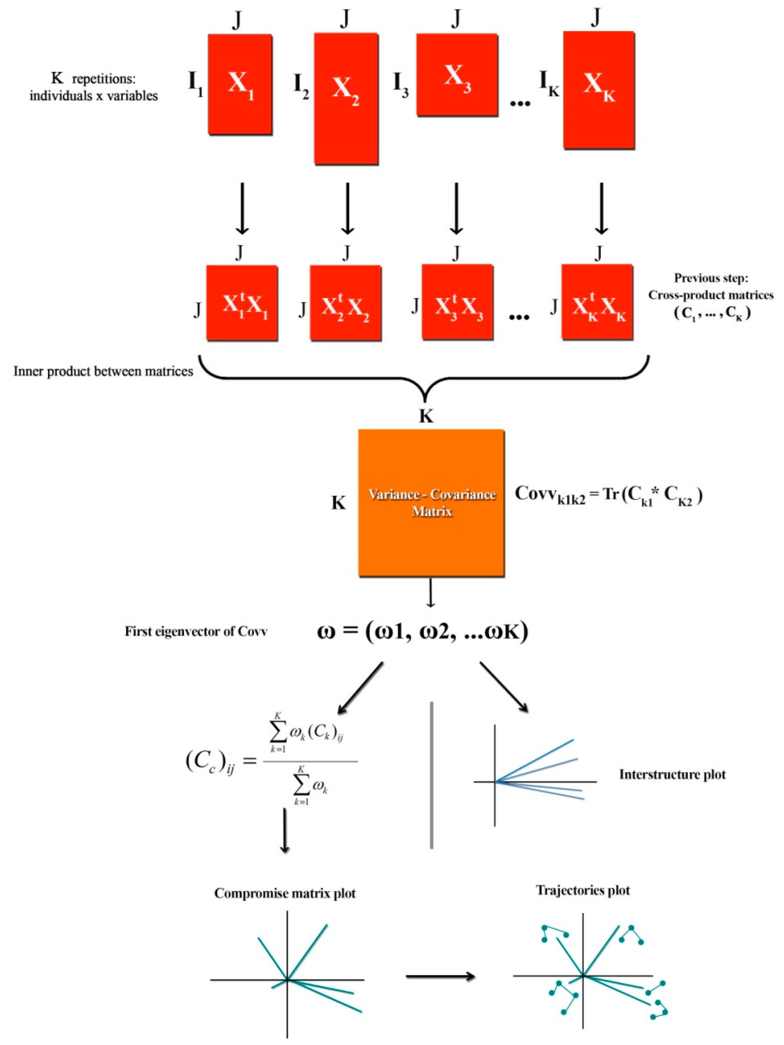
2.2.2. Mathematical Algorithm

Let us define a generic data set as X, where X is a sequence of the matrices X₁, X₂, …, X_K. As we have said before, the different matrices have the same number of columns, J, but they may have other numbers of rows, I₁, I₂, …, I_K. Every X_ijk, where I = 1, 2, …, I_k, j = 1, 2, …, J and k = 1, 2, …, K, can only have two different values: 1 or 0; that is the meaning that our data are dichotomous.

Let us present now the mathematical algorithm of the Dichotomous STATIS DUAL for a generic data set:

1. Previous step: For each X_k, we calculate the average vector (row) v_k as:

$${\left({\mathrm{v}}_{\mathrm{k}}\right)}_{\mathrm{j}}=\frac{1}{{\mathrm{I}}_{\mathrm{k}}}{\displaystyle \sum }_{\mathrm{i}=1}^{{\mathrm{I}}_{\mathrm{k}}}{\mathrm{X}}_{\mathrm{ijk}}$$

(1)

2. For each pair of vectors, we calculate the cosine similarity coefficient, and we build the similarity matrix S, with K rows and K columns:

$${\mathrm{S}}_{{\mathrm{k}}_1{\mathrm{k}}_2}=\frac{{\mathrm{v}}_{{\mathrm{k}}_1}·{\mathrm{v}}_{{\mathrm{k}}_2}}{\Vert {\mathrm{v}}_{{\mathrm{k}}_1}\Vert ·\Vert {\mathrm{v}}_{{\mathrm{k}}_2\Vert }}=\frac{{{\displaystyle \sum }}_{\mathrm{j}=1}^{\mathrm{J}}{\left({\mathrm{v}}_{{\mathrm{k}}_1}\right)}_{\mathrm{j}}{\left({\mathrm{v}}_{{\mathrm{k}}_2}\right)}_{\mathrm{j}}}{\sqrt{{{\displaystyle \sum }}_{\mathrm{j}=1}^{\mathrm{J}}{\left({\mathrm{v}}_{{\mathrm{k}}_1}\right)}_{\mathrm{j}}^2}·\sqrt{{{\displaystyle \sum }}_{\mathrm{j}=1}^{\mathrm{J}}{\left({\mathrm{v}}_{{\mathrm{k}}_2}\right)}_{\mathrm{j}}^2}}$$

(2)

3. We calculate the first eigenvector of the matrix S, namely, ω=(ω₁, ω₂, …, ω_K).

4. We build the compromise vector v_c as:

$${\left({\mathrm{v}}_{\mathrm{c}}\right)}_{\mathrm{j}}=\frac{{{\displaystyle \sum }}_{\mathrm{k}=1}^{\mathrm{K}}{\mathsf{\omega }}_{\mathrm{k}}{\left({\mathrm{v}}_{\mathrm{k}}\right)}_{\mathrm{j}}}{{{\displaystyle \sum }}_{\mathrm{k}=1}^{\mathrm{K}}{\mathsf{\omega }}_{\mathrm{k}}}$$

(3)

5. Final step: We can plot the interstructure employing the ω coefficients, the compromise using the v_c vector, and the trajectories through the v₁, v₂, …, v_K vectors.

Mathematically, the process for the Dichotomous STATIS DUAL method is as follows: for each repetition X_k the average vector v_k is computed; then the cosine similarity coefficient between each pair of average vectors v_k1, v_k2 is computed, which will lead to a matrix built with all the coefficients for every pair of vectors, namely S; then the first eigenvector from the matrix S, ω = (ω₁, …, ω_K), is computed; then the compromise vector is computed as the linear combination of all the average vectors with ω_k as weights, that is, v_c = ω₁*v₁ + … + ω_K*v_K after rescaling the eigenvector to have sum one; moreover, the matrix S can be plotted in a two-dimensional graphic (interstructure), as well as v_c (compromise), even the original v_k can be plotted in the subspace of v_c (intrastructure).

3. Results

3.1. Material and Methods

In this research, we are going to apply this new Dichotomous STATIS DUAL technique to study the learning styles a person can present, namely, four styles or dimensions: activist, reflector, theorist, and pragmatist. The tool we will examine is the CHAEA learning styles test—Cuestionario Honey-Alonso de Estilos de Aprendizaje [21,22]—where each one of the 80 items has to do with one of the four dimensions (see the last four columns in

Table 1. Homogeneous groups obtained from the compromise plot with the learning styles which the items belong to.

Group	Interval of Ratios	Items Belonging to the Group	Learning Styles
			Activist	Reflector	Theorist	Pragmatist
1	<0.5	EA3	1	0	0	0
2	(0.5, 0.6)	EA25, EA37, EA38, EA48, EA62, EA67, EA72, EA74, EA75, A76, EA77	6	0	1	4
3	(0.6, 0.7)	EA5, EA6, EA7, EA13, EA23, EA27, EA28, EA33, EA35, EA39, EA42, EA46, EA47, EA49, EA56, EA58, EA60, EA65, EA68, EA73, EA80	6	6	7	4
4	(0.7, 0.8)	EA1, EA4, EA8, EA10, EA11, EA12, EA14, EA15, EA16, EA17, EA18, EA19, EA20, EA21, EA22, EA24, EA26, EA29, EA30, EA31, EA32, EA34, EA36, EA40, EA41, EA43, EA44, EA50, EA51, EA52, EA53, EA54, EA55, EA57, EA59, EA63, EA64, EA69, EA70, EA71, EA78, EA79	6	14	11	12
5	>0.8	EA2, EA61	1	0	1	0

). ‘Activists’ are people who look for learning through new experiences and are spontaneous and open-minded; ‘reflectors’ are people who know through observation and analysis of situations in addition to their experience; ‘theorists’ are very objective people, and they put aside their beliefs and subjectivity; and ‘pragmatists’ are people who have a very practical but no methodical way of facing situations or solving problems [22].

The sample comprises 1475 randomly chosen university students who answered the 80 items of the CHAEA test. These students belong to different university knowledge areas like Arts and Humanities, Education Sciences, Natural, Exact and Computer Sciences, Health Sciences, Social Sciences, Administration and Law, Engineering, Manufacturing, and Construction or Agronomy and Veterinary Medicine. Data over the years 2014 (340 students), 2015 (478 students), and 2016 (657 students) were available. In addition, we know whether the students are women (728 students) or men (747 students), as well as their age (mean ± standard deviation: 18.389 ± 2.033), which could be very useful if in our study we wanted to analyze the differences that can exist between the learning styles for male or female students, or by age. Although the initial sample comprised more students, some had to be removed due to a lack of data.

Since the answers to the CHAEA learning styles test can only have two different values: 1 or 0, and due to the lack of techniques that analyze data organized like for a STATIS DUAL (a sequence of matrices all of them with the same variables in columns but with different individuals in rows) for those dichotomous items (those with 1 or 0 answers), we can justify that a new proposal must be created to be useful for that and its applicability to real data.

3.2. Interface of the Software

The programming language used to code the Dichotomous STATIS DUAL and the software to implement it was R [21], an environment for statistical computing and graphics.

Although R has a command line interface, several third-party graphical user interfaces exist, such as RStudio, an integrated development environment, or Jupyter, a notebook interface. Four essential features of the RStudio interface can be useful: a space to write the code; a list of all the objects that have been created during the analysis, like the matrix sequence, the names for the different elements or the colors that will be used; a console, that can be used if we wanted to type more commands than the ones on our code; and the different plots that are created after executing the code.

3.3. Commands for the Software

Part of the command sequence comprises externally reading our data, for example, built by mean of a ‘tall’ matrix where the matrices corresponding to each of the years of study are concatenated one below the other. Therefore, this matrix ready to be read from the software will have I₁ + I₂ + ... + I_K rows and J columns. Then, we will have to define which rows correspond to which year.

Other commands will be naming the rows, columns and repetitions of the data as input and defining the colors for the graphical representations. Some of these commands can even be defined in the matrix itself but others have to be read from the keyboard.

Another essential task is to ensure the data are coded as the following: 1 values mean affirmative answers to the variables, while 0 values indicate negative answers. In case our data are differently coded, a command is needed to transform it in the same way.

The next command has to do with the arranging of the data. Although we have already read the data from an external file using a ‘tall’ matrix, we will have to put it in a matrix sequence way, a list of matrices with their rows, columns, and repetitions names.

The final commands are just about the algorithm explained before, corresponding to all the steps needed to perform the Dichotomous STATIS DUAL.

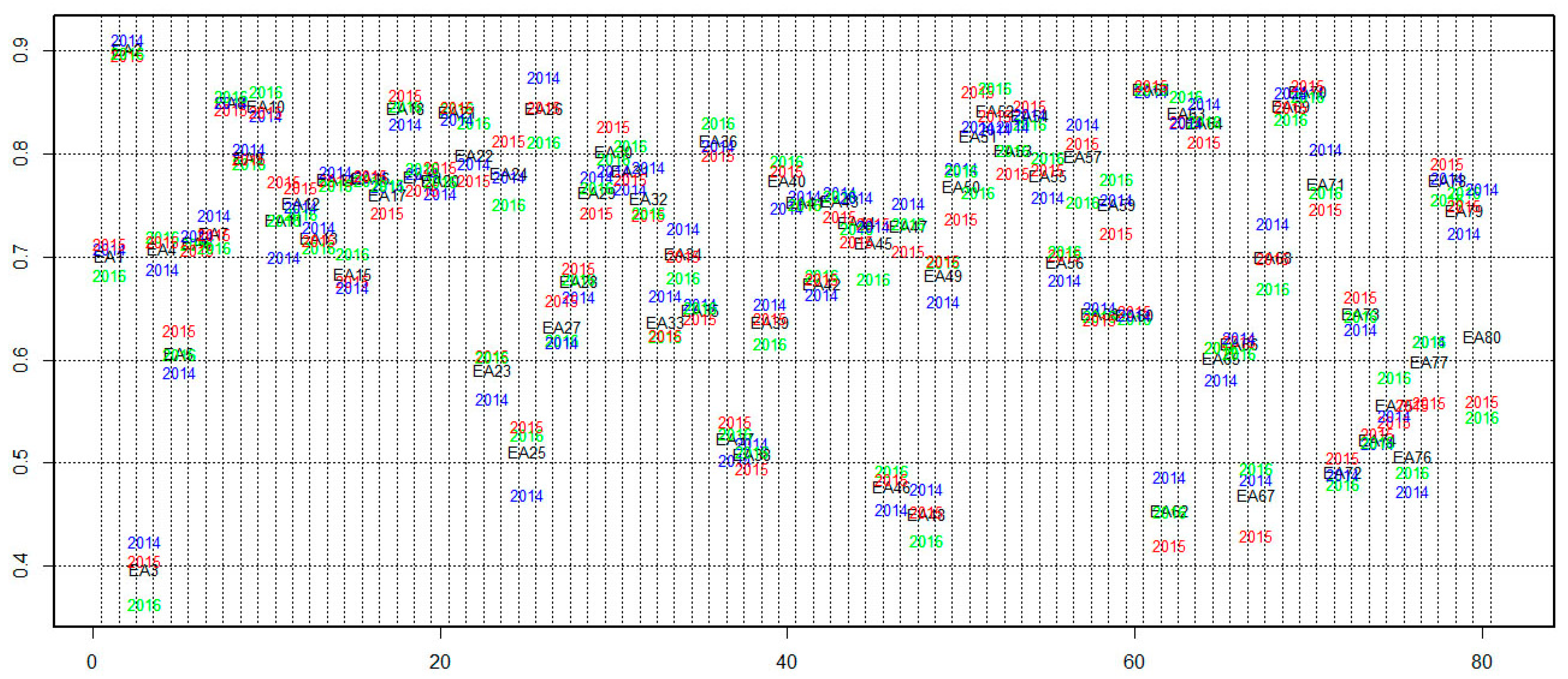
3.4. Results. Example of an Empirical Analysis

After carrying out the Dichotomous STATIS DUAL mathematical algorithm described in the previous section for our sample of the answers that university students gave to all the items from the CHAEA test in order to study their learning styles, the last step of that algorithm is about graphically representing the interstructure, compromise, and trajectories plots as if we were performing a regular STATIS DUAL analysis. In this section, what is represented in each plot is explained because there are slight differences with the ones we obtain after a STATIS DUAL analysis. Moreover, the way these plots can be interpreted will be explained, meaning that we will use our sample as an example of how we can obtain conclusions from the plots.

The first thing we can plot is interstructure. As it has been said in a previous section, this interstructure graphic can be plotted if we calculate the first two eigenvectors of the similarity matrix S, and it can be useful in order to explain the relations between the vectors with the averages for all the rows from every matrix in the sequence. In our case, as the different matrices of the data sequence have the information for each year of study of the answers of the students (by rows) to the CHAEA test items (by columns), that is, their behavior about their learning styles, each one of these vectors has the information of the average values for each item during the corresponding year (2014, 2015 and 2016, respectively).

In Figure 3, we show the interstructure plot, and its interpretation has to do with the angles between all the vectors and the angle separating each vector from the horizontal axis.

The smaller an angle between two vectors is, the more correlated the years they represent will be, that is, the students answered similarly to most of the items during the two years, which means that the predominant learning styles of both years were the same. On the other hand, the closer to a 90-degree angle the two vectors present, the more uncorrelated or independent the years will be, meaning that, for example, the answers the students gave to most of the items in one year are heterogeneous, vary a lot among students, while during the other year the answers were more homogeneous for most of the items, the students were similar, therefore there is no pattern in the answers to the items (that is, no predominant learning styles are found) among years.

Moreover, we could extract conclusions from the angle the vectors present with respect to the horizontal axis: the closer a vector is to this axis (in angle), the more weight it will contribute to the compromise. So, the vectors plotted near the horizontal axis are the ones that are more similar to the rest, generally speaking, while vectors plotted far from this axis will give less weight to the building of the compromise because they are years very different from the others.

Let us interpret our interstructure graphic (Figure 3) according to the previous paragraphs. In our case, the closest vector to the horizontal axis is the one that represents the year 2016; that is, the answers that the students gave to the CHAEA items that year lie on the average of the entire period of three years, while in the other two years (2014 and 2015) the answers were very different from the average, and, in fact, very different from each other: 2015 is plotted below the horizontal axis and 2014 above it. So, the main conclusion is that all the years are very different from each other, where the most considerable difference is between 2014 and 2015, and the average year is similar to 2016.

The next step of the Dichotomous STATIS DUAL is the representation and interpretation of the compromise plot. The compromise graphic is shown in Figure 4, and the interpretation has to do with the following aspects: the horizontal axis represents the number of columns the matrices in the sequence have, in our case, the 80 CHAEA learning styles test items; as our data are dichotomous, all the possible values our matrices have are 0 or 1, where 1 represents an affirmative answer in a specific item and 0 a negative answer, so the vertical axis informs about the ratio of students who answered affirmatively overall. If the dichotomous matrix sequence represents data about presences and absences, the vertical axis is the ratio of presence of some specific factor in the sample that is being studied. Finally, the item labels in the compromise graphic are plotted in the exact place according to the ratio of affirmative answers that have been given to each of the items of the learning styles test, by means of a weighted average according to what happened in the interstructure step, by using as weights the coordinates of the first eigenvector of the similarity matrix S.

(In Figure 4 and Figure 5 and in the Table 1, EA1, EA2, …, EA80, are the labels of the items from the CHAEA learning styles test—Cuestionario Honey-Alonso de Estilos de Aprendizaje [22] ).

Let us explain how we can interpret and obtain conclusions from this compromise plot (Figure 4). We can think of homogeneous groups with similar characteristics if several elements are placed relatively close in the compromise plot, which is also possible for the Dichotomous STATIS DUAL. However, the difference is that two or more variables (columns of the matrix sequence) will form a group, and then we will say they behave in a similar way if they are placed in the same horizontal stripe. More precisely, two or more variables placed in the same stripe will behave in a similar way because their ratio of affirmative answers lies inside the same interval of length 0.1, for example.

Let us clarify this paragraph above with an example of interpretation for our CHAEA test data’s compromise plot. First of all, there would be a one-element group with the item EA3: ‘I often act without considering the possible consequences’ (which belongs to the ‘activist’ dimension), as it is the only item whose ratio of affirmative answers is below 0.5, that is, less than half of the students, on average along the three years, answered ‘yes’ to this item, which means that, although this item belongs to the ‘activist’ dimension, the students who are finally classified as ‘activists’ answered negatively to that item. In the opposite side, there would be a group with two elements, the items EA2: ‘I have strong beliefs about what is right and wrong, good and bad’ (which belongs to the ‘theorist’ dimension) and EA61: ‘When things go wrong, I am happy to shrug it off and “put it down to experience”’ (which belongs to the ‘activist’ dimension), which are the items whose ratios of affirmative answers were above 0.8, meaning that more than 80% of the students answered ‘yes’ to either item; oppositely from the previous item conclusions, most of the students will be finally classified as ‘theorists’ or ‘activists’, respectively, if they answered positively to those items.

Between these lower and higher groups, we could find another three (see Table 1): the first one, with 11 items, whose ratios take values ranging from 0.5 to 0.6; the second one, with 23 items, whose ratios take values ranging from 0.6 to 0.7; and the third one, with most of the items of our data (43 items), whose ratios take values ranging from 0.7 to 0.8. Let us speak a bit about these homogeneous groups between the lowest and the highest groups: the first one (11 items) is more related to the ‘activist’ learning style because 6 out of 11 items belong to that dimension; the most predominant learning style in the second one (23 items) is the ‘theorist’ because of the 7 items that belong to that dimension, and the third one (43 items) is more related to the ‘reflector’ dimensions thanks to the 14 out of 43 items that belong to that learning style.

If we wanted to extract more specific conclusions, we could change the width of the horizontal stripes, that is, create shorter intervals for the ratios, with length 0.05, for example, to find more homogeneous groups of items.

The last step of the Dichotomous STATIS DUAL is the representation and interpretation of the intrastructure, also known as trajectories, where, oppositely to the compromise analysis that studied the average behavior of the matrices in the sequence, the intrastructure studies how the columns evolve along the years, that is, the real differences between the points in the compromise plot that represent the average columns and the points that represent the columns according to every year. Therefore, we will plot in the same graphic the points from the compromise graphic and the points for the intrastructure (Figure 5), what can be done because, mathematically, the original data from all the sequence matrices can be projected to the plane obtained to plot the compromise analysis.

The way to interpret this intrastructure plot is similar to the compromise plot. We could think of which groups of columns (in our case, the CHAEA learning styles test items) can be formed according to which stripe they belong to, with the difference that now we are not taking into account just the average matrix from the sequence (the average year in our case) but all the matrices of study (all the years). We can speak about during which repetition which items have ratios of affirmative answers (or ratios of presences of factors) higher or lower than the other repetitions or the average matrix. Moreover, we can also mention which columns have more variability along the studied period by observing how widely spread the repetitions are placed around the point representing the average column from the compromise analysis.

As an example of the interpretation of this intrastructure plot according to the previous paragraph, we will speak here about a couple of items and their behavior in Figure 5. Let us interpret items EA37: ‘Quiet, thoughtful people tend to make me feel uneasy’ and EA78: ‘I like meetings to be run on methodical lines, sticking to laid down agenda’.

If we focus on item EA37, which belongs to group 2 (Table 1). In that case, the average year has a value of the ratio of affirmative answers between 0.5 and 0.6 (near 0.57), but we can see an evolution along the years: during 2014, the ratio was similar to the average; then, during 2015 the ratio fell until a value near 0.53; and finally, during 2016 the ratio grew up until a much higher value even above 0.6; so, the main conclusion is that EA37 varies a lot along the years: much fewer ‘yes’ answers were given during 2015 than during 2014, and much more ‘yes’ answers were given during 2016.

Now, if we focus on item EA78, which belongs to group 4 (see Table 1, the ratio between 0.7 and 0.8), the average year and the three years 2014, 2015, and 2016 have very similar values, and the evolution in this case was much lower than the rest of the items from our data: the ratio of students who answered ‘yes’ to this item barely changed.

4. Discussion

There are not many multivariate statistical techniques or software for the analysis of dichotomous data, and even less if they represent different instances of time arranged in a sequence of matrices that must be analyzed, or matrices with a different number of individuals, as the particular case of this research. We can currently find many studies that have dichotomous information but are not appropriately analyzed because of the lack of techniques that allow a better result; as it is the case of the study by Tejedor Flores (2016), where he talks about the global reporting initiative (GRI) of Brazilian companies sorted according to their economic, social and environmental components during the years 2011, 2012 and 2013 with the aim of knowing the trends and habits of sustainability reports of Brazilian companies [23] and the study by Cañizares et al. (2016) where germplasm data of a local corn variety are addressed through SSR markers [24]; as a result of this, valuable information is lost, and decisions are made with a more significant margin of error.

The interesting things about these techniques are the needs and gaps that still exist in science, so much which they have had to be developed in areas very different from the statistical or mathematical branches, like examples in gastronomic, ecological or biological contexts, that came to satisfy those needs of information, which is an interesting issue because despite the lack of a technique that allows the analysis, authors chose to limit themselves to only using the chi-squared test [25], the analysis of the variance ANOVA [25,26] and the normality and homoscedasticity tests [25].

Dichotomous data need a specific technique different from the existing ones for multiblock data, so a proposal called DICHOTOMOUS STATIS DUAL is made as an alternative for a more efficient analysis of dichotomous data from multiple tables, in particular for a sequence of matrices—all of them with the same variables in columns but with different individuals in rows. We can justify that a new proposal must be created to be useful for that and its applicability to real data due to the lack of a specific technique for dichotomous data.

Another predecessor proposal is the technique called CATATIS, which focuses on the study of dichotomous data, but with the particularity one must have the same rows and columns on all the occasions.

According to the information found in the above-mentioned studies about the lack of a methodology that allows studying information for a long time with dichotomous data, we presented our proposal seeking to satisfy the need of a statistical method that would meet the characteristics required by our data (different rows and same columns at different times) and having the STATIS family methods as a background. The new Dichotomous STATIS DUAL technique is an alternative multivariate data analysis method with applicability in all areas of knowledge, thanks to the software presented in this research. We consider the Dichotomous STATIS DUAL method and the corresponding algorithm suitable for establishing a new proposal that would allow us to interpret the dichotomous data from a sequence of matrices more logically. The advantages of using the new proposal for sequences of dichotomous matrices presented in this work became evident.

Finally, a description of the main types of information extracted from the use of the method proposed is presented: with the interstructure analysis the information we can extract is about how different or similar the behavior of the patterns in the answers to the variables was along the repetitions; then, with the compromise plot, the information we can extract is about the average behavior of the patterns in the answers along the repetitions, that is, the common structure in the data along the third dimension; while with the intrastructure plot, the information we can extract is about how the answers that the individuals gave to the variables vary along the repetitions, that is, how the third dimension influences so it can make that common structure not so stable but dynamic.

Therefore, derived from the analysis of the literature and due to the lack of a method that allows analyzing dichotomous data over time, this new multivariate technique is proposed to take full advantage of data bases, especially those that are longitudinal in nature and make more complete and functional analysis.

References

1. L’Hermier des Plantes, H. Structuration Des Tableaux à Trois Indices de La Statistique. Ph.D. Thesis, Université de Montpellier II, Montpellier, France, 1976. [Google Scholar]
2. Jaffrenou, P.-A. Sur l’analyse Des Familles Finies de Variables Vectorielles: Bases Algébriques et Application à La Description Statistique. Ph.D. Thesis, l’Université de Sainte-Etiene, Saint-Étienne, France, 1978. [Google Scholar]
3. Thioulouse, J. Simultaneous Analysis of a Sequence of Paired Ecological Tables: A Comparison of Several Methods. Ann. Appl. Stat. 2011, 5, 2300–2325. [Google Scholar] [CrossRef] [Green Version]
4. Vivien, M.; Sabatier, R. A Generalization of STATIS-ACT Strategy: DO-ACT for Two Multiblocks Tables. Comput. Stat. Data Anal. 2004, 46, 155–171. [Google Scholar] [CrossRef]
5. Sauzay, L.; Hanafi, M.; Qannari, E.M.; Schlich, P. Analyse de K+ 1 Tableauxa l’aide de La Méthode STATIS: Application En Évaluation Sensorielle, 9ieme Journées Européennes Agro-Industrie et Méthodes Statistiques; Société Française de Statistique (SFdS): Montpellier, France, 2006. [Google Scholar]
6. Abdi, H.; Valentin, D.; Chollet, S.; Chrea, C. Analyzing Assessors and Products in Sorting Tasks: DISTATIS, Theory and Applications. Food Qual. Prefer. 2007, 18, 627–640. [Google Scholar] [CrossRef]
7. Vallejo-Arboleda, A.; Vicente-Villardón, J.L.; Galindo-Villardón, M.P. Canonical STATIS: Biplot Analysis of Multi-Table Group Structured Data Based on STATIS-ACT Methodology. Comput. Stat. Data Anal. 2007, 51, 4193–4205. [Google Scholar] [CrossRef]
8. Sabatier, R.; Vivien, M. A New Linear Method for Analyzing Four-Way Multiblock Tables: STATIS-4. J. Chemom. 2008, 22, 399–407. [Google Scholar] [CrossRef]
9. Marcondes Filho, D.; Fogliatto, F.S.; Oliveira, L.P.L.D. Gráficos de controle multivariados para monitoramento de processos não lineares em bateladas. Production 2011, 21, 132–148. [Google Scholar] [CrossRef] [Green Version]
10. Thioulouse, J.; Simier, M.; Chessel, D. Simultaneous Analysis of a Sequence of Paired Ecological Tables. Ecology 2004, 85, 272–283. [Google Scholar] [CrossRef]
11. Bénasséni, J.; Bennani Dosse, M. Analyzing Multiset Data by the Power STATIS-ACT Method. Adv. Data Anal. Classif. 2012, 6, 49–65. [Google Scholar] [CrossRef]
12. Sabatier, R.; Vivien, M.; Reynès, C. Une nouvelle proposition, l’Analyse Discriminante Multitableaux: STATIS-LDA. J. Société Fr. Stat. 2013, 154, 31–43. [Google Scholar]
13. Corrales, D.; Rodríguez, O. Interstatis: The Statis Method for Interval Valued Data. Rev. Matemática Teoría Apl. 2014, 21, 73–83. [Google Scholar] [CrossRef] [Green Version]
14. Kriegsman, M.A. Discriminant Distatis: A Multi-Way Discriminant Analysis for Distance Matrices, Illustrations with the Sorting Task. Ph.D. Thesis, University of Texas, Dallas, TX, USA, 2018. [Google Scholar]
15. Llobell, F.; Cariou, V.; Vigneau, E.; Labenne, A.; Qannari, E.M. A New Approach for the Analysis of Data and the Clustering of Subjects in a CATA Experiment. Food Qual. Prefer. 2019, 72, 31–39. [Google Scholar] [CrossRef]
16. Mérigot, B.; Gaertner, J.-C.; Brind’amour, A.; Carbonara, P.; Esteban, A.; Garcia-Ruiz, C.; Gristina, M.; Imzilen, T.; Jadaud, A.; Joksimovic, A.; et al. Stability of the Relationships among Demersal Fish Assemblages and Environmental-Trawling Drivers at Large Spatio-Temporal Scales in the Northern Mediterranean Sea. Sci. Mar. 2019, 83 (Suppl. S1), 153–163. [Google Scholar] [CrossRef] [Green Version]
17. Llobell, F.; Cariou, V.; Vigneau, E.; Labenne, A.; Qannari, E.M. Analysis and Clustering of Multiblock Datasets by Means of the STATIS and CLUSTATIS Methods. Application to Sensometrics. Food Qual. Prefer. 2020, 79, 103520. [Google Scholar] [CrossRef]
18. Lavit, C. Analyse Conjointe de Tableaux Quantitatifs; Masson: Paris, France, 1988. [Google Scholar]
19. Robert, P.; Escoufier, Y. A Unifying Tool for Linear Multivariate Statistical Methods: The RV-Coefficient. J. R. Stat. Soc. Ser. C Appl. Stat. 1976, 25, 257–265. [Google Scholar] [CrossRef]
20. Ochiai, A. Zoogeographic studies on the soleoid fishes found in Japan and its neighbouring regions. Bull. Jpn. Soc. Sci. Fish. 1957, 22, 526–530. [Google Scholar] [CrossRef] [Green Version]
21. Alonso, C.; Gallego, D.; Honey, Y. Cuestionario Honey-Alonso de Estilos de Aprendizaje. Procedimientos de Diagnósticos y Mejora; Ediciones Mensajero: Bilbao, Spain, 1994. [Google Scholar]
22. RStudio Team. RStudio: Integrated Development for R. RStudio. PBC: Boston, MA, USA, 2020. Available online: http://www.rstudio.com/ (accessed on 3 May 2021).
23. Flores, N.D.T. Análisis Multivariante de la Sostenibilidad a través del Global Reporting Initiative (GRI), Utilizando como Caso de Estudio: Brasil. In Proceedings of the Congreso Internacional De Investigación E Innovación 2016, Guanajuato, Mexico, 21–22 April 2016; p. 6. [Google Scholar]
24. Cañizares, J.F.R.; Abarca, E.F.G.; Naranjo, D.N.C.; Vicente-Villardón, J.L.; Demey, J. Caracterización de germoplasma de maíz local a través de marcadores SSR asistido por biplot logístico externo (BLE). In Proceedings of the XXVI Simposio Internacional de Estadística 2016, Sincelejo, Colombia, 8–12 August 2016; p. 4. [Google Scholar]
25. Rodríguez, H.d.J.D.; Limón, J.A.G.; Pisfil, M.L.; Torres, D.V.; Exume, J.C.D. Estilos de aprendizaje: Un estudio diagnóstico en el centro universitario de ciencias económico-administrativas de la U de G*. Rev. Educ. Super. 2015, 44, 121–140. [Google Scholar] [CrossRef] [Green Version]
26. Viloria, A.; Petro Gonzalez, I.R.; Pineda Lezama, O.B. Learning Style Preferences of College Students Using Big Data. Procedia Comput. Sci. 2019, 160, 461–466. [Google Scholar] [CrossRef]
Figure 1. STATIS DUAL flow chart.
Mathematics 09 02797 g001
Figure 2. Dichotomous STATIS DUAL flow chart.
Mathematics 09 02797 g002
Figure 3. Interstructure plot.
Mathematics 09 02797 g003
Figure 4. Compromise plot.
Mathematics 09 02797 g004
Figure 5. Intrastructure plot.
Mathematics 09 02797 g005