Artificial Intelligence for Stability Control of Actuated In–Wheel Electric Vehicles with CarSim^® Validation

Abstract

This paper presents an active controller for electric vehicles in which active front steering and torque vectoring are control actions combined to improve the vehicle driving safety. The electric powertrain consists of four independent in–wheel electric motors situated on each corner. The control approach relies on an inverse optimal controller based on a neural network identifier of the vehicle plant. Moreover, to minimize the number of sensors needed for control purposes, the authors present a discrete–time reduced–order state observer for the estimation of vehicle lateral and roll dynamics. The use of a neural network identifier presents some interesting advantages. Notably, unlike standard strategies, the proposed approach avoids the use of tire lateral forces or Pacejka’s tire parameters. In fact, the neural identification provides an input–affine model in which these quantities are absorbed by neural synaptic weights adapted online by an extended Kalman filter. From a practical standpoint, this eliminates the need of additional sensors, model tuning, or estimation stages. In addition, the yaw angle command given by the controller is converted into electric motor torques in order to ensure safe driving conditions. The mathematical models used to describe the electric machines are able to reproduce the dynamic behavior of Elaphe M700 in–wheel electric motors. Finally, quality and performances of the proposed control strategy are discussed in simulation, using a CarSim^® full vehicle model running through a double–lane change maneuver.

1. Introduction

The automotive industry is facing an ongoing evolution towards electrification and inclusion of so–called smart features. In these efforts, the use of x–by–wire systems is a common goal. Technologies such as electric power steering [1], electro–hydraulic brakes [2] and regenerative dampers [3] have demonstrated to yield favorable performance and augmented controllable features in automotive systems. As specified by Mazzilli et al. [4], the presence of multiple actuators is conducive to their coordination. This is commonly referred to as Integrated Chassis Control (ICC). In this paradigm, automotive systems pursue five main features: adaptability, fault tolerance, dynamic reconfigurability, modularity and low computational power.

To enable ICC, Ivanov and Savitski [5] highlighted improvements in longitudinal dynamics, lateral dynamics and body motion control. Improvements in these three domains favor vehicle stability, vehicle handling and passenger ride quality. Furthermore, chassis and powertrain electrification also play a major role in this context. Zhang and Zhao proposed a decoupling strategy to decompose steering and driving contributions for an in–wheel powertrain vehicle and provide ICC [6]. More recently, torque optimization strategies with focus on regenerative braking and energy efficiency have been explored [7,8].

In their recent systematic review, Mazzilli et al. [4] found that most of the ICC implementations target the enhancement of lateral vehicle dynamics through improved utilization of the tire–road friction potential. In fact, this sole aspect emphasizes the importance of lateral dynamics in vehicle stability. To provide improved grip and handling, the so–called torque vectoring (TV) strategies yield optimal torque references to each wheel of the vehicle. Since the contact between the tire and the ground plays a fundamental role in propulsion and vehicle stability, previous efforts have focused on the estimation of the tire side–slip angle [9,10]. Many of these works assume the full knowledge of lateral tire forces, which, from a practical standpoint requires dedicated sensors and/or estimation strategies.

In this context, this work combines active front steering (AFS) and TV approaches to improve stability for a vehicle equipped with in–wheel electric motors. The vehicle roll dynamics are here considered non–negligible and a discrete–time reduced–order observer is used to reconstruct the otherwise unknown vehicle lateral and roll dynamics [11,12]. The main contribution of this work consists in the use of a recurrent high–order neural network (RHONN) to identify the vehicle observed dynamics [13,14,15]. The RHONN weight updating process is trained using an extended Kalman filter (EKF). The obtained parameters are then used in the vehicle model to design the control algorithm, in this case, an inverse optimal control. With the RHONN–based model, the AFS input appears linearly in the dynamics and not implicitly in the tire characteristic [16]. This artificial intelligence (AI) approach allows us to calculate the AFS input without inverting the tire model, which is not a trivial task due to the complexity of the tire model and its dependence on the vehicle dynamics. In addition, the TV control law does not depend on an explicit expression of the lateral front and rear tire forces. These quantities are usually not available and they should be estimated. These two aspects, together with the provided stability demonstration, are key aspects covered in this work.

Another aspect worth mentioning is that the proposed controller is determined using the inverse optimal control technique [14,15]. In a classical optimal control setting, the meaningful cost functional is given a priori. Subsequently, it is used to calculate the control law by solving a Hamilton–Jacobi–Bellmann (HJB) equation. In general, this latter task introduces a further challenge. The inverse optimal control technique can be used to overcome this problem, by choosing an a priori candidate Lyapunov function, which is then used to calculate the control law and a meaningful cost functional [14,15].

To validate the described approach, CarSim^® [17] is the tool of choice. This software provides custom parametric mathematical models for full dynamics, which feature lightweight but accurate representations of a real vehicle. CarSim^®  is an automotive industry standard since 1990. Moreover, its seamless integration with MATLAB/Simulink^®  allows users to validate different control strategies through co–simulation.

This work is organized as follows: Section 2 presents the proposed control method applied to a ground vehicle with roll dynamics, where the reduced–order state observer, neural model and control laws are described. Section 3 shows the simulation results obtained by using the CarSim^®full vehicle model for an interesting case in which the vehicle performs a double–lane change (DLC) maneuver under an abrupt variation of the tire–road friction coefficient. Finally, Section 4 concludes the work and opens the possibility to future works.

2. Neural Network Inverse Optimal Control for In–Wheel Electric Vehicles

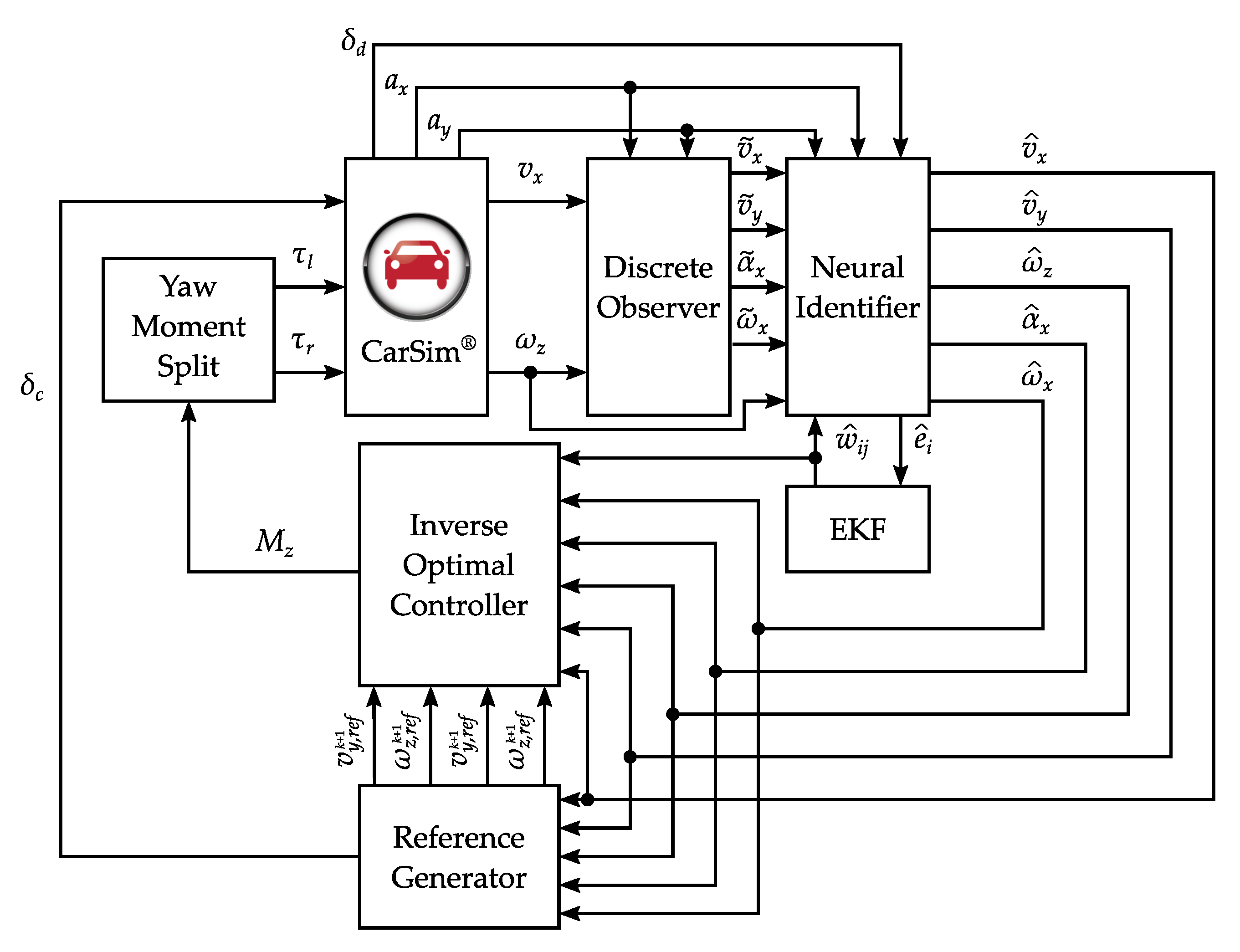
For a better understanding of the control purposes, Figure 1 shows the control scheme utilized in this work. The signals measured from the CarSim^® plant are the steering wheel angle ${\delta }_{d,k}$ and the longitudinal and lateral vehicle accelerations $a_{x,k}$ and $a_{y,k}$, as well as the longitudinal vehicle speed $v_{x,k}$ and the yaw rate ${\omega }_{z,k}$. Then, a discrete–time reduced–order state observer provides estimation of vehicle lateral velocity ${\tilde{v}}_{y,k}$, roll position ${\tilde{\alpha }}_{x,k}$ and velocity ${\tilde{\omega }}_{x,k}$. Next, measured and observed dynamics are given to the neural identifier as input. By using synaptic weights trained in an EKF, the neural identifier is able to provide an input–affine neural model that approximates the vehicle plant model.

Subsequently, the inverse optimal controller, based on the neural model, ensures asymptotic stability of the desired references given for the vehicle lateral velocity $v_{y,k,\mathrm{ref}}$ and yaw rate ${\omega }_{z,k,\mathrm{ref}}$. Outputs of the controller are the active front steering (AFS) and the torque vectoring (TV), named ${\delta }_{c,k}$ and $M_{z,k}$, respectively. The AFS is directly given as control feedback to the vehicle plant model, whereas the TV is split into two different components, namely, the electric motor torques to be given to the left and right side of the powertrain, ${\tau }_{l,k}$ and ${\tau }_{r,k}$, respectively.

2.1. The Vehicle Mathematical Model with Roll Dynamics

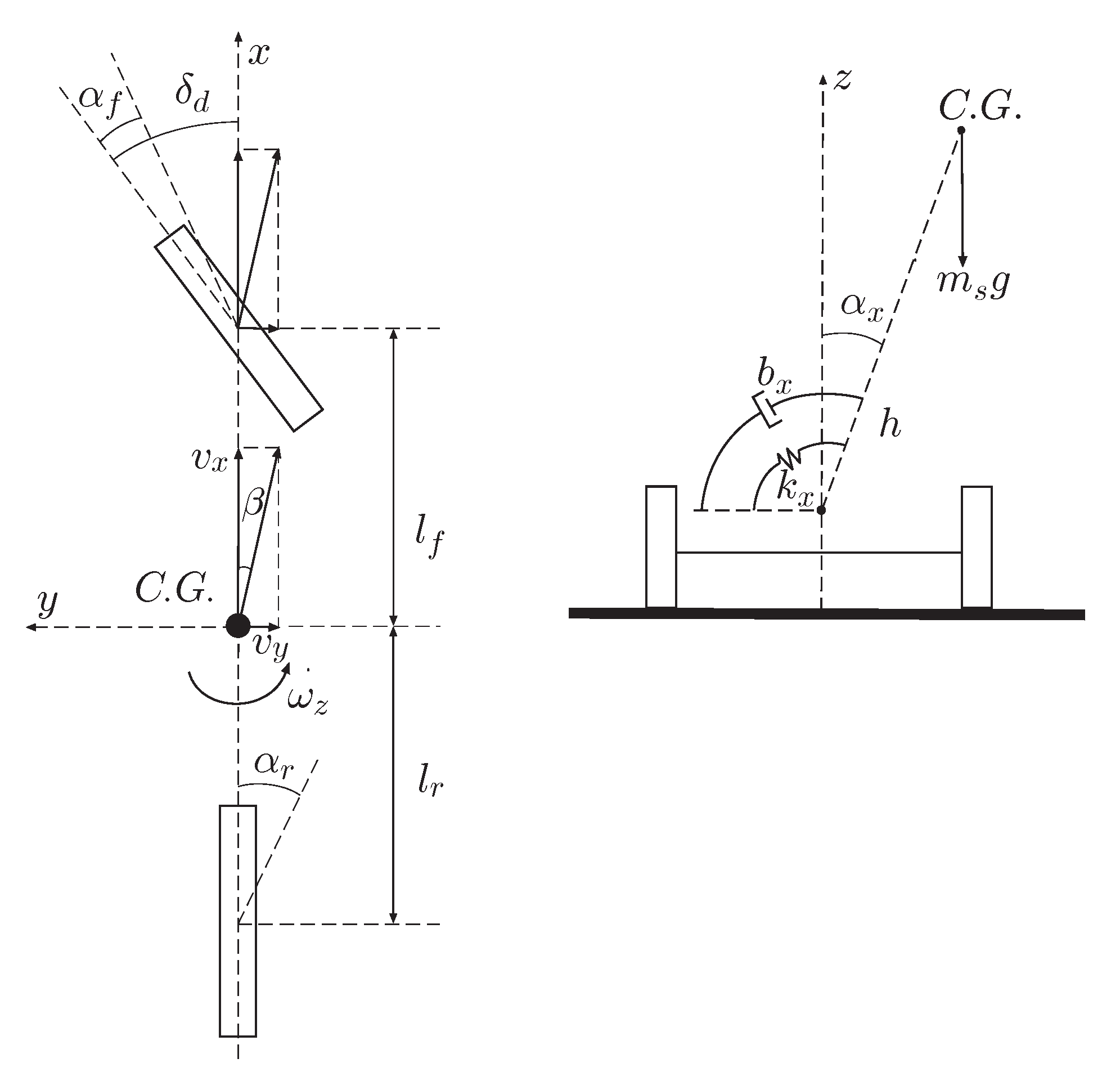
For vehicles with generic center of gravity height, the essential dynamics describing the vehicle attitude are given by the longitudinal and lateral velocities, the yaw rate and the roll dynamics. The latter, if not considered, can generate vehicle instability as explained in [11,12]. To this aim, the vehicle mathematical model including roll dynamics is well described by the bicycle model in Figure 2. This representation is often used to design active controllers for ground vehicles [18,19,20].

The interested reader can find, in [21], a discrete–time version of such a model, obtained by means of a variational integrator (known as symplectic Euler) and representing the discrete–time version of the bicycle model. Although this model ensures better performance for (relatively) high sampling periods, a more popular model is the Euler approximation.

$$\left(\begin{array}{c}{v}_{x,k+1}\\ v_{y,k+1}\\ {\omega }_{z,k+1}\\ {\alpha }_{x,k+1}\\ {\omega }_{x,k+1}\end{array}\right)=(\begin{array}{c}{v}_{x,k}+T(v_{y,k}{\omega }_{z,k}+a_{x,k}-\frac{m_{s}h}{m}{\omega }_{z,k}{\omega }_{x,k})\\ v_{y,k}+T(-v_{y,k}{\omega }_{z,k}+\frac{1}{m_e}{a}_{y,k}-\frac{k_{x,e}}{J_{x,s}}{\alpha }_{x,k}-\frac{b_x}{J_{x,s}}{\omega }_{x,k})\\ {\omega }_{z,k}+T\left(\frac{{\mu }_y}{J_z}\right(F_{y,f}\left({\alpha }_{f,k}\right)l_f-F_{y,r}\left({\alpha }_{r,k}\right)l_r)+\frac{M_z}{Jz})\\ {\alpha }_{x,k}+T{\omega }_{x,k}\\ {\omega }_{x,k}+T(\frac{m_{s}h}{J_{x,e}}{a}_{y,k}-\frac{k_{x,e}}{J_{x,e}}{\alpha }_{x,k}-\frac{b_x}{J_{x,e}}{\omega }_{x,k})\end{array})$$

(1)

where T is the sampling period; $v_{x,k}$, $v_{y,k}$ and ${\omega }_{z,k}$ are the vehicle longitudinal, lateral and yaw velocities; ${\alpha }_{x,k}$ and ${\omega }_{x,k}$ are the roll position and velocity, respectively. The longitudinal acceleration can be expressed as

$$a_{x,k}={\displaystyle \frac{{\mu }_x}{m}}\left(F_{x,f}\left({\lambda }_{f,k}\right)+F_{x,r}\left({\lambda }_{r,k}\right)\right)$$

where $F_{x,f}$ and $F_{x,r}$ are the longitudinal forces, depending on the front/rear tire slips ${\lambda }_{f,k}=1-{\omega }_{w,f,k}{R}_w/v_{x,k}$, ${\lambda }_{r,k}=1-{\omega }_{w,r,k}{R}_w/v_{x,k}$ (where ${\omega }_{w,f,k}$ and ${\omega }_{w,r,k}$ are the front/rear wheel angular velocities) and $R_w$ is the wheel radius.

The lateral acceleration is given by

$$a_{y,k}={\displaystyle \frac{{\mu }_y}{m}}\left(F_{y,f}\left({\alpha }_{f,k}\right)+F_{y,r}\left({\alpha }_{r,k}\right)\right)$$

where $F_{y,f}$ and $F_{y,r}$ are the lateral forces which depend on the tire slip angles ${\alpha }_{f,k}={\delta }_{d,k}+{\delta }_{c,k}-(v_{y,k}+l_f{\omega }_{z,k})/v_{x,k}$ and ${\alpha }_{r,k}=-(v_{y,k}-l_r{\omega }_{z,k})/v_{x,k}$ (where ${\delta }_{d,k}$ is the driver steering wheel angle and ${\delta }_{c,k}$ is the AFS input).

As previously stated, this work does not rely on a specific tire model. The only assumption, verified in practice, is that the tire characteristics are bounded functions [16]. For the sake of concreteness, one may consider, for instance, a simplified Pacejka’s model for the longitudinal and lateral forces.

$$F_{i,j}=D_{i,j}sin\left(C_{i,j}arctan{B}_{i,j}{\alpha }_j\right)$$

with $i=x,y$ and $j=f,f$ and where the constants $D_{i,j}$, $C_{i,j}$ and $B_{i,j}$ are experimentally determined.

Finally, m and $J_z$ are the vehicle mass and inertia momentum; $l_f$ and $l_r$ are the front and rear vehicle length; and ${\mu }_x$ and ${\mu }_y$ are the longitudinal and lateral tire–road friction coefficients. Furthermore, $M_{z,k}$ is the TV input.

2.2. The Control Problem

As already mentioned, the use of the AFS and the TV allows us to track given references for the lateral velocity $v_{y,k,\mathrm{ref}}$ and the yaw rate ${\omega }_{z,k,\mathrm{ref}}$.

Thus, the control problem can be defined as follows: given bounded references $v_{y,k,\mathrm{ref}}$ and ${\omega }_{z,k,\mathrm{ref}}$, with bounded increments, determine a controller $u_k={\alpha }_k({\widehat{x}}_k,x_{k,\mathrm{ref}})$, such that the tracking errors $e_{v_{y,k}}=v_{y,k}-v_{y,k,\mathrm{ref}}$, $e_{{\omega }_{z,k}}={\omega }_{z,k}-{\omega }_{z,k,\mathrm{ref}}$ satisfy

$$\underset{k\to \infty }{lim}{e}_{v_{y,k}}=0,\underset{k\to \infty }{lim}{e}_{{\omega }_{z,k}}=0.$$

Moreover, when applying control strategies for vehicle stability, not all the state measurements are available. To avoid an extensive use of sensors, we present a discrete–time reduced–order state observer for the reconstruction of the vehicle lateral velocity ${\tilde{v}}_{y,k}$, roll position ${\tilde{\alpha }}_{x,k}$ and velocity ${\tilde{\omega }}_{x,k}$.

Making reference to Figure 1, the tracking errors $e_{v_{y,k}}$ and $e_{{\omega }_{z,k}}$ can then be bounded as follows:

$$\begin{array}{cc}\hfill \parallel e_{v_{y,k}}\parallel & \le \parallel v_{y,k}-{\tilde{v}}_{y,k}\parallel +\parallel {\tilde{v}}_{y,k}-{\widehat{v}}_{y,k}\parallel +\parallel {\widehat{v}}_{y,k}-v_{y,k,\mathrm{ref}}\parallel \hfill \\ \hfill \parallel e_{{\omega }_{z,k}}\parallel & \le \parallel {\omega }_{z,k}-{\widehat{\omega }}_{z,k}\parallel +\parallel {\widehat{\omega }}_{z,k}-{\omega }_{z,k,\mathrm{ref}}\parallel .\hfill \end{array}$$

Thus, the tracking problem of desired trajectories can be split into three requirements:

• $\underset{k\to \infty }{lim}\parallel v_{x,k}-{\tilde{v}}_{x,k}\parallel =0$; $\underset{k\to \infty }{lim}\parallel v_{y,k}-{\tilde{v}}_{y,k}\parallel =0$
• $\underset{k\to \infty }{lim}\parallel {\tilde{v}}_{x,k}-{\widehat{v}}_{x,k}\parallel \le {\epsilon }_{e_1}$, $\underset{k\to \infty }{lim}\parallel {\tilde{v}}_{y,k}-{\widehat{v}}_{y,k}\parallel \le {\epsilon }_{e_2}$, $\underset{k\to \infty }{lim}\parallel {\omega }_{z,k}-{\widehat{\omega }}_{z,k}\parallel \le {\epsilon }_{e_3}$,
  $\underset{k\to \infty }{lim}\parallel {\tilde{\alpha }}_{x,k}-{\widehat{\alpha }}_{x,k}\parallel \le {\epsilon }_{e_4}$, $\underset{k\to \infty }{lim}\parallel {\tilde{\omega }}_{x,k}-{\widehat{\omega }}_{x,k}\parallel \le {\epsilon }_{e_5}$
  ;
• $\underset{k\to \infty }{lim}\parallel {\widehat{v}}_{y,k}-v_{y,k,\mathrm{ref}}\parallel =0$, $\underset{k\to \infty }{lim}\parallel {\widehat{\omega }}_{z,k}-{\omega }_{z,k,\mathrm{ref}}\parallel =0$.

where ${\epsilon }_{e_i}>0$$\forall i=1,\cdots ,5$ are fixed bounds for the norm of the identification errors.

The asymptotic stability of the estimation error stated in the first condition is ensured by the use of a reduced–order state observer, as presented in Section 2.4. The practical stability of the identification error required by the second condition is guaranteed by using the RHONN identifier introduced in Section 2.5. In addition, the reference tracking stability required by the third condition is satisfied by the utilization of the discrete–time controller discussed in Section 2.6, developed with the inverse optimal control technique. Before these conditions are met, Section 2.3 shows how to generate safe references for the vehicle attitude.

2.3. The Reference Signals

The references $v_{y,k,\mathrm{ref}}$ and ${\omega }_{z,k,\mathrm{ref}}$ represent what the driver expects from the vehicle performance. No reference is imposed on $v_{x,k}$. This work assumes that the slips ${\lambda }_{f,k}$ and ${\lambda }_{r,k}$ are set to zero; therefore, no longitudinal acceleration/deceleration is imposed. Various expressions can be found in the literature as reference generators. In particular, we consider—without loss of generality—the references given in [11,12] as the behavior of an “ideal” or “reference” vehicle. This ideal vehicle is not controlled by the AFS and/or the TV and receives, as input, only the driver’s steering signal.

$$\left(\begin{array}{c}{v}_{y,k+1,\mathrm{ref}}\\ {\omega }_{z,k+1,\mathrm{ref}}\end{array}\right)=\left(\begin{array}{c}{v}_{y,k,\mathrm{ref}}-T{v}_{x,k}{\omega }_{z,k,\mathrm{ref}}+\\ T\frac{{\mu }_{y,\mathrm{ref}}}{m_{\mathrm{ref}}}\left(F_{y,f,\mathrm{ref}}\right({\alpha }_{f,\mathrm{ref}})+F_{y,f,\mathrm{ref}}({\alpha }_{r,\mathrm{ref}}\left)\right)\\ {\omega }_{z,k,\mathrm{ref}}+T\frac{{\mu }_{y,\mathrm{ref}}}{J_{z,\mathrm{ref}}}\left(F_{y,f,\mathrm{ref}}\right({\alpha }_{f,\mathrm{ref}})l_f-F_{y,f,\mathrm{ref}}({\alpha }_{r,\mathrm{ref}}\left)l_f\right)\end{array}\right)$$

(2)

The reference lateral forces $F_{y,f,\mathrm{ref}}$ and $F_{y,r,\mathrm{ref}}$ depend on the reference slip angles

$${\displaystyle \phantom{(}{\alpha }_{f,\mathrm{ref}}={\delta }_{d,k}-\frac{v_{y,k,\mathrm{ref}}+l_f{\omega }_{z,k,\mathrm{ref}}}{v_{x,k}},{\alpha }_{r,\mathrm{ref}}=-\frac{v_{y,k,\mathrm{ref}}-l_r{\omega }_{z,k,\mathrm{ref}}}{v_{x,k}}}$$

(3)

and appear multiplied by the reference lateral tire–road friction coefficient ${\mu }_{y,\mathrm{ref}}$. These reference forces $F_{y,f,\mathrm{ref}}$ and $F_{y,r,\mathrm{ref}}$ are determined using the Pacejka’s Magic Formula [16]

$$F_{y,i,\mathrm{ref}}=D_{y,i,\mathrm{ref}}sin(C_{y,i,\mathrm{ref}}arctan\left(B_{y,i,\mathrm{ref}}{\alpha }_{i,k,\mathrm{ref}}\right)),i=f,r,$$

(4)

and may differ from the real lateral forces. In particular, $F_{y,i,\mathrm{ref}}$ can be considered non–decreasing with the slip angle ${\alpha }_{i,k,\mathrm{ref}}$. This ensures that the reference vehicle cannot generate tailspins.

2.4. Discrete–Time Reduced–Order State Observer with Roll Dynamics

In this section, it is supposed that $a_{x,k},a_{y,k},v_{x,k}$ and ${\omega }_{z,k}$ are measured. This hypothesis is acceptable for modern vehicles equipped with the required sensors. Moreover, for vehicles with generic center of gravity height, it is mandatory to take into account roll dynamics that could cause vehicle instabilities, as explained in [11,12]. Given this context, the present work deals with non–negligible roll dynamics.

To estimate the vehicle lateral velocity $v_{y,k}$, roll angle ${\alpha }_{x,k}$ and roll rate ${\omega }_{x,k}$, the following reduced–order state observer is presented:

$$\begin{array}{l}{\tilde{v}}_{x,k+1}={\tilde{v}}_{x,k}+T\left({\tilde{v}}_{y,k}{\omega }_{z,k}+a_{x,k}\right)+k_{o,1}(v_{x,k}-{\tilde{v}}_{x,k})\\ {\tilde{v}}_{y,k+1}={\tilde{v}}_{y,k}+T\left(-{\tilde{v}}_{x,k}{\omega }_{z,k}+{\displaystyle \frac{1}{m_e}}{a}_{y,k}-{\displaystyle \frac{k_{x,e}}{J_{x,s}}}{\tilde{\alpha }}_{x,k}-{\displaystyle \frac{b_x}{J_{x,s}}}{\tilde{\omega }}_{x,k}\right)\\ \hspace{1em}\hspace{1em}\hspace{1em}\hspace{1em}+(k_{o,2}-T{\omega }_{z,k})(v_{x,k}-{\tilde{v}}_{x,k})\\ {\tilde{\alpha }}_{x,k+1}={\tilde{\alpha }}_{x,k}+T{\tilde{\omega }}_{x,k}+k_{o,3}(v_{x,k}-{\tilde{v}}_{x,k})\\ {\tilde{\omega }}_{x,k+1}={\tilde{\omega }}_{x,k}+T\left({\displaystyle \frac{m_{s}h}{J_{x,e}}}{a}_{y,k}-{\displaystyle \frac{k_{x,e}}{J_{x,e}}}{\tilde{\alpha }}_{x,k}-{\displaystyle \frac{b_x}{J_{x,e}}}{\tilde{\omega }}_{x,k}\right)+k_{o,4}(v_{x,k}-{\tilde{v}}_{x,k})\end{array}$$

(5)

where $k_{o,i}\forall i=1,\cdots ,4$ are the Luenberger’s observer gains [22]. For observability properties, the authors work under the following assumption.

Assumption 1.

The yaw angular velocity ${\omega }_{z,k}$ remains bounded.

$$|{\omega }_{z,k}|\le {\omega }_{z,k,max}\forall t>t_0$$

(6)

Since the vehicle is a finite energy system, Assumption 6 is physically reasonable. In the following, the stability analysis of the observer is discussed.

Theorem 1.

The discrete–time reduced–order state observer (5) under Assumption 6, with the observer gains of the form    

$$\begin{array}{l}{k}_{o,1}=\frac{k_{o,2}(2-\kappa |{\omega }_{z,k}|T-2T{\omega }_{z,k}{\psi }_1)}{\kappa {\mathcal{S}}_{{\omega }_z,k}-2T{\omega }_{z,k}{\psi }_1}\\ k_{o,2}={\displaystyle \frac{2k_{o,3}T{\displaystyle \frac{k_{x,e}}{J_{x,e}}}{p}_{12}+n_1}{n_2}}\\ k_{o,3}={\displaystyle \frac{1}{n_3}}(-n_4{k}_{o,4}-n_5)\\ k_{o,4}=\frac{-v_2\pm \sqrt{v_2^2-4v_1{v}_3}}{2v_1}\end{array}$$

(7)

  and ensures the asymptotic stability to the origin of the estimation errors

$$\begin{array}{ll}{\tilde{e}}_{v_x,k}=v_{x,k}-{\tilde{v}}_{x,k}& {\tilde{e}}_{v_y,k}=v_{y,k}-{\tilde{v}}_{y,k}\\ {\tilde{e}}_{{\alpha }_x,k}={\alpha }_{x,k}-{\tilde{\alpha }}_{x,k}& {\tilde{e}}_{{\omega }_x,k}={\omega }_{x,k}-{\tilde{\omega }}_{x,k}\end{array}$$

(8)

where $n_i$, $m_j$ and $v_l$ for $i=1,...,5$, $j=1,...,3$ and $l=1,...,3$ are given in Appendix A.

Proof of Theorem 1 is presented in Appendix A.

2.5. The RHONN Identifier

In previous works, neural networks have shown favorable results when approximating continuous functions over a compact domain, even with a single hidden layer. Specifically, RHONNs present a high number of interactions among neurons. Moreover, their model is very flexible and allows a priori information about the system to be included [13,14,15].

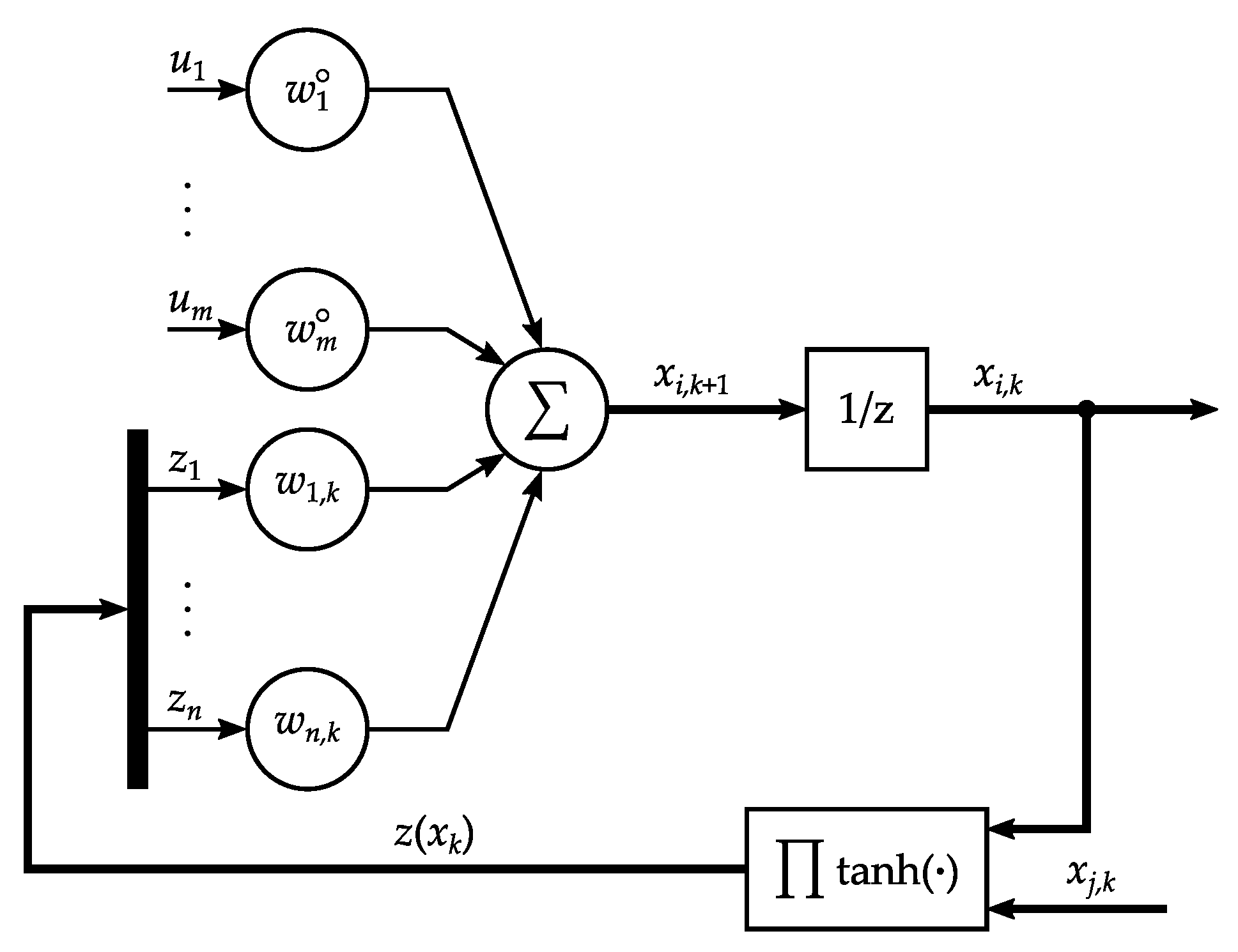
In this paper, we consider the use of a discrete–time RHONN (Figure 3) of the form

$$x_{i,k+1}=w_{i,k}^T{z}_i\left(x_k\right)+w_i^{\circ T}{u}_k,i=1,2,...,n$$

(9)

with

$$z_i\left(x_k\right)=\left(\begin{array}{c}{z}_{i,1}\\ z_{i,2}\\ ⋮\\ z_{i,{\ell }_i}\end{array}\right)=\left(\begin{array}{c}{\displaystyle \prod _{j\in I_1}}{\gamma }_{i_j,k}^{d_{i_j}\left(1\right)}\\ {\displaystyle \prod _{j\in I_2}}{\gamma }_{i_j,k}^{d_{i_j}\left(2\right)}\\ ⋮\\ {\displaystyle \prod _{j\in I_{{\ell }_i}}}{\gamma }_{i_j,k}^{d_{i_j}\left({\ell }_i\right)}\end{array}\right)$$

(10)

for $i=1,2,...,n$, where $\{I_1,I_2,\cdots ,I_{{\ell }_i}\}$ is a collection of ${\ell }_i$ non–ordered subsets of $\{1,2,\cdots ,n+m\}$ and $d_{i_j}\left(1\right),\cdots ,d_{i_j}\left({\ell }_i\right)$ are non–negative integers. $w_i^{\circ T}$ is a constant synaptic weight vector and the functions ${\gamma }_{i,k}$ are in the particular form

$${\gamma }_{i,k}=\left(\begin{array}{c}{\gamma }_{i,1,k}\\ ⋮\\ {\gamma }_{i,n,k}\end{array}\right)=\left(\begin{array}{c}s(x_{1,k})\\ ⋮\\ s\left(x_{n,k}\right)\end{array}\right)$$

where ${\gamma }_{i,j,k}$ are either external inputs or states of neurons passed through a sigmoid function. The functions $s\left(x_{i,k}\right)$, $i=1,\cdots ,n$ are typically sigmoidal monotone–increasing and differentiable functions, called activation functions, having the form

$$s\left(x_{i,k}\right)=\frac{{\alpha }_i}{1+e^{-{\beta }_i{x}_{i,k}}}-{\rho }_i,i=1,\cdots ,n$$

where ${\alpha }_i,{\beta }_i,{\rho }_i>0$ are constants. Sigmoid activation functions can be obtained for ${\alpha }_i={\beta }_i=1$ and ${\rho }_i=0$. In particular, hyperbolic tangent functions are used for ${\alpha }_i={\beta }_i=2$, ${\rho }_i=1$. This last choice simplifies the calculation of the control signal needed to guarantee the closed–loop performance.

Let us now denote, by $w_i^{*}$, $w_i^{\circ *}$, $i=1,\cdots ,n$, the constant (unknown) weights minimizing, on a fixed compact set, the norm of the identification error between (9) and the system to be identified [14]. Therefore, considering the approximation errors

$${ϵ}_{i,k}={\left(w_{i,k}-w_i^{*}\right)}^T{z}_i\left(x_k\right)+{\left(w_i^{\circ }-w_i^{\circ *}\right)}^T{u}_k,$$

for $i=1,\cdots ,n$, one rewrites (9) as

$$x_{i,k+1}=w_i^{*T}{z}_i\left(x_k\right)+w_i^{\circ *T}{u}_k+{ϵ}_{i,k},i=1,\cdots ,n.$$

(11)

For (11), one can consider a RHONN identifier

$${\widehat{x}}_{i,k+1}={\widehat{w}}_{i,k}^T{z}_i\left({\widehat{x}}_k\right)+w_i^{\circ *T}{u}_k,i=1,2,\cdots ,n.$$

(12)

where ${\widehat{x}}_k$ is the estimate of $x_k$ and ${\widehat{w}}_{i,k}$ is the estimate of $w_i^{*}$. Furthermore, in (12), it is assumed that the value of $w_i^{\circ *}$ can be estimated offline. This can be conducted for a large class of systems in affine form since $w_{i,k}^{\circ }$ is constant. The RHONN weight estimation error is

$${\tilde{w}}_{i,k}=w_i^{*}-{\widehat{w}}_{i,k},i=1,\cdots ,n,\forall k\in \mathbb{N}$$

(13)

and its dynamics are

$${\tilde{w}}_{i,k+1}-{\tilde{w}}_{i,k}={\widehat{w}}_{i,k}-{\widehat{w}}_{i,k+1},i=1,\cdots ,n,\forall k\in \mathbb{N}$$

(14)

since $w_i^{*}$ is constant.

The synaptic weights ${\widehat{w}}_{i,k}$ in (12) are online adapted by an extended Kalman filter (EKF) [13,14,15]. The main objective of the EKF is to find the optimal values for the weight vector ${\widehat{w}}_{i,k}^T$, such that the identification errors

$$e_{i,k}=x_{i,k}-{\widehat{x}}_{i,k},i=1,\cdots ,n$$

(15)

are minimized. The EKF solution to the training problem is [23,24]

$${\widehat{w}}_{i,k+1}={\widehat{w}}_{i,k}+{\eta }_{i,k}{K}_{i,k}{e}_{i,k}i=1,\cdots ,n$$

(16)

where

$$K_{i,k}=P_{i,k}{H}_{i,k}{M}_{i,k}\in {\mathbb{R}}^{{\ell }_i}$$

(17)

is the Kalman gain matrix, $i=1,\cdots ,n$ and ${\eta }_{i,k}\in [0,1]$ is the selected learning rate, such that

$${\eta }_{i,k}<\frac{1}{\parallel K_{i,k}\parallel },\forall k\in \mathbb{N},i=1,\cdots ,n.$$

(18)

Here, $P_{i,k}\in {\mathbb{R}}^{{\ell }_i\times {\ell }_i}$ is the predictive error associated covariance matrix defined as

$$P_{i,k+1}=P_{i,k}-K_{i,k}{H}_{i,k}^T{P}_{i,k}+Q_{i,k}$$

(19)

for $i=1,\cdots ,n$, where $Q_{i,k}\in {\mathbb{R}}^{{\ell }_i\times {\ell }_i}$ is the state noise-associated covariance matrix. Moreover, the global scaling matrix $M_{i,k}$ is given by

$$M_{i,k}={\left(R_{i,k}+H_{i,k}^T{P}_{i,k}{H}_{i,k}\right)}^{-1}$$

(20)

for $i=1,\cdots ,n$, where $R_{i,k}\in \mathbb{R}$ and $H_{i,k}\in {\mathbb{R}}^{{\ell }_i}$ is a matrix for which each entry

$$h_{i,j,k}={\left(\frac{\partial {\widehat{x}}_{i,k}}{\partial {\widehat{w}}_{i,j,k}}\right)}_{{\widehat{w}}_{i,k}={\widehat{w}}_{i,k+1}}, \begin{array}{l}i=1,\cdots ,n,\\ j=1,\cdots ,\ell ,\end{array}$$

(21)

is the derivative of one of the neural network output ${\widehat{x}}_{i,k}$ with respect to one neural network weight ${\widehat{w}}_{i,j}$. Note that $H_{i,k}$, $K_{i,k}$ and $P_{i,k}$ are bounded [25]. The dynamics of (13) can be expressed as

$${\tilde{w}}_{i,k+1}={\tilde{w}}_{i,k}-{\eta }_{i,k}{K}_{i,k}{e}_{i,k}$$

(22)

On the other hand, the dynamics of (15) is

$$e_{i,k+1}={\tilde{w}}_{i,k}^T{z}_i\left({\widehat{x}}_k\right)+{ϵ}_{i,k}.$$

(23)

The RHONN identifier presented in this work takes measurements from CarSim^® only for the longitudinal and lateral accelerations $a_{x,k}$ and $a_{y,k}$ and the yaw rate ${\omega }_{z,k}$. Conversely, the identification of the longitudinal and lateral velocities ${\widehat{v}}_{x,k}$ and ${\widehat{v}}_{y,k}$ and roll position and velocity ${\widehat{\alpha }}_{x,k}$ and ${\widehat{\omega }}_{x,k}$ are made using their estimations ${\tilde{v}}_{x,k}$, ${\tilde{v}}_{y,k}$, ${\tilde{\alpha }}_{x,k}$ and ${\tilde{\omega }}_{x,k}$, given by the observer in (5). The proposed neural model is the following:

$$\begin{array}{l}{\widehat{v}}_{x,k+1}={\widehat{w}}_{11}tanh\left({\widehat{v}}_{x,k}\right)+{\widehat{w}}_{12}tanh\left(a_{x,k}\right)\\ {\widehat{v}}_{y,k+1}={\widehat{w}}_{21}tanh\left({\widehat{v}}_{x,k}\right)tanh\left({\widehat{\omega }}_{z,k}\right)+{\widehat{w}}_{22}tanh\left(a_{y,k}\right)\\ \hspace{1em}\hspace{1em}\hspace{1em}+{\widehat{w}}_{23}tanh\left({\alpha }_{x,k}\right)+{\widehat{w}}_{24}tanh\left({\omega }_{x,k}\right)+w_{25}^{\circ }{\delta }_{c,k}\\ {\widehat{\omega }}_{z,k+1}={\widehat{w}}_{31}tanh\left({\delta }_{d,k}\right)+{\widehat{w}}_{32}tanh\left(a_{y,k}\right)+{\widehat{w}}_{33}tanh\left(a_{x,k}\right)\\ \hspace{1em}\hspace{1em}\hspace{1em}+{\widehat{w}}_{34}tanh\left({\widehat{\beta }}_k\right)+{\widehat{w}}_{35}tanh\left({\widehat{\omega }}_{x,k}\right)+w_{36}^{\circ }{M}_{z,k}\\ {\widehat{\alpha }}_{x,k+1}={\widehat{w}}_{41}tanh\left({\widehat{\alpha }}_{x,k}\right)\\ {\widehat{\omega }}_{x,k+1}={\widehat{w}}_{51}tanh\left({\widehat{\alpha }}_{x,k}\right)+{\widehat{w}}_{52}tanh\left({\widehat{\omega }}_{x,k}\right)\end{array}$$

(24)

where $w_{25}^{\circ }$ and $w_{36}^{\circ }$ are constants tuned by the designer.

In (24), the AFS and TV inputs ${\delta }_{c,k}$ and $M_{z,k}$ appear. It is worth noting that ${\delta }_{c,k}$ appears linearly in the model and not implicitly in the lateral front force, as in the discrete–time bicycle model (1). Furthermore, the lateral and yaw dynamics are considered as ideally uncoupled.

It is also important to remind that a neural model is not unique. Model (24) has shown good quality and performance in the identification of CarSim^® measurements, including noise and perturbations when tracking the reference signals.

The stability of the identification errors

$$\begin{array}{lll}{\widehat{e}}_{v_{x,k}}={\widehat{v}}_{x,k}-{\tilde{v}}_{x,k};& {\widehat{e}}_{v_{y,k}}={\widehat{v}}_{y,k}-{\tilde{v}}_{y,k};& {\widehat{e}}_{{\omega }_{z,k}}={\widehat{\omega }}_{z,k}-{\omega }_{z,k};\\ {\widehat{e}}_{{\alpha }_{x,k}}={\widehat{\alpha }}_{x,k}-{\tilde{\alpha }}_{x,k};& {\widehat{e}}_{{\omega }_{x,k}}={\widehat{\omega }}_{x,k}-{\tilde{\omega }}_{x,k};& \end{array}$$

(25)

as well as the stability of the synaptic weight errors

$$\begin{array}{lll}{\tilde{w}}_{1,k}=w_{11}^{*}-{\widehat{w}}_{11,k};& {\tilde{w}}_{2,k}=\left(\begin{array}{l}{w}_{21}^{*}-{\widehat{w}}_{21,k}\\ w_{22}^{*}-{\widehat{w}}_{22,k}\\ w_{23}^{*}-{\widehat{w}}_{23,k}\\ w_{24}^{*}-{\widehat{w}}_{24,k}\end{array}\right);& {\tilde{w}}_{3,k}=\left(\begin{array}{l}{w}_{31}^{*}-{\widehat{w}}_{31,k}\\ w_{32}^{*}-{\widehat{w}}_{32,k}\\ w_{33}^{*}-{\widehat{w}}_{33,k}\\ w_{34}^{*}-{\widehat{w}}_{34,k}\\ w_{35}^{*}-{\widehat{w}}_{35,k}\end{array}\right)\\ {\tilde{w}}_{4,k}=w_{41}^{*}-{\widehat{w}}_{41,k};& {\tilde{w}}_{5,k}=\left(\begin{array}{l}{w}_{51}^{*}-{\widehat{w}}_{51,k}\\ w_{52}^{*}-{\widehat{w}}_{52,k}\end{array}\right)& \end{array}$$

(26)

are discussed in the following theorem.

Theorem 2.

The RHONN identifier (24), trained by the EKF algorithm (15)–(17) and (19)–(21) to identify longitudinal and lateral vehicle velocities ${\tilde{v}}_{x,k}$ and ${\tilde{v}}_{y,k}$, as well as roll position and velocity ${\tilde{\alpha }}_{x,k}$ and ${\tilde{\omega }}_{x,k}$, from the reduced order observer (5) and to identify the vehicle yaw rate ${\omega }_{z,k}$ from CarSim^®, ensures the identification errors (25) to be SGUUB and the weight estimation errors (26) to remain bounded if, for a sufficiently small ${ϵ}_{i,k}$, there exists a constant ${\varphi }_{i,k}$ such that

$$0<{\varphi }_{i,k}<\sqrt{\frac{1-{\eta }_i^2{\parallel K_{i,k}\parallel }^2-{\eta }_i^2}{2(1+{\eta }_i^2)}}$$

where the learning rate factor ${\eta }_i$ is selected satisfying

$$\begin{array}{c}0<{\eta }_i^2<\frac{1}{\parallel K_{i,k}{\parallel }^2+1}\forall i=1,\cdots ,5.\\ \diamond \end{array}$$

Proof of Theorem 2 is given in Appendix B.

2.6. The Inverse Optimal Control for Reference Tracking

The input control laws used for tracking safe references $v_{y,k,\mathrm{ref}}$ and ${\omega }_{z,k,\mathrm{ref}}$ are the active front steering ${\delta }_{c,k}$ (AFS) and the torque vectoring $M_{z,k}$ (TV). No control strategy is presented for the longitudinal velocity $v_{x,k}$, this being a bounded signal, as explained in [11,12].

Based on the structure given in [14,15], the inverse optimal control laws are expressed in matrix form

$$u_k^{*}=\left(\begin{array}{c}{\delta }_{c,k}\\ M_{z,k}\end{array}\right)=-\frac{1}{2}{(R+P_2)}^{-1}{P}_{1,k}$$

(27)

where

$${\displaystyle \phantom{(}{P}_{1,k}=g^{T}P(f\left({\widehat{x}}_k\right)-x_{k+1,\mathrm{ref}}),P_2=\frac{1}{2}{g}^{T}Pg}$$

(28)

and:

$${\widehat{x}}_{k+1}=\left(\begin{array}{c}{\widehat{v}}_{x,k+1}\\ {\widehat{v}}_{y,k+1}\\ {\widehat{\omega }}_{z,k+1}\\ {\widehat{\alpha }}_{x,k+1}\\ {\widehat{\omega }}_{x,k+1}\end{array}\right), {\widehat{x}}_k=\left(\begin{array}{c}{\widehat{v}}_{x,k}\\ {\widehat{v}}_{y,k}\\ {\widehat{\omega }}_{z,k}\\ {\widehat{\alpha }}_{x,k}\\ {\widehat{\omega }}_{x,k}\end{array}\right), x_{k+1,\mathrm{ref}}=\left(\begin{array}{c}{v}_{y,k+1,\mathrm{ref}}\\ {\omega }_{z,k+1,\mathrm{ref}}\end{array}\right), x_{k,\mathrm{ref}}=\left(\begin{array}{c}{v}_{y,k,\mathrm{ref}}\\ {\omega }_{z,k,\mathrm{ref}}\end{array}\right)$$

(29)

$$f\left({\widehat{x}}_k\right)=\left(\begin{array}{c}{\widehat{w}}_{21}tanh\left({\widehat{v}}_{x,k}\right)tanh\left({\widehat{\omega }}_{z,k}\right)+{\widehat{w}}_{22}tanh\left(a_{y,k}\right)\\ +{\widehat{w}}_{23}tanh\left({\widehat{\alpha }}_{x,k}\right)+{\widehat{w}}_{24}tanh\left({\widehat{\omega }}_{x,k}\right)\\ {\widehat{w}}_{31}tanh\left({\delta }_{d,k}\right)+{\widehat{w}}_{32}tanh\left(a_{y,k}\right)+{\widehat{w}}_{33}tanh\left(a_{x,k}\right)\\ +{\widehat{w}}_{34}tanh\left({\widehat{\beta }}_k\right)+{\widehat{w}}_{35}tanh\left({\widehat{\omega }}_{x,k}\right)\end{array}\right)$$

(30)

$$R=\left(\begin{array}{cc}{r}_{11}& 0\\ 0& r_{22}\end{array}\right), P=\left(\begin{array}{cc}{p}_{11}& p_{12}\\ p_{21}& p_{22}\end{array}\right), g=\left(\begin{array}{cc}{w}_{25}^{°}& 0\\ 0& w_{36}^{°}\end{array}\right).$$

(31)

Notice that, from [14,15], it is here considered that $g\left({\widehat{x}}_k\right)=g$ constant, ensuring controllability of the system.

Now, along the same lines of theorem (4.7) of [15], we can state the following theorem.

Theorem 3.

Let $x_{k,\mathrm{ref}}$ be a bounded reference with bounded increments $x_{k+1,\mathrm{ref}}$. If there exists a matrix $P=P^T>0$ such that

$$\begin{gathered} {\displaystyle \phantom{(}\frac{1}{2}{P}_{3,k}+\frac{1}{2}{x}_{k+1,\mathrm{ref}}^{T}P{x}_{k+1,\mathrm{ref}}-\frac{1}{2}{\widehat{x}}_k^{T}P{\widehat{x}}_k-\frac{1}{2}{x}_{k,\mathrm{ref}}^{T}P{x}_{k,\mathrm{ref}}-\frac{1}{4}{P}_{1,k}^T{(R+P_2)}^{-1}{P}_{1,k} \\ \le -\frac{1}{2}\left|\right|P\left|\right|\left|\right|f\left({\widehat{x}}_k\right){\left|\right|}^2-\frac{1}{2}\left|\right|P\left|\right|\left|\right|x_{k+1,\mathrm{ref}}{\left|\right|}^2-\frac{1}{2}\left|\right|P\left|\right|\left|\right|{\widehat{x}}_k{\left|\right|}^2-\frac{1}{2}\left|\right|P\left|\right|\left|\right|x_{k,\mathrm{ref}}{\left|\right|}^2} \end{gathered}$$

(32)

  where

$${\displaystyle \phantom{(}{P}_{1,k}=g^{T}P\left(f\left({\widehat{x}}_k\right)-x_{k+1,\mathrm{ref}}\right);P_2=\frac{1}{2}{g}^{T}Pg;P_{3,k}=f^T\left({\widehat{x}}_k\right)Pf\left({\widehat{x}}_k\right);}$$

(33)

then the control law (27), based on the neural identifier (24), ensures global asymptotic convergence to zero of the tracking errors $e_{v_{y,k}}={\widehat{v}}_{y,k}-v_{y,k,\mathrm{ref}}$ and $e_{{\omega }_{z,k}}={\widehat{\omega }}_{z,k}-{\omega }_{z,k,\mathrm{ref}}$. Moreover, this control law is inverse optimal, i.e., it minimizes the cost functional $\mathcal{J}\left({\xi }_k\right)=V\left({\xi }_k\right)$, with $l\left({\xi }_k\right)=-V^{*}\left({\xi }_{k+1}\right)+V^{*}\left({\xi }_k\right)-u_k^{*T}R{u}_k^{*}$. ⋄

Furthermore, to obtain better performances in terms of tracking errors $e_{v_{y,k}}$ and $e_{{\omega }_{z,k}}$, the authors utilized an offline nature–inspired optimization process known as particle swarm optimization (PSO) for the P matrix determination in Theorem 3 [26,27].

2.7. TV Conversion

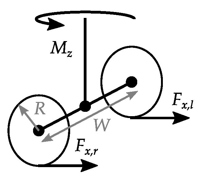
In the following, the yaw moment conversion into electric motor torques is discussed. It is worth mentioning that this strategy does not constitute the originality of this paper. Hence, a simple, intuitive transformation is considered.

The inverse optimal controller (28) provides the amount of yaw moment $M_{z,k}$ needed to maintain the vehicle in safety at any time. Then, $M_{z,k}$ is converted into electric motor torque under the following assumptions.

Assumption 2.

Front and rear wheels on the same side move with equal electric motor torque supposed to be symmetric on left and right, i.e., ${\tau }_{l,c,k}=-{\tau }_{r,c,k}$.

Making use of Assumption 2, it is possible to consider the successive transformation (see Figure 4)

$$M_{z,k}={\displaystyle \frac{W}{2}}(F_{x,r}-F_{x,l}),{\tau }_{l,c,k}=-{\displaystyle \frac{R}{W}}{M}_{z,k},{\tau }_{r,c,k}={\displaystyle \frac{R}{W}}{M}_{z,k}$$

(34)

obtained considering ${\tau }_{i,c,k}=R{F}_{x,i}$, for $i=r,l$.

The electric motor torques to be given for the maneuver execution are determined as in [6,28,29,30].

$${\displaystyle \phantom{(}{\tau }_{i,k}-{\tau }_{L,i,k}-{\alpha }_{i,k}{f}_m=J{\dot{\alpha }}_{i,k}i=r,l,}$$

(35)

where ${\tau }_{L,i,k}$ is the external resistance moment, J is the motor total inertia, $f_m$ is the viscous friction coefficient and ${\alpha }_{i,k}$ is the wheel angular velocity defined as follows:

$${\displaystyle \phantom{(}{\alpha }_{l,k}={\displaystyle \frac{v_{x,k}-{\omega }_{z,k}(\frac{W}{2}+l_r{\beta }_k)}{R}},{\alpha }_{r,k}={\displaystyle \frac{v_{x,k}+{\omega }_{z,k}(\frac{W}{2}-l_r{\beta }_k)}{R}}}$$

(36)

2.8. In–Wheel Electric Machines

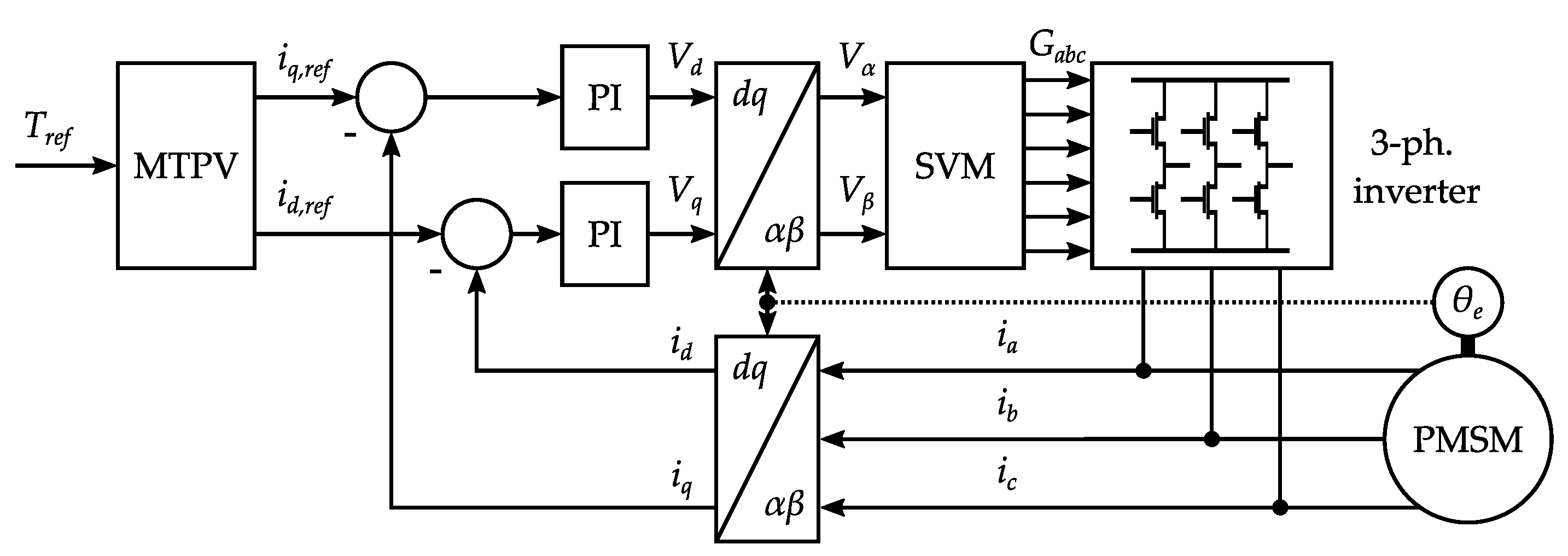
The present study exploits an all–wheel drive constituted by four in–wheel motors. As a reference, outrunner permanent magnet synchronous motors (PMSMs) from the Elaphe M700 series were taken into account [31]. The electrical parameters are listed in

Table 1. In–wheel motor electrical parameters.

Description	Symbol	Value	Unit
Number of pole pairs	p	28	–
PM flux linkage	${\lambda }_p$	17.7	$\mathrm{mWb}$
Phase resistance	R	10	$\mathrm{m\Omega }$
Direct–axis inductance	$L_d$	17	$\mathsf{\mu }\mathrm{H}$
Quadrature–axis inductance	$L_q$	17	$\mathsf{\mu }\mathrm{H}$

.

In particular, field–oriented current control is assumed. For this purpose, the electric machine equations can be written in the rotor reference frame.

$$\begin{gathered} {\displaystyle \phantom{(}{V}_d=L_d\frac{\mathrm{d}{i}_d}{\mathrm{d}t}-p{L}_q\omega i_q+R{i}_d \\ {V}_q=L_q\frac{\mathrm{d}{i}_q}{\mathrm{d}t}+p{L}_d\omega i_d+p{\lambda }_p\omega +R{i}_q} \end{gathered}$$

(37)

where subscripts d (direct) and q (quadrature) denote the rotor axes and label voltages ($V_{d,q}$), currents ($i_{d,q}$) and inductances ($L_{d,q}$). Furthermore, p is the number of pole pairs, R is the phase resistance, ${\lambda }_p$ is the flux linkage of the rotor permanent magnets (PMs) and ω is the rotor angular speed. Equation set (37) describes the dynamic behavior of direct and quadrature currents in the machine. These can be related to the electromagnetic torque, which is the variable of interest in a traction application.

$$T=\frac{3}{2}p{i}_q\left[{\lambda }_p+\left(L_d-L_q\right)i_d\right]$$

(38)

This equation contains a contribution due to PM alignment (left) and a reluctance term (right). Note that, as in this case, when the rotor is perfectly isotropic, $L_d=L_q$ and the torque is given only by PM alignment. To attain traction control, the reference quadrature current is calculated from the desired torque as

$$i_{q,ref}=\frac{2}{3p{\lambda }_p}{T}_{ref}$$

(39)

whereas the direct axis current is set to $i_{d,ref}=0$. However, when angular speed escalates and the back electromotive force of the machine exceeds the source voltage capability, negative direct–axis current is injected, while quadrature current is reduced to extend the speed range of the machine, at the cost of reducing its torque. This operation is known as field weakening and, in this case, is accomplished by means of a maximum torque per volt (MTPV) strategy [32]. Current references are set to separate current proportional–integral (PI) controllers for each rotor axis, as depicted in Figure 5. Then, rotor–frame variables are converted to stator–frame ones and vice versa through phase transformations, which require the electrical angle of the rotor ${\theta }_e$. These conversions aim at establishing the phase voltages in the stator frame and then deciding the switching strategy for the inverter transistors. In this case, a space vector modulation (SVM) switching strategy is assumed. For feedback purposes, a transformation is also required to determine the values of the currents in the rotor frame. Due to causality, the four motors impose a traction torque, while rotor speed is attained as a consequence of vehicle dynamics.

3. Simulation Results

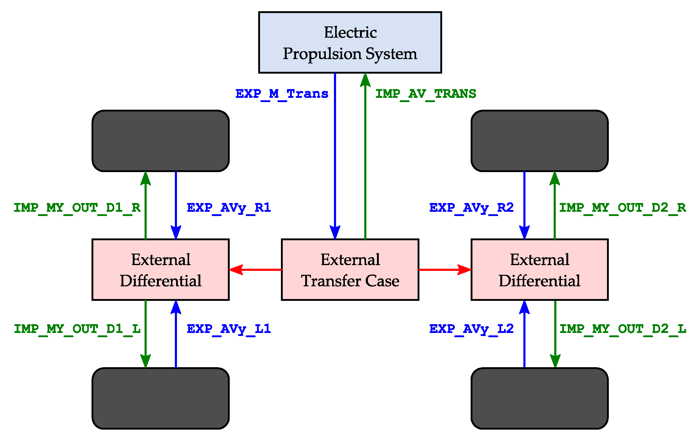
To better test the control quality and performances, the authors made use of the CarSim^® extended model simulator. This tool is able to very closely reproduce the behavior of ground vehicle dynamics. The latest versions of this software allow users to utilize electric powertrains, as well as in–wheel electric motor configurations. For this specific case, several modifications to the CarSim^® basic dataset were needed. As shown in Figure 6, IMP_MY_OUT_Di_j    (i=1,2 and j=L,R) are the signals to be imported. The use of an in–wheel powertrain implies a direct equivalence between the speeds of the electric motor and the vehicle wheel (${\omega }_k={\alpha }_k$). While the vehicle model ran in CarSim^®, the control strategy was executed in Simulink^®in co–simulation.

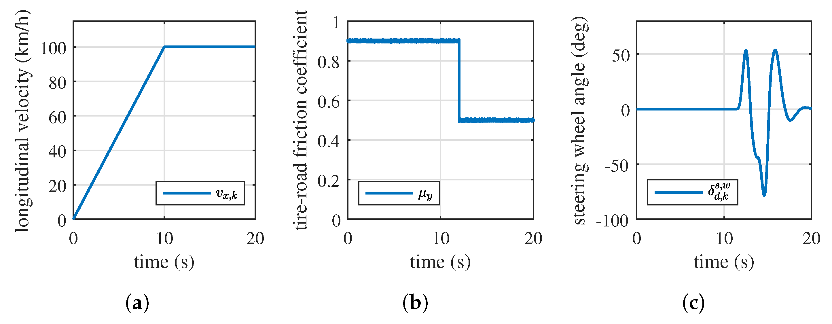
Performance of the proposed nonlinear inverse optimal controller was tested in the interesting case in which the vehicle performed a double–lane change (DLC) maneuver. The DLC maneuver is described in the standard ISO 3888. It represents a vehicle moving with an initial speed set to 27.8 m/s (about 100 km/h), with a released throttle pedal and without braking. To reach the required longitudinal speed given by the DLC standard, the vehicle accelerates uniformly from standstill to 100 km/h in 10 s, as shown in Figure 7a.

A further challenge was taken into account by considering an abrupt change of the tire–road friction coefficient from ${\mu }_{y,k}=0.9$ to ${\mu }_{y,k}=0.5$. These values correspond to dry and wet surfaces, respectively, as represented in Figure 7b. In addition, Figure 7c shows the driver steering angle.

The driver steering wheel angle ${\delta }_{d,k}^{s,w}$ and the steering angle ${\delta }_{d,k}$ are related by a steering ratio of 16:1.

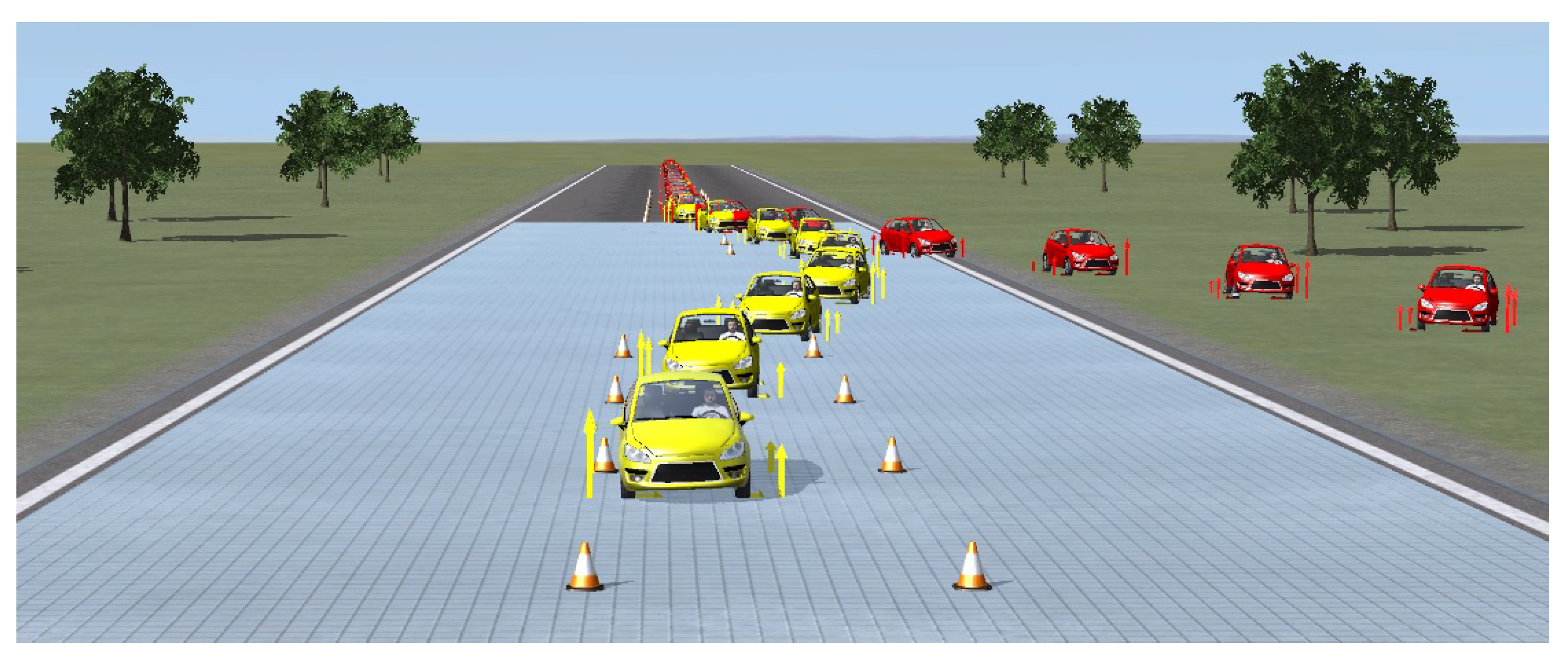
Figure 8 illustrates, with the red vehicle, the behavior when the controller is disabled (open–loop system). The yellow vehicle denotes the case when the controller is enabled (closed–loop system). Note that the controlled vehicle progresses on a safer driving condition, contrary to the uncontrolled vehicle, which shows evident drifting due to adhesion loss.

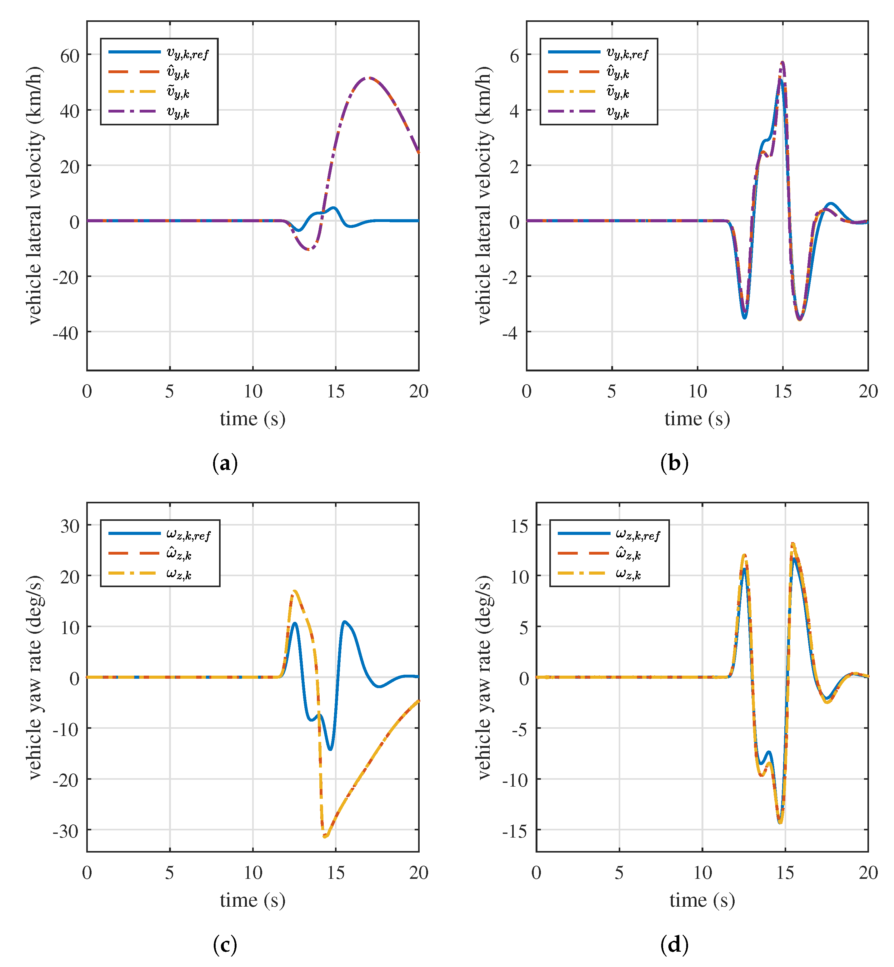
The obtained results are summarized in Figure 9. Specifically, the behavior of the open–loop system is described in Figure 9a,c for the vehicle lateral velocity $v_{y,k}$ and yaw rate ${\omega }_{z,k}$, respectively. On the other hand, Figure 9b,d present the tracking of safe references. Note the favorable shape of the reference tracking, even in presence of unmodeled dynamics when using the CarSim^® full vehicle model.

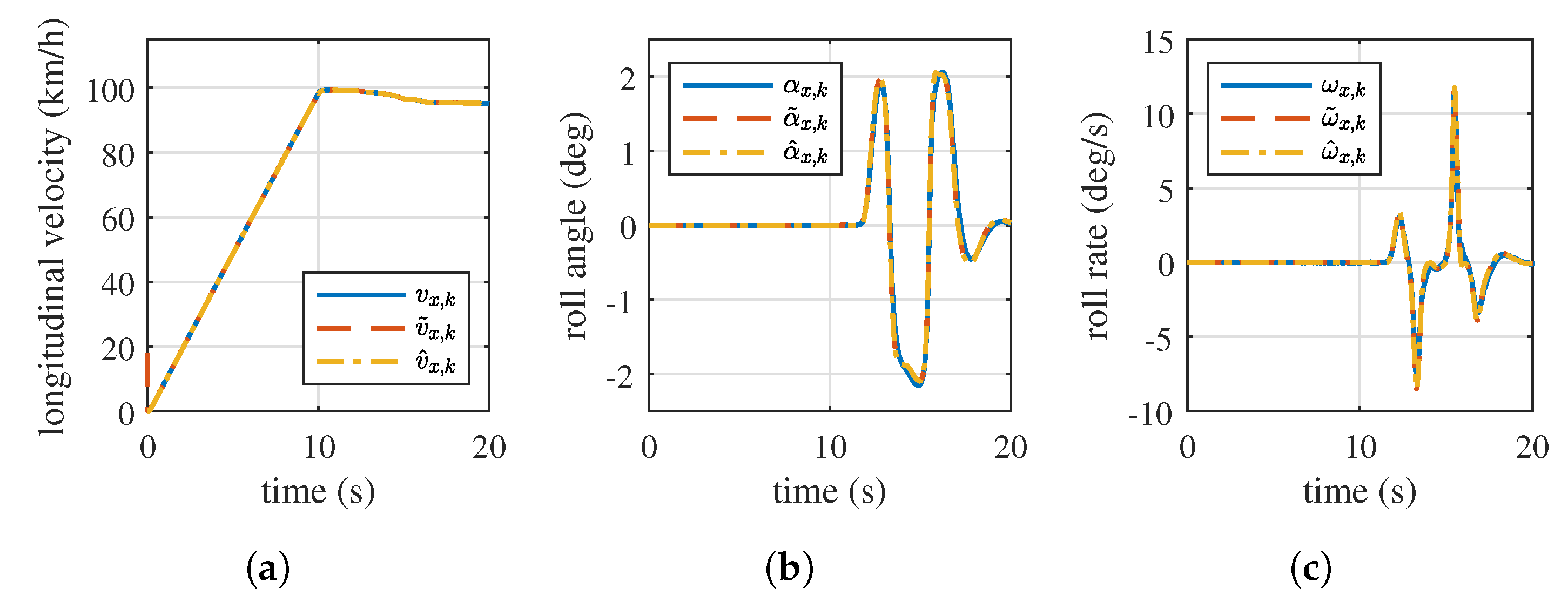
Non–negligible vehicle dynamics were estimated by the discrete–time state observer (5) and then utilized by the neural identifier (24) to provide the neural model for control purposes. Quality and performance of both the observer and the identifier can be observed in Figure 9 in terms of vehicle lateral and yaw dynamics, whereas the longitudinal velocity, roll angle and roll rate are presented in Figure 10a–c, respectively.

The robustness of the observer was tested by applying different initial conditions of the nominal parameters, such as the initial longitudinal velocity, $v_{x,k=0}=0$ and ${\widehat{v}}_{x,k=0}=18$ km/h. Strong and fast convergence was obtained in one time step, as shown in Figure 10a.

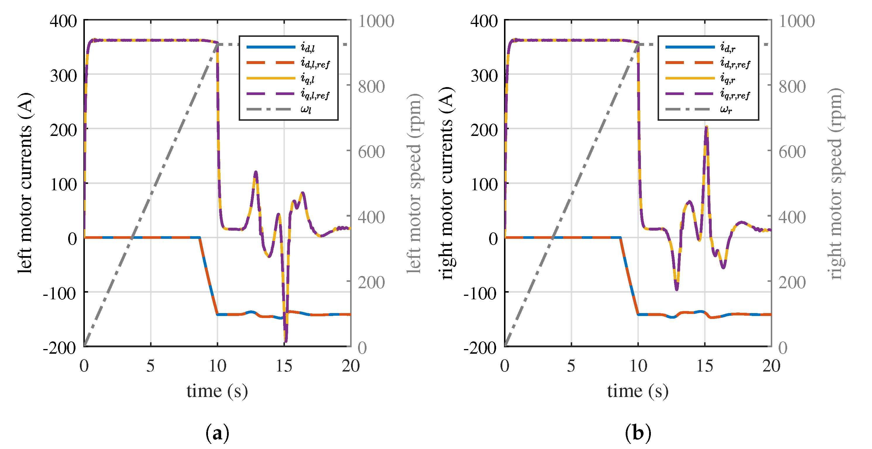
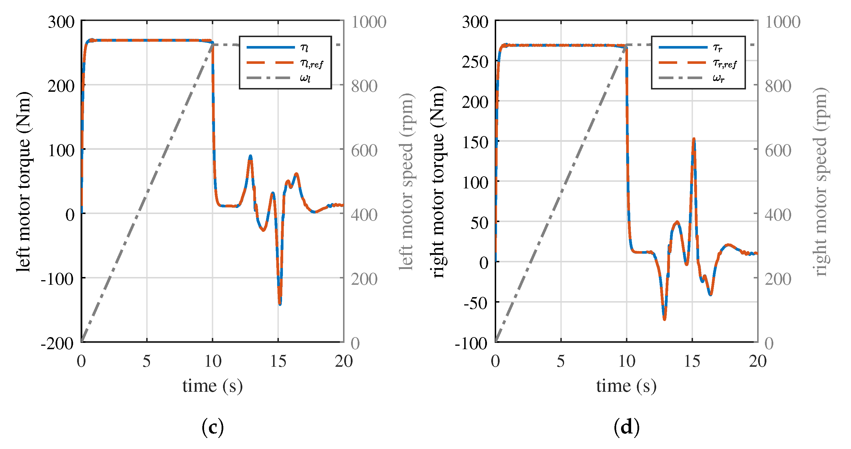
To assess the capability of the powertrain, the in–wheel machines were tested while controlled with the strategy described in Section 2.8. Torque and current time histories—both reference and measured signals—are compared against speed profiles in Figure 11. In particular, a specific torque profile was given for left and right machines, while a speed ramp was imposed on their rotors (rate, $93\mathrm{rpm}/\mathrm{s}$; maximum value, $930\mathrm{rpm}$). The torque profiles held a maximum value around $270\mathrm{Nm}$ as speed escalated. Then, they followed a profile with high dynamic content, while the speed remained constant at its maximum value. The current control demonstrated to provide sufficient bandwidth, as it followed the given reference profiles. Another important aspect is field weakening action at high speed. This was particularly noticeable between 8 and $10\mathrm{s}$, where the current reference generator started injecting a component in the negative direct axis, thus allowing the machine to attain the maximum speed. These results demonstrate the validity of the in–wheel electric machines and their control strategy.

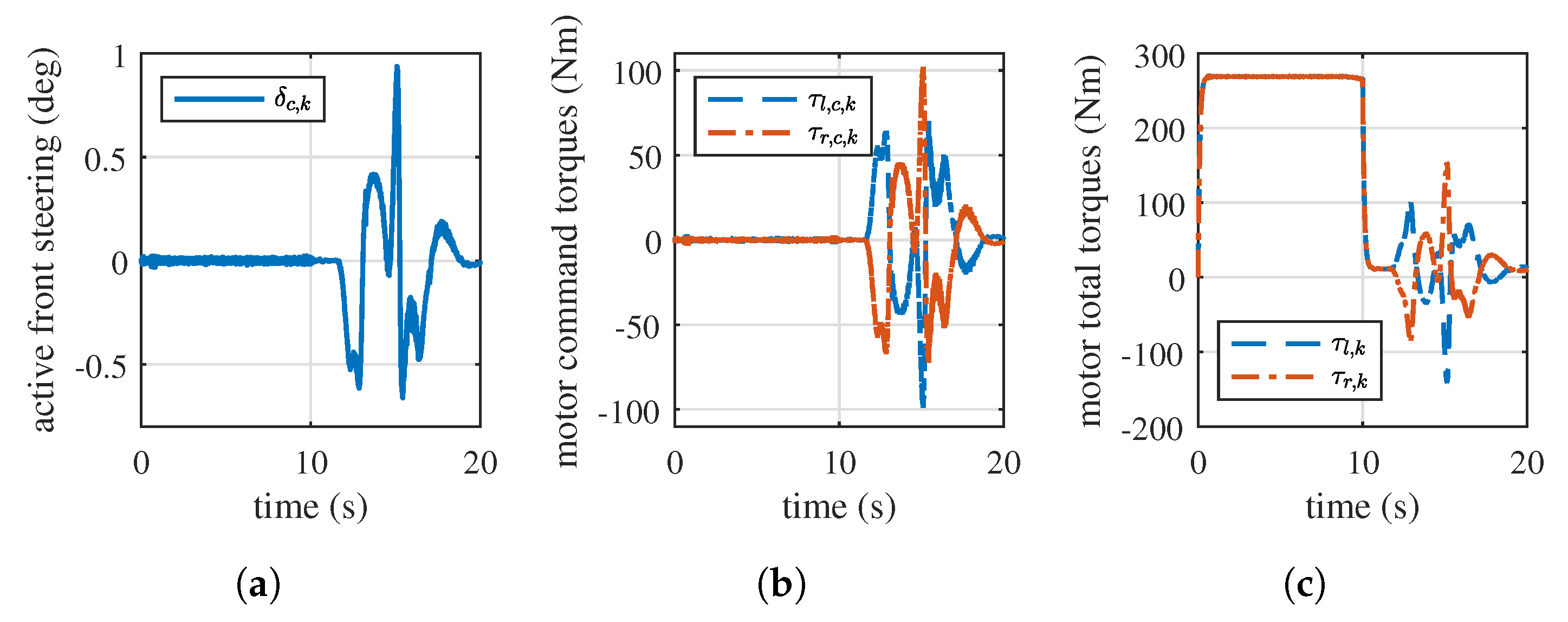
Figure 12 presents the combined control efforts such as active front steering (AFS) and Torque Vectoring (TV). Figure 12a shows the AFS activity, whereas Figure 9b depicts the electric motor torques. The term “command” refers to the fact that these quantities were commanded by the controller. Figure 12c provides a total measure of electric motor torques, the amount needed for the maneuver and the amount needed for stability purposes.

The simulation results show that the control action added to the maneuver did not induce tire instability; in fact, the longitudinal slip angles remained under $8\%$, whereas the lateral slip angles remained under 3 deg, thus ensuring linear behavior of the tire longitudinal and lateral characteristics.

Finally, Figure 13 presents the synaptic neural weights ${\widehat{w}}_{11,k}$, ..., ${\widehat{w}}_{52,k}$ during the online adaptation in the neural identifier (24).

The parameters used in the observer (5), neural identifier (24) and inverse optimal controller (27) are listed in

Table 2. Parameters used in the control scheme.

Symbol	Value	Unit	Symbol	Value	Unit
$D_{y,f,\mathrm{ref}}$	10,500	(N)	${\eta }_i$	0.99	(-)
$C_{y,f,\mathrm{ref}}$	$2.48$	(-)	$P_{i,k=0}$	1	(-)
$B_{y,f,\mathrm{ref}}$	$1.00$	(-)	$w_{26}^{\circ }$	$2797\times {10}^{-3}$	(-)
$D_{y,r,\mathrm{ref}}$	9250	(N)	$w_{36}^{\circ }$	$2497\times {10}^{-2}$	(-)
$C_{y,r,\mathrm{ref}}$	$3.69$	(-)	T	0.001	(s)
$B_{y,r,\mathrm{ref}}$	$2.35$	(-)	$w_{i,k=0}$	1	(-)
${\mu }_{\mathrm{ref}}$	0.9	(-)	$Q_1$	$0.1\times I_2$	(-)
$m_{\mathrm{ref}}=m$	1259	(kg)	$Q_2$	$0.5\times I_4$	(-)
$J_{z,\mathrm{ref}}=J_z$	1343.1	(kg m${}^2$)	$Q_3$	$2\times {10}^{-4}\times I_5$	(-)
${\rho }_0$	$1\times {10}^9$	(-)	$Q_4$	1	(-)
$p_{11}$	$1.6459683\times {10}^{-3}$	(-)	$Q_5$	$I_2$	(-)
$p_{12}$	$82.299$	(-)	$l_f$	1.04	(m)
$p_{22}$	$8.43570\times {10}^5$	(-)	$l_r$	1.56	(m)
R	0.287	(m)	$b_x$	9000	(Ns/m)
h	0.54	(m)	$k_{x,0}$	86,000	(N/m)
W	1.485	(m)	${\tau }_{L,i}$	11.5	(N)
$f_m$	26.6	(Nm/rad)

.

The $P_2$ matrix in Theorem 3, with $P_2>0$ and $P_2=P_2^T$, as well as the constant weights associated to the input control laws $w_{25}^{\circ }$ and $w_{36}^{\circ }$ in (24), were calculated making use of a nature–inspired optimization process PSO. This algorithm, executed offline, is able to find the optimal value of the $P_2$ matrix and the control gains $w_{25}^{\circ }$ and $w_{36}^{\circ }$, depending on the tracking mean square errors, as explained in [26,27].

To verify the advantages of using the proposed control approach, a comparison against other existing strategy was necessary. In this case, the authors propose a fair comparison between optimal and non–optimal methods.

The non–optimal control law utilized for comparison purposes is discussed in [11,12], where a Lyapunov–based control method inverts the lateral tire characteristic, thus yielding the control expressions for AFS and RTV.

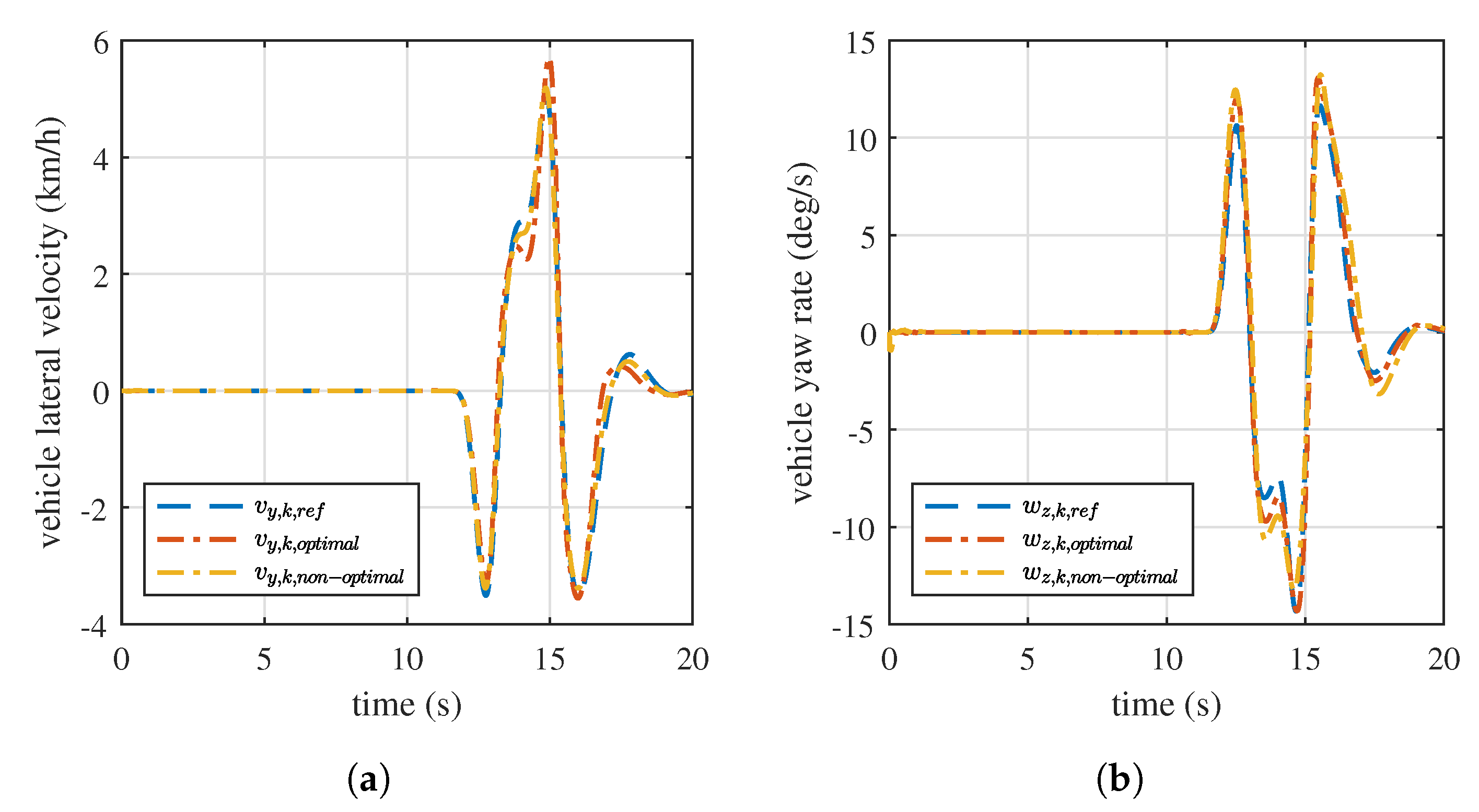
The obtained results are shown in Figure 14. The numerical results, in terms of command activity and root mean square error, are also presented for both optimal and non–optimal control techniques in

Table 3. Comparison between optimal and non–optimal control efforts in terms of command energy spectral density $E(·)$ and root mean square error $RMS(·)$.

Control Technique	$\mathit{E}\left({\mathbf{\delta }}_{\mathit{c},\mathit{k}}\right)$	$\mathit{E}\left({\mathit{M}}_{\mathit{z},\mathit{k}}\right)$	$\mathit{RMS}\left({\mathit{e}}_{{\mathit{v}}_{\mathit{y}}}\right)$	$\mathit{RMS}\left({\mathit{e}}_{{\mathbf{\omega }}_{\mathit{z}}}\right)$
	(deg2s)	(N2m2s)	(km/h)	(deg/s)
Optimal	$0.812$	$2.587\times {10}^5$	$0.293$	$0.617$
Non–optimal	$76.58$	$1.75\times {10}^6$	$0.111$	$1.003$

. Notice that both methods provided a favorable shape in terms of reference tracking errors, as shown in Figure 14. The inverse optimal control approach presented in this work provided better yaw rate tracking, whereas the non–optimal approach led to improved lateral velocity tracking. However, in terms of command activity, the non–optimal method involved significantly larger energy spectral densities of both control actions. Moreover, from a practical standpoint, the non–optimal strategy requires the measurement of the lateral tire forces.

4. Conclusions and Future Works

This paper developed an active controller for the improvement of the stability of electric vehicles equipped with four in–wheel electric motors. The proposed approach offers significant advantages with respect to other conventional methods due to its ability to perform TV without the identification or estimation of the lateral tire forces and the Pacejka’s tire parameters. This contribution represents an important simplification in terms of measured signals when compared to the state of the art.

The control strategy is based on a neural identifier based on RHONN, in which the synaptic weights are trained by an EKF, providing a neural model input–affine. The neural model is then utilized by an inverse optimal controller that ensures asymptotic convergence to the given references. Furthermore, a discrete–time reduced–order state observer is used for the estimation of the lateral velocity and roll position and velocity. This observer ensures exponential stability of the origin of the error system obtained through the Lyapunov theory. Safe references are given for the vehicle lateral velocity and yaw rate based on non–decreasing tire lateral characteristics. Optimal gain settings are ensured by the PSO algorithm, used offline to yield better performances. The mathematical model of the in–wheel electric motor reproduces a realistic behavior of the Elaphe M700 electric machines using field oriented control.

The described approach was tested numerically within a DLC maneuver using a CarSim^® full vehicle model. The obtained results demonstrate enhanced quality and performances of the control action, even in the presence of sudden parametric variation of the tire–road friction coefficient. In addition, the proposed strategy was compared to a non–optimal approach, where improved results in terms of yaw rate tracking and command activity were identified.

Future works should include optimal torque distribution for an all–wheel drive vehicle model, as well as the saturation of the control efforts when reaching full slip.

References

Manca, R.; Circosta, S.; Khan, I.; Feraco, S.; Luciani, S.; Amati, N.; Bonfitto, A.; Galluzzi, R. Performance Assessment of an Electric Power Steering System for Driverless Formula Student Vehicles. Actuators2021, 10, 165. [Google Scholar] [CrossRef]
Farshizadeh, E.; Steinmann, D.; Briese, H.; Henrichfreise, H. A concept for an electrohydraulic brake system with adaptive brake pedal feedback. Proc. Inst. Mech. Eng. Part D J. Automob. Eng.2015, 229, 708–718. [Google Scholar] [CrossRef]
Mazzilli, V.; De Pinto, S.; Pascali, L.; Contrino, M.; Bottiglione, F.; Mantriota, G.; Gruber, P.; Sorniotti, A. Integrated chassis control: Classification, analysis and future trends. Annu. Rev. Control.2021, 51, 172–205. [Google Scholar] [CrossRef]
Ivanov, V.; Savitski, D. Systematization of Integrated Motion Control of Ground Vehicles. IEEE Access2015, 3, 2080–2099. [Google Scholar] [CrossRef]
Zhang, H.; Zhao, W. Decoupling control of steering and driving system for in-wheel-motor-drive electric vehicle. Mech. Syst. Signal Process.2018, 101, 389–404. [Google Scholar] [CrossRef]
Xu, W.; Chen, H.; Zhao, H.; Ren, B. Torque optimization control for electric vehicles with four in-wheel motors equipped with regenerative braking system. Mechatronics2019, 57, 95–108. [Google Scholar] [CrossRef]
Wang, J.; Gao, S.; Wang, K.; Wang, Y.; Wang, Q. Wheel torque distribution optimization of four-wheel independent-drive electric vehicle for energy efficient driving. Control. Eng. Pract.2021, 110, 104779. [Google Scholar] [CrossRef]
Ghosh, J.; Tonoli, A.; Amati, N. Improvement of Lap-Time of a Rear Wheel Drive Electric Racing Vehicle by a Novel Motor Torque Control Strategy; SAE Technical Paper 2017-01-0509; SAE International: Warrendale, PA, USA, 2017. [Google Scholar] [CrossRef]
Ghosh, J.; Tonoli, A.; Amati, N. A Deep Learning Based Virtual Sensor for Vehicle Sideslip Angle Estimation: Experimental Results; SAE Technical Paper 2018-01-1089; SAE International: Warrendale, PA, USA, 2018. [Google Scholar] [CrossRef]
Acosta Lúa, C.; Castillo Toledo, B.; Cespi, R.; Di Gennaro, S. An integrated active nonlinear controller for wheeled vehicles. J. Frankl. Inst.2015, 352, 4890–4910. [Google Scholar] [CrossRef]
Acosta Lúa, C.; Castillo-Toledo, B.; Cespi, R.; Di Gennaro, S. Nonlinear observer-based active control of ground vehicles with non negligible roll dynamics. Int. J. Control. Autom. Syst.2016, 14, 743–752. [Google Scholar]
Rovithakis, G.A.; Christodoulou, M.A. Adaptive Control with Recurrent High–Order Neural Networks; Springer: London, UK, 2000. [Google Scholar]
Sanchez, E.N.; Alanís, A.Y.; Loukianov, A.G. Discrete-Time High Order Neural Control; Springer: Berlin, Germany, 2008. [Google Scholar]
Sanchez, E.N.; Ornelas-Tellez, F. Discrete-Time Inverse Optimal Control for Nonlinear Systems; CRC Press: Boca Raton, FL, USA, 2017. [Google Scholar]
Pacejka, H. Tire and Vehicle Dynamics; Elsevier: Oxford, UK, 2005. [Google Scholar]
Wong, J.Y. Theory of Ground Vehicles; John Wiley & Sons: Hoboken, NJ, USA, 2008. [Google Scholar]
Guiggiani, M. Dinamica del Veicolo; CittàStudi Edizioni: Milan, Italy, 2007. [Google Scholar]
Navarrete Guzmán, A.; Di Gennaro, S.; Rivera Dominguez, J.; Acosta Lúa, C.; Loukianov, A.G.; Castillo-Toledo, B. Enhanced discrete-time modeling via variational integrators and digital controller design for ground vehicles. IEEE Trans. Ind. Electron.2016, 63, 6375–6385. [Google Scholar] [CrossRef]
Luenberger, D. An introduction to observers. IEEE Trans. Autom. Control.1971, 16, 596–602. [Google Scholar] [CrossRef]
Rubio, J.d.J.; Yu, W. Nonlinear system identification with recurrent neural networks and dead-zone Kalman filter algorithm. Neurocomputing2007, 70, 2460–2466. [Google Scholar] [CrossRef]
Haykin, S. Kalman Filtering and Neural Networks; John Wiley & Sons: Hoboken, NJ, USA, 2004; Volume 47. [Google Scholar]
Song, Y.; Grizzle, J.W. The extended Kalman filter as a local asymptotic observer for discrete-time nonlinear systems. J. Math. Syst.1995, 5, 59–78. [Google Scholar]
Eberhart, R.; Kennedy, J. Particle swarm optimization. In Proceedings of the ICNN’95 IEEE International Conference on Neural Networks, Perth, WA, Australia, 27 November–1 December 1995; Volume 4, pp. 1942–1948. [Google Scholar]
Parsopoulos, K.E.; Vrahatis, M.N. Particle Swarm Optimization and Intelligence: Advances and Applications; IGI Global: Hershey, PA, USA, 2010. [Google Scholar]
Folgado, J.; Valtchev, S.S.; Coito, F. Electronic differential for electric vehicle with evenly split torque. In Proceedings of the 2016 IEEE International Power Electronics and Motion Control Conference (PEMC), Varna, Bulgaria, 25–28 September 2016; pp. 1204–1209. [Google Scholar] [CrossRef]
Liu, J.; Zong, C.; Ma, Y. 4WID/4WIS Electric Vehicle Modeling and Simulation of Special Conditions; Technical Paper 2011-01-2158; SAE International: Warrendale, PA, USA, 2011. [Google Scholar] [CrossRef]
Li, Y.; Deng, H.; Xu, X.; Wang, W. Modelling and testing of in-wheel motor drive intelligent electric vehicles based on co-simulation with Carsim/Simulink. IET Intell. Transp. Syst.2019, 13, 115–123. [Google Scholar] [CrossRef]
Soong, W.L.; Miller, T.J.E. Field-weakening performance of brushless synchronous AC motor drives. IEE Proc. Electr. Power Appl.1994, 141, 331–340. [Google Scholar] [CrossRef]
Figure 1.
Control scheme for in–wheel electric vehicles safety stability improvement.
Figure 2.
Bicycle model with roll dynamic.
Figure 3.
RHONN architecture.
Figure 4.
Yaw moment conversion scheme.
Figure 5.
Field–oriented current control strategy.
Figure 6.
CarSim® dataset configuration: four independent torque signals. Involved variables are indicated.
Figure 9.
Open–loop versus closed–loop system comparison in terms of vehicle lateral velocity and yaw rate . (a) Open–loop system. (b) Closed–loop system. (c) Open–loop system. (d) Closed–loop system.
Figure 10.
Observer (5) and neural identifier (24) performances in terms of longitudinal velocity , roll angle and roll rate . (a) Vehicle longitudinal velocity. (b) Vehicle roll angle. (c) Vehicle roll rate.
Figure 11.
Time histories of the current–controlled electric motors. Measured signals (solid) are compared to the references (dashed). (a) Left motor: direct– and quadrature–axis currents. (b) Right motor: direct– and quadrature–axis currents. (c) Left motor: torque and angular speed. (d) Right motor: torque and angular speed.
Figure 12.
Control actions: active front steering , command motor torques , and total motor torques , . (a) Control action: active front steering . (b) Control action: motor command torques. (c) Total in–wheel motor torques.
Figure 13.
Synaptic weights of the neural identifier (24).
Figure 14.
Optimal and non–optimal control strategy comparison. (a) Vehicle lateral velocity tracking. (b) Vehicle yaw rate tracking.