On a Parallelised Diffusion Induced Stochastic Algorithm with Pure Random Search Steps for Global Optimisation

Abstract

We propose a stochastic algorithm for global optimisation of a regular function, possibly unbounded, defined on a bounded set with regular boundary; a function that attains its extremum in the boundary of its domain of definition. The algorithm is determined by a diffusion process that is associated with the function by means of a strictly elliptic operator that ensures an adequate maximum principle. In order to preclude the algorithm to be trapped in a local extremum, we add a pure random search step to the algorithm. We show that an adequate procedure of parallelisation of the algorithm can increase the rate of convergence, thus superseding the main drawback of the addition of the pure random search step.

1. Introduction

If we consider the partition of random type algorithms for global optimisation between those that are adaptive, that is, those that have a search distribution, at a given step, to depend on the distributions of previous steps (see [1,2,3] for comprehensive approaches and, for yet another example, [4]) and those algorithms with steps being independent distributed search variables, it seems that only with those of the second class can we expect to escape the curse of being trapped in local extrema. This curse is surely related to the well known slogan global optimisation requires global information first proposed by Stephens and Baritompa (see [5] and illustrated in [6]). One obvious way to counteract the pernicious effect of adaptivity of the algorithms is to include an intermediate pure random search (PRS) step (see [7]) that will overcame the proclivity of the algorithm to be trapped on a possible local extremum. However, this introduction comes with a price, namely the slowing down of the rate of convergence of the adaptive algorithm. As a countermeasure, we can consider the parallelisation of the algorithm at the pure random stage. Let us briefly state our main objectives in order to give some context to the remainder of this introduction. Our first objective in this work is to study the effect of parallelisation on the rate of convergence of a parallelizable stochastic algorithm for global optimisation with no constraints in the search for the maximum of a function. Our second objective is to study a random adaptive algorithm for global optimisation of functions that may be assumed to attain its extremums at the border of the bounded set where these functions are defined. Thorough and fundamental expositions on the general subject of random algorithms requiring familiarity with probability theory, as well as some knowledge of deterministic and stochastic differential equations and Markov chains, are found in [8,9]. A broad introduction to stochastic algorithms for global optimisation is found in [10]. An excellent reference treaty on stochastic methods for global optimisation is found in [11]; the authors lay a solid ground for further studies, for instance, in detailing extreme value theory and its applications to statistical inference in some stochastic optimisation algorithms. The quest for better performing algorithms for stochastic optimisation continues to develop newer approaches aiming at more general applicability, provable convergence, and stability in regard to small changes in the parameters. An interesting example of such a work is [12], where the objective functions are supposed to be weakly convex, having as a particular case compositions of convex losses with smooth functions seen in machine learning algorithms. Another example may be found in the recent work [13]; the algorithm proposed is akin to the zig-zag algorithm first introduced in [14]—further studied in [15] and with its convergence also studied in [6]—and a thorough comparison of the performance of the introduced algorithm with other well known stochastic optimisation algorithms is detailed. Further results on the convergence of global stochastic optimisation algorithms using perturbed Liapunov function methods are presented in [16]. Let us stress that the subject of stochastic optimisation is broad, encompassing many different types of algorithms such as simulated annealing, genetic algorithms, and tabu search; a review of these different types is provided in [17], detailing advantages and disadvantages and summarising the literature on optimal values of the inputs. There are many instances of the idea that the algorithm may, in itself, guide the search into more promising regions; for instance, in [18], modifications of the pure random search algorithm are proposed following this idea—implemented using the regularity of the function to determine the more promising regions—and we quote, ...We think that if the objective function satisfies some conditions such as continuity, the Lipschitz condition or differentiability etc., the regions containing the minimal points are easy to be determined. If the algorithm generates many points in the regions of this kind, the probability of success will be large.

Fruitful ideas to build global optimisation algorithms with stochastic differential equations were previously published in, for instance, [19,20,21,22,23,24,25,26]. For numerical methods in stochastic differential equations, a fundamental reference is [27]. The splendid book [19] provides a well-founded approach to the convergence of algorithms either using functional compactness arguments or weak convergence results; some of the algorithms studied are taken as perturbations of ideal deterministic algorithms by an additive noise, not necessarily Gaussian, satisfying regularity properties. The idea of defining the intensity of the additive noise, the volatility of the stochastic differential equation by an annealing rate decreasing to zero with increasing time, is proposed in [21], and weak convergence is studied. In [25], the convergence of the studied algorithm for global optimisation with constraints is established for general nonconvex, smooth functions; the stochastic differential equation underpinning the algorithm .has as a drift the symmetric of the gradient of the function—a well known approach for obtaining a solution to an unconstrained optimisation problem considering the ordinary differential equation—and for the volatility, the square root of a positive function denominated annealing schedule with a parameter to be chosen according to the problem under analysis. This approach was already studied in [20], where a detailed justification for the choice of the stochastic differential equation is given, alongside many interesting related results. In [26], the authors use Euler discretisation of a stochastic differential equation with mean reversion, in which the volatility is suitably modified in order to reduce the Gaussian noise contribution as the number of iterations increase; the method is tested against 14 classical functions, and the results indicate that the random search guided by the trajectory of a discretised diffusion perform well. The fine study of stochastic algorithms based on stochastic differential equations can be read in [28], where, using perturbed Liapunov function methods, stability results of the algorithms are established. Furthermore, in [16], an algorithm of simulated annealing-type procedure is studied and the following recommendation is stated: ...whenever possible, one can and should use parallel processors....

In this work, we do not need much of a theoretical background on parallel computing, as we use a standard computation tool to take advantage of the processors being able to compute either with the specification of working independently or not. Some general references for the study of parallel algorithms are [29,30,31]. Early efforts on the parallelisation of those stochastic algorithms that may be called by the random search type can be read in [32], where a particular structure of the algorithm is designed using several units capable of processing data independently, notwithstanding communication with the units during the computation. In [29], a collective work, there is an excellent review of the main ideas of parallelisation techniques for global optimisation algorithms. More recently, in [33], the authors propose a framework to estimate the parallel performance of a given algorithm by analysing the runtime behaviour of its sequential version; the goal is achieved by approximating the runtime distribution of the sequential process with statistical methods, and then the runtime behaviour of the parallel process can be predicted by a model based on order statistics. The method we develop in this work bears some resemblance with this general idea.

As we previously observed, some fundamental random search algorithms for global optimisation built using discretised stochastic differential equations have as volatilities—that is, variances—parametrised quantities derived from simulated annealing principles. Parallelisation of simulated annealing type algorithms were studied by several authors. A precursor work is [34], where the simulated annealing algorithm is mapped onto a dynamically structured tree of processors; the algorithm presented achieves speedups between ${log}_{2}N$ and $(N+{log}_{2}N)/2$, N being the number of processors. Another important work is a volume edited by Robert Azencott, from which [35] is a paradigmatic chapter. In [36], five parallel algorithms for global optimisation are studied; these algorithms are categorised by the amount of information exchanged among the different parallel runs with the asynchronous approach, being such that no information is exchanged among parallel runs. The parallelisation we propose is asynchronous, and the parallel runs are independent. In [37], there are three proposals of parallel algorithms for simulated annealing that fall in a similar categorisation for the the amount of information exchanged among the different parallel runs leading to independent, semi-independent, and co-operating searches. An important reference on the same vein is [38], reporting on five conversions of simulated annealing algorithm from sequential-to-parallel forms on high-performance computers and their application to a set of standard function optimisation problems. In the algorithm proposal of [39], a common feature of simulated annealing algorithms, that is, adaptive cooling based on variance, is abandoned; instead, the algorithm resamples the states across processors periodically, and the resampling interval is tuned according to the success rate for each specific number of processors.

We now present in greater detail the contents and main contributions of this work. The first one is to develop and study a novel formal description of parallelisation of random algorithms for global optimisation with no constraints, and the second one is to introduce and study a novel stochastic differential equation-based algorithm suited to functions attaining the extremum at some points of the border of the domain of definition, for instance, unbounded functions. On the first contribution, in Theorem 1, we detail a proof of the convergence of the pure random search algorithm for measurable functions, using simple results of martingale theory in discrete time, with the main purpose of highlighting the perspective used in this work, to wit, a stochastic algorithm may be seen as a sequence of random variables. With this perspective, in Theorem 2, we show that two convergent pure random search algorithms associated with the same function converge to random variables with the same law. We define, in Definition 3, the rate of convergence of a random algorithm and, in Definition 4, the parallelisation of such an algorithm, following the MPI standard, which is designed for distributed memory with multiple kernels of computation. Theorem 3 is another of the main contributions of this work, since we prove an estimate showing the improvement of the rate of convergence of a parallelised algorithm measured with respect to the nonparallelised version of the algorithm. We show that the parallelisation of the pure random search algorithm behaves in conformity with the results of Theorem 3 with examples of standard test functions for global optimisation. For the second main contribution of this work, in Section 4, we introduce a novel algorithm using stochastic differential equations based on a maximum principle, which is specially suited for unbounded functions; we consider an example that we treat both in the parallelised and nonparallelised versions of the algorithm, thus showing again the advantage of parallelising a random algorithm. The proposed algorithm is different from the algorithms proposed in the literature, in particular, in the works referred above in the paragraph on global optimisation algorithms with stochastic differential equations, and we intend to further explore the properties of this new algorithm in future work. Broadly stated, the main difference stems from the fact that the stochastic differential equation is built in order for the algorithm to be a martingale and for a maximum principle to be applied.

2. On the Parallelisation of Random Algorithms

The introduction of a pure random search step in an adaptive stochastic algorithm for global optimisation is an auxiliary device to avoid missing the global extremum. However, keeping in mind that adaptive algorithms are introduced to increase the convergence rates, the pure random search step is counterproductive, since it slows down the whole algorithm.

Thus, we propose parallelisation of the algorithm at the pure random search step level in order to improve the global rate of convergence of the algorithm. For completeness, we first describe a martingale approach to pure random search. Next, in Section 2.2, we show that, with an appropriate definition of the rate of convergence, parallelisation of a stochastic algorithm improves the global rate of convergence.

2.1. Pure Random Search Revisited

A probabilistic description of the pure random search may be defined as follows.

Definition 1

(Pure random search for global optimisation). A pure random search algorithm for the global maximisation of a function f on a compact set K is a sequence ${\left(f\left(Y_n\right)\right)}_{n\ge 0}$ of random variables, such that:

 (i) 

The function $f:K\subset {\mathbb{R}}^d⟶\mathbb{R}$, defined on K a compact set of ${\mathbb{R}}^d$, is measurable.

 (ii) 

The sequence $X_0,X_1,\cdots X_n,\cdots$ is a sequence of independent and identically distributed (IID) random variables with $X⌢\mathcal{U}\left(K\right)$, that is, X is uniformly distributed in K. We recall that, with λ denoting the Lebesgue measure over ${\mathbb{R}}^d$ we have—with the symbol ⌢ denotingwith probability law—that:

$$X⌢\mathcal{U}\left(K\right)\iff \forall B\in \mathcal{B}\left(K\right),\mathbb{P}\left[B\right]=\frac{1}{\lambda \left(K\right)}{\int }_{B}d\lambda .$$

(1)

 (iii) 

The sequence $Y_0,Y_1,\cdots Y_n,\cdots$ is a sequence of random variables with values in K defined for almost all $\omega \in \mathsf{\Omega }$ by $Y_0=X_0$ and for $n\ge 1$:

$$Y_{n+1}\left(\omega \right)=\left\{\begin{array}{cc}{X}_{n+1}\left(\omega \right)\hfill & iff\left(X_{n+1}\left(\omega \right)\right)>f\left(Y_n\left(\omega \right)\right)\hfill \\ Y_n\left(\omega \right)\hfill & iff\left(X_{n+1}\left(\omega \right)\right)\le f\left(Y_n\left(\omega \right)\right),\hfill \end{array}\right.$$

(2)

with the consequence that ${\left(f\left(Y_n\right)\right)}_{n\ge 0}$ is a nondecreasing sequence for almost all $\omega \in \mathsf{\Omega }$.

Four our purposes, we recall an essential definition.

Definition 2

(The essential supremum of a function over a compact set). The essential supremum ${\alpha }_f$ of the function f over K is given by:

$$\begin{array}{cc}\hfill {\alpha }_f& :=inf\left\{t:\lambda \left(\left\{x\in K:f\left(x\right)>t\right\}\right)=0\right\}=\hfill \\ \hfill & =inf\left\{t:f\left(x\right)\le t,\lambda almost everywhere on K\right\}=\hfill \\ \hfill & =sup\left\{t:\lambda \left(\left\{x\in K:f\left(x\right)>t\right\}\right)>0\right\}.\hfill \end{array}$$

(3)

We next single out Hypothesis 1 with the purpose of focusing on the most interesting cases for our study. In Remark 1, we identify the extension of Theorem 1 to the excluded cases of this hypothesis.

Hypothesis 1.

We will suppose that ${\alpha }_f\in \mathbb{R}$. This hypothesis implies that, for all $p\ge 1$, we have that f is of p-power integrable (see for instance ([40], p. 190)).

We now present the convergence result for the random algorithm of pure random search for global optimisation.

Theorem 1

(On the convergence of the pure random search algorithm). Under Hypothesis 1, we have that, for the pure random search algorithm in Definition 1:

 1. 

The sequence ${\left(f\left(Y_n\right)\right)}_{n\ge 0}$ is asubmartingalewith respect to its natural filtration $\mathbb{F}={\left({\mathcal{F}}_n\right)}_{n\ge 0}$, that is, with: ${\mathcal{F}}_n:=\sigma (f\left(Y_0\right),f\left(Y_1\right),\cdots ,f\left(Y_n\right))$.

 2. 

The sequence ${\left(f\left(Y_n\right)\right)}_{n\ge 0}$ convergesalmost surelyto a random variable ${\mathbb{Y}}_{\infty }^f$ such that, with ${\alpha }_f$ the essential supremum of f over K in Definition 2,

$$\mathbb{P}\left[{\mathbb{Y}}_{\infty }^f\ge {\alpha }_f\right]=1,$$

(4)

that is, the random variable ${\mathbb{Y}}_{\infty }^f$ is astrongsolution of the global optimisation problem of f over K.

Proof. 

We first observe that the random variables of the sequence ${\left(f\left(Y_n\right)\right)}_{n\ge 0}$ are integrable. In fact as we have, by Formula (2) and by the righthand side of Formula (1), that:

$$\begin{array}{cc}\hfill \mathbb{E}\left[|f\left(Y_{n+1}\right)|\right]& =\mathbb{E}\left[|f\left(X_{n+1}\right)1{\mathrm{I}}_{\{f\left(X_{n+1}\right)>f\left(Y_n\right)\}}+f\left(Y_n\right)1{\mathrm{I}}_{\{f\left(X_{n+1}\right)\le f\left(Y_n\right)\}}|\right]\le \hfill \\ \hfill & \le \mathbb{E}\left[|f\left(X_{n+1}\right)|\right]+\mathbb{E}\left[|f\left(Y_n\right)|\right]=\frac{1}{\lambda \left(K\right)}{\int }_K\left|f\left(x\right)\right|d\lambda +\mathbb{E}\left[|f\left(Y_n\right)|\right],\hfill \end{array}$$

(5)

and we may conclude by induction. Now, since the conditional expectations are well defined and the sequence ${\left(f\left(Y_n\right)\right)}_{n\ge 0}$ is a nondecreasing sequence for almost all $\omega \in \mathsf{\Omega }$, we have that:

$$0\le \mathbb{E}\left[f\left(Y_{n+1}\right)-f\left(Y_n\right){\mathcal{F}}_n\right]=\mathbb{E}\left[f\left(Y_{n+1}\right){\mathcal{F}}_n\right]-f\left(Y_n\right),$$

and so we have the first statement in Theorem 1. In order to prove that the submartingale ${\left(f\left(Y_n\right)\right)}_{n\ge 0}$ converges, we will take advantage of Hypothesis 1 to obtain an uniform bound on the terms in the furthest left-hand side of Formula (5). Since we have that:

$${\alpha }_f=inf\left\{t:f\left(x\right)\le t,\lambda \mathrm{a}\mathrm{l}\mathrm{m}\mathrm{o}\mathrm{s}\mathrm{t} \mathrm{e}\mathrm{v}\mathrm{e}\mathrm{r}\mathrm{y}\mathrm{w}\mathrm{h}\mathrm{e}\mathrm{r}\mathrm{e} \mathrm{o}\mathrm{n} K\right\}<+\infty ,$$

we have that, for every $ϵ>0$, there exists $t_{ϵ}$, such that ${\alpha }_f\le t_{ϵ}<{\alpha }_f+ϵ$, and such that $f\left(x\right)\le t_{ϵ}$ almost everywhere on K with respect to $\lambda$. This implies the uniform bound:

$$\underset{n\ge 0}{sup}\mathbb{E}\left[|f\left(Y_n\right)|\right]\le t_{ϵ}<+\infty .$$

(6)

As a consequence of the bound in Formula (6), we have, by a standard result on martingale theory (see ([41], p. 50)), that the submartingale ${\left(f\left(Y_n\right)\right)}_{n\ge 0}$ converges almost surely to a random variable that we denote by ${\mathbb{Y}}_{\infty }^f$. In order to prove that ${\mathbb{Y}}_{\infty }^f$ is a strong solution of the maximisation problem for f over K—defined to be a solution such that Formula (4) is satisfied—we consider, for an arbitrary $ϵ>0$, the fixed set defined by:

$$E_{{\alpha }_f-ϵ}:=\left\{x\in K:f\left(x\right)>{\alpha }_f-ϵ\right\},$$

(7)

and we proceed with the following sequence of observations. Without loss of generality, we may assume, as an Hypothesis 2, that ${\alpha }_f>0$, since, by Hypothesis 1, if it is otherwise, we can always consider a translation of f.

 (j) 

For $ϵ<{\alpha }_f$ we have that:

$$\mathbb{P}\left[\underset{n\to +\infty }{lim\; sup}\left\{X_n\in E_{{\alpha }_f-ϵ}\right\}\right]=1.$$

(8)

We first observe that, by the fact that ${\alpha }_f=sup\left\{t:\lambda \left(\left\{x\in K:f\left(x\right)>t\right\}\right)>0\right\}$, and as a consequence of a standard supremum argument, we have that

$$\begin{array}{cc}\hfill \mathbb{P}\left[X_n\in E_{{\alpha }_f-ϵ}\right]& =\mathbb{P}\left[f\left(x\right)>{\alpha }_f-ϵ\right]\ge \frac{1}{\lambda \left(K\right)}{\int }_{\{f\left(x\right)>{\alpha }_f-ϵ\}}f\left(x\right)d\lambda \left(x\right)\ge \hfill \\ \hfill & \ge ({\alpha }_f-ϵ)\frac{\lambda \left(\{x:f\left(x\right)>{\alpha }_f-ϵ\}\right)}{\lambda \left(K\right)}>0.\hfill \end{array}$$

(9)

Now, since the sequence ${\left(X_n\right)}_{n\ge 0}$ is an IID sequence, by the converse of Borel–Cantelli lemma, as a consequence of Formula (9), ${\sum }_{n=0}^{+\infty }\mathbb{P}\left[X_n\in E_{{\alpha }_f-ϵ}\right]=+\infty$, and so the announced result in Formula (8) follows.

 (jj) 

Almost surely, we will have $Y_n\in E_{{\alpha }_f-ϵ}$ for some integer $n\ge 0$, that is, more precisely,

$$\exists {\mathsf{\Omega }}_0\in \mathcal{F},\mathbb{P}\left[{\mathsf{\Omega }}_0\right]=1,\forall {\omega }_0\in {\mathsf{\Omega }}_0\exists n_0=n_0\left({\omega }_0\right),Y_{n_0}\left({\omega }_0\right)\in E_{{\alpha }_f-ϵ}.$$

Let us suppose the contrary, that is,

$$\forall {\mathsf{\Omega }}_0\in \mathcal{F},\mathbb{P}\left[{\mathsf{\Omega }}_0\right]=1,\exists {\omega }_0\in {\mathsf{\Omega }}_0\forall n,Y_n\left({\omega }_0\right)\notin E_{{\alpha }_f-ϵ}.$$

(10)

Consider, for $ϵ<{\alpha }_f$, the set,

$${\mathsf{\Omega }}_0:=\underset{n\to +\infty }{lim\; sup}\{X_n\in E_{{\alpha }_f-ϵ}\}=\bigcap _{m\ge 0}\bigcup _{n\ge m}\{X_n\in E_{{\alpha }_f-ϵ}\},$$

(11)

which we know, by Formula (8), to have full probability and select ${\omega }_0\in {\mathsf{\Omega }}_0$ according to the condition in Formula (10). Now, by the definition of ${\mathsf{\Omega }}_0$ in Formula (11), there exists $n_0>1$, such that $X_{n_0}\left({\omega }_0\right)\in E_{{\alpha }_f-ϵ}$, that is such that $f\left(X_{n_0}\left({\omega }_0\right)\right)>{\alpha }_f-ϵ$. However, by the condition in Formula (10), we have that $f\left(Y_{n_0-1}\left({\omega }_0\right)\right)\le {\alpha }_f-ϵ$, and so, by the definition of the sequence ${\left(Y_n\right)}_{n\ge 0}$ in Formula (2), we should have that $Y_{n_0}\left({\omega }_0\right)=X_{n_0}\left({\omega }_0\right)$ and so $f\left(Y_{n_0}\left({\omega }_0\right)\right)>{\alpha }_f-ϵ$, that is, $Y_{n_0}\left({\omega }_0\right)\in E_{{\alpha }_f-ϵ}$, a statement that contradicts the condition in Formula (10).

 (jjj) 

We have the final conclusion of the second statement in the theorem, Formula (4), that is:

$$\mathbb{P}\left[{\mathbb{Y}}_{\infty }^f\ge {\alpha }_f\right]=1.$$

Take $ϵ<{\alpha }_f$ and ${\mathsf{\Omega }}_0\in \mathcal{F}$ satisfying Observation (jj), that is, a set of full probability and such that,

$$\forall {\omega }_0\in {\mathsf{\Omega }}_0\exists n_0=n_0\left({\omega }_0\right),Y_{n_0}\left({\omega }_0\right)\in E_{{\alpha }_f-ϵ}.$$

Now, since the sequence ${\left(f\left(Y_n\right)\right)}_{n\ge 0}$ is almost surely nondecreasing, for all ${\omega }_0\in {\mathsf{\Omega }}_0$ and the adequate $n_0=n_0\left({\omega }_0\right)$, we can write:

$$\forall n\ge n_0,f\left(Y_n\left({\omega }_0\right)\right)\ge f\left(Y_{n_0}\left({\omega }_0\right)\right)>{\alpha }_f-ϵ,$$

a condition that implies ${lim}_{n\to +\infty }f\left(Y_n\left({\omega }_0\right)\right)=:{\mathbb{Y}}_{\infty }^f\left({\omega }_0\right)\ge {\alpha }_f-ϵ$. We have thus shown that

$$\forall 0<ϵ<{\alpha }_f,\mathbb{P}\left[{\mathbb{Y}}_{\infty }^f\ge {\alpha }_f-ϵ\right]=1,$$

a condition that, by a standard argument, implies Formula (4).

Being so, the proof of the theorem is now complete.    □

Remark 1

(On the case of an infinite essential supremum). In order to extend Theorem 1 to the case ${\alpha }_f=+\infty$, we may consider that

$$\underset{n\ge 0}{sup}\mathbb{E}\left[f^{+}\left(Y_n\right)\right]<+\infty ,$$

a condition that, for any submartingale, is equivalent to ${sup}_{n\ge 0}\mathbb{E}\left[|f\left(Y_n\right)|\right]<+\infty$, that is, the sequence ${\left(f\left(Y_n\right)\right)}_{n\ge 0}$ is bounded in $L^1$ (see ([41], pp. 50–51)). Furthermore, by observing that, if

$${\alpha }_f=sup\left\{t:\lambda \left(\left\{x\in K:f\left(x\right)>t\right\}\right)>0\right\}=+\infty ,$$

we have for arbitrary $M>0$ that $\lambda \left(\left\{x\in K:f\left(x\right)>M\right\}\right)>0$, and so we can consider, instead of $E_{{\alpha }_f-ϵ}$, the set $E_{{\alpha }_f,M}=\left\{x\in K:f\left(x\right)>M\right\}$. We then show that $\mathbb{P}\left[{\mathbb{Y}}_{\infty }^f\ge M\right]=1$ with a similar proof, a condition that, in turn, implies that ${\mathbb{Y}}_{\infty }^f=+\infty$ almost surely.

We now state a remark and an important result on the laws of the solution of the global optimisation problem by means of pure random search that we will use in the sequel.

Remark 2

(On the laws of the variables of the algorithm). Consider the two sequences $X_0,X_1,\cdots X_n,\cdots$, and $X_0^{\prime },X_1^{\prime },\cdots X_n^{\prime },\cdots$ of IID random variables with $X⌢\mathcal{U}\left(K\right)$, and let $f\left(Y_0\right),f\left(Y_1\right),\cdots f\left(Y_n\right),\cdots$ and $f\left(Y_0^{\prime }\right),f\left(Y_1^{\prime }\right),\cdots f\left(Y_n^{\prime }\right),\cdots$ be the corresponding pure random search algorithms according to Definition 1. Then, for all $n\ge 0$, we have that $f\left(Y_n\right)$ and $f\left(Y_n^{\prime }\right)$ have the same law. In fact, a simple proof by induction shows that, for every $n\ge 0$, the law of $Y_n$—and consequently, the law of $f\left(Y_n\right)$—only depends on the law of $(X_0,X_1,\cdots X_n)$.

Theorem 2

(On the unicity of the global optimisation solution of pure random search). Suppose that ${\alpha }_f$, the essential supremum of f over the compact K, is finite. Let ${\left(f\left(Y_n\right)\right)}_{n\ge 0}$ and ${\left(f\left(Y_n^{\prime }\right)\right)}_{n\ge 0}$ be two pure random search algorithms associated with $X_0,X_1,\cdots X_n,\cdots$ and $X_0^{\prime },X_1^{\prime },\cdots X_n^{\prime },\cdots$, two sequences of IID random variables with $X⌢\mathcal{U}\left(K\right)$, as in Remark 2. Suppose that these random algorithms converge to ${\mathbb{Y}}_{\infty }$ and ${\mathbb{Y}}_{\infty }^{\prime }$, respectively. Then, we have that $\mathbb{P}[{\mathbb{Y}}_{\infty }\ne {\mathbb{Y}}_{\infty }^{\prime }]=0$, and so ${\mathbb{Y}}_{\infty }$ and ${\mathbb{Y}}_{\infty }^{\prime }$ have the same law.

Proof. 

We can consider the sequence defined for $n\ge 0$ by:

$$Z_n:=\left\{\begin{array}{cc}{Y}_n\hfill & \mathrm{i}\mathrm{f} f\left(Y_n\right)\ge f\left(Y_n^{\prime }\right)\hfill \\ Y_n^{\prime }\hfill & \mathrm{i}\mathrm{f} f\left(Y_n\right)<f\left(Y_n^{\prime }\right).\hfill \end{array}\right.$$

(12)

Now, we may observe the following. Firstly, we have that, almost surely for $n\ge 0$, $f\left(Z_n\right)=max(f\left(Y_n\right),f\left(Y_n^{\prime }\right))$ as an immediate consequence of the definition in Formula (12). Then, we have that, almost surely, ${\left(f\left(Z_n\right)\right)}_{n\ge 0}$ is a nondecreasing sequence, as it is defined as the pointwise maximum of two nondecreasing sequences. Lastly, since, for all $n\ge 0$, we have that $Y_n$ and $Y_n^{\prime }$ have the same law (see Remark 2), and since, by Formula (2), we have that:

$$Z_{n+1}=\left\{\begin{array}{cc}{Y}_{n+1}=\left\{\begin{array}{cc}{X}_{n+1}\left(\omega \right)\hfill & \mathrm{i}\mathrm{f} f\left(X_{n+1}\left(\omega \right)\right)>f\left(Y_n\left(\omega \right)\right)\hfill \\ Y_n\left(\omega \right)\hfill & \mathrm{i}\mathrm{f} f\left(X_{n+1}\left(\omega \right)\right)\le f\left(Y_n\left(\omega \right)\right),\hfill \end{array}\right.\hfill & \mathrm{i}\mathrm{f} f\left(Y_n\right)\ge f\left(Y_n^{\prime }\right)\hfill \\ Y_{n+1}^{\prime }=\left\{\begin{array}{cc}{X}_{n+1}^{\prime }\left(\omega \right)\hfill & \mathrm{i}\mathrm{f} f\left(X_{n+1}^{\prime }\left(\omega \right)\right)>f\left(Y_n^{\prime }\left(\omega \right)\right)\hfill \\ Y_n^{\prime }\left(\omega \right)\hfill & \mathrm{i}\mathrm{f} f\left(X_{n+1}^{\prime }\left(\omega \right)\right)\le f\left(Y_n^{\prime }\left(\omega \right)\right),\hfill \end{array}\right.\hfill & \mathrm{i}\mathrm{f} f\left(Y_n\right)<f\left(Y_n^{\prime }\right),\hfill \end{array}\right.$$

(13)

then ${\left(f\left(Z_n\right)\right)}_{n\ge 0}$ is a pure random search algorithm for global optimisation of f over K that, by Theorem 1, converges almost surely to some random variable ${\mathbb{X}}_{\infty }$. Since we have that, for almost all $\omega \in \mathsf{\Omega }$, the sequences ${\left(f\left(Y_n\left(\omega \right)\right)\right)}_{n\ge 0}$ and ${\left(f\left(Y_n^{\prime }\left(\omega \right)\right)\right)}_{n\ge 0}$ are subsequences of ${\left(f\left(Z_n\left(\omega \right)\right)\right)}_{n\ge 0}$, we immediately have that ${\mathbb{Y}}_{\infty }={\mathbb{X}}_{\infty }={\mathbb{Y}}_{\infty }^{\prime }$ almost surely, as claimed.    □

2.2. On the Rate of Convergence of a Parallelisation of a Random Algorithm

In this section, we use the Ky Fan distance to define the rate of convergence of a generic random algorithm, and we obtain natural bounds for the rate of convergence of a parallelisation of this random algorithm. The pure random search developed in Section 2.1 is a basic algorithm, to which the following results apply.

Consider a stochastic algorithm for global optimisation—for instance, on what follows, maximisation—of a measurable function f on a regular domain $D\in \mathcal{B}\left({\mathbb{R}}^{\mathbb{d}}\right)$ given by the sequence of random variables ${\left(f\left(Y_n\right)\right)}_{n\ge 0}$. We will suppose that ${\left(f\left(Y_n\right)\right)}_{n\ge 0}$ converges, at least in probability, to some random variable ${\mathbb{Y}}_{\infty }$. We recall that $d_{KF}$, the Ky Fan metric (see ([42], p. 289)), is defined for two random variables X and Y to be:

$$d_{KF}(X,Y):=inf\left\{ϵ>0:\mathbb{P}\left[\left|X-Y\right|>ϵ\right]\le ϵ\right\},$$

and that this distance is the distance of the convergence in probability. Furthermore, we have that ${lim}_{n\to +\infty }{d}_{KF}(f\left(Y_n\right),{\mathbb{Y}}_{\infty })=0$.

We now introduce a quantitative notion for the rate of convergence of an algorithm.

Definition 3

(The rate of convergence of a random algorithm). Suppose that the random algorithm ${\left(f\left(Y_n\right)\right)}_{n\ge 0}$ converges in probability to some random variable ${\mathbb{Y}}_{\infty }$. The rate of convergence of the algorithm is given by the numerical sequence:

$${\left(d_{KF}(f\left(Y_n\right),{\mathbb{Y}}_{\infty })\right)}_{n\ge 0}.$$

that is, the rate of convergence of the algorithm is the rate of convergence to zero of the numerical sequence ${\left(d_{KF,n}^{{\mathbb{Y}}_{\infty }}\right)}_{n\ge 0}$, with, by definition, $d_{KF,n}^{{\mathbb{Y}}_{\infty }}:=d_{KF}(f\left(Y_n\right),{\mathbb{Y}}_{\infty })$.

We now consider a definition of parallelisation of a random algorithm.

Definition 4

(Parallelisation of a random algorithm). Given a random algorithm ${\left(f\left(Y_n\right)\right)}_{n\ge 0}$ for global optimisation of a measurable function f on a regular domain $D\in \mathcal{B}\left({\mathbb{R}}^{\mathbb{d}}\right)$, converging in probability to some random variable ${\mathbb{Y}}_{\infty }$, we say that this algorithm is parallelisable if, for every integer $r>1$ and for every $n\ge 0$, there exist r independent copies of the terms $f\left(Y_n\right)$ of the algorithm sequence ${\left(f\left(Y_n\right)\right)}_{n\ge 0}$ and of the random variable ${\mathbb{Y}}_{\infty }$—namely $f\left(Y_n^j\right)$ and ${\mathbb{Y}}_{\infty }^j$ for $j=1,\cdots ,r$ and every $n\ge 0$—such that the following two conditions are verified:

• For all $j=1,\cdots ,r$, we have that ${lim}_{n\to +\infty }{d}_{KF}(f\left(Y_n^j\right),{\mathbb{Y}}_{\infty }^j)=0$.
• For all $j=1,\cdots ,r$, the random variable ${\mathbb{Y}}_{\infty }^j$ is a solution of theweakoptimisation problem for f on D, that is, ${\alpha }_f\le \mathbb{E}\left[{\mathbb{Y}}_{\infty }^j\right]$, with ${\alpha }_f$ the essential supremum of f (see Definition 2).

Remark 3

(PRS as an example of a parallelizable algorithm). The pure random search of a measurable function f on a compact set K studied in Section 2.1 is parallelisable. In fact, given any two samples of $X⌢\mathcal{U}\left(K\right)$, as in Remark 2 and Theorem 2, the correspondent terms of the two algorithms generated by the two samples are independent as a consequence of the fact that, as seen in Remark 2, the law of $f\left(Y_n\right)$ only depends on the law of the initial segment $(X_0,X_1,\cdots X_n)$ of the sample of $X⌢\mathcal{U}\left(K\right)$ used to define it. It thus follows firstly that the limit random variables are independent, because almost sure limits of term-by-term independent sequences are independent by an application of a standard reasoning using characteristic functions. Moreover, as by Theorem 2, both limits of the two algorithms are equal almost surely if one of these limits is a solution of the (strong) optimisation problem.

We now state the result that compares the parallelisation of a random algorithm with the version of the algorithm without parallelisation. This result can be used to determine stopping criteria for parallelised random algorithms, as detailed in Remark 5.

Theorem 3

(On the rate of convergence of a parallelised random algorithm). Let ${\left(f\left(Y_n\right)\right)}_{n\ge 0}$ be a parallelizable random algorithm for global optimisation of a measurable function f on a regular domain $D\in \mathcal{B}\left({\mathbb{R}}^{\mathbb{d}}\right)$ and let the limit in probability of the algorithm and solution of the global optimisation problem be the ${\mathbb{Y}}_{\infty }$ random variable. Let $r>1$ be an integer and let ${\left(f\left(Y_n^j\right)\right)}_{n\ge 0}$ and ${\mathbb{Y}}_{\infty }^j$, for $j=1,\cdots ,r$, be the independent copies of the algorithm and of the solution of the optimisation problem according to Definition 4. We then have for all $n\ge 0$:

$$\mathbb{P}\left[\underset{1\le j\le r}{min}\left|f\left(Y_n^j\right)-{\mathbb{Y}}_{\infty }^j\right|\ge d_{KF,n}^{{\mathbb{Y}}_{\infty }}\right]\le {\left(d_{KF,n}^{{\mathbb{Y}}_{\infty }}\right)}^r,$$

(14)

and also, for all $n\ge 0$ such that $d_{KF,n}^{{\mathbb{Y}}_{\infty }}<1$,

$$\mathbb{P}\left[\underset{1\le j\le r}{max}\left|f\left(Y_n^j\right)-{\mathbb{Y}}_{\infty }^j\right|\ge d_{KF,n}^{{\mathbb{Y}}_{\infty }}\right]\le 1-{\left(1-d_{KF,n}^{{\mathbb{Y}}_{\infty }}\right)}^r\le r·d_{KF,n}^{{\mathbb{Y}}_{\infty }}.$$

(15)

Proof. 

For the proof, we will use Lemma 1, which is well known, but which we reproduce next for the reader’s convenience. Since we have, by definition, that:

$$d_{KF,n}^{{\mathbb{Y}}_{\infty }}=inf\left\{ϵ>0:\mathbb{P}\left[|f\left(Y_n\right)-{\mathbb{Y}}_{\infty }|>ϵ\right]\le ϵ\right\},$$

(16)

we also have that, for every integer $k\ge 1$,

$$\exists {ϵ}_k>0,d_{KF,n}^{{\mathbb{Y}}_{\infty }}\le {ϵ}_k<d_{KF,n}^{{\mathbb{Y}}_{\infty }}+\frac{1}{k} \mathrm{a}\mathrm{n}\mathrm{d} \mathbb{P}\left[|f\left(Y_n\right)-{\mathbb{Y}}_{\infty }|>{ϵ}_k\right]\le {ϵ}_k.$$

Without loss of generality, we may assume that the sequence ${\left({ϵ}_k\right)}_{k\ge 1}$ is nondecreasing. Now, the algorithm being parallelisable, by Definition 4, we have the necessary conditions to apply the estimate in Formula (a) of Lemma 1, and so we obtain

$$\mathbb{P}\left[\underset{1\le j\le r}{min}\left|f\left(Y_n^j\right)-{\mathbb{Y}}_{\infty }^j\right|>{ϵ}_k\right]=\mathbb{P}{\left[|f\left(Y_n\right)-{\mathbb{Y}}_{\infty }|>{ϵ}_k\right]}^r\le {\left({ϵ}_k\right)}^r\le {\left(d_{KF,n}^{{\mathbb{Y}}_{\infty }}+\frac{1}{k}\right)}^r.$$

The bound in Formula (14) now follows by taking the limit as k goes to infinity, since ${lim}_{k\to +\infty }{ϵ}_k=d_{KF,n}^{{\mathbb{Y}}_{\infty }}$. The proof of Formula (15) is a consequence of applying the estimate in Formula (b) of Lemma 1 to obtain

$$\mathbb{P}\left[\underset{1\le j\le r}{max}\left|f\left(Y_n^j\right)-{\mathbb{Y}}_{\infty }^j\right|>{ϵ}_k\right]=1-{\left(1-\mathbb{P}\left[|f\left(Y_n\right)-{\mathbb{Y}}_{\infty }|>{ϵ}_k\right]\right)}^r,$$

and then by taking the limit as k goes to infinity.    □

For the reader’s convenience, we recall the following well known elementary result that was used in the proof of Theorem 3.

Lemma 1.

Let ${\left(Z_i\right)}_{1\le i\le r}$ be a sequence of non-negative, independent and identically distributed with a random variable Z. We then have, for all ϵ:

 (a) 

$\mathbb{P}\left[{min}_{1\le i\le r}{Z}_i>ϵ\right]=\mathbb{P}{\left[Z>ϵ\right]}^r$

 (b) 

$\mathbb{P}\left[{max}_{1\le i\le r}{Z}_i>ϵ\right]=1-{(1-\mathbb{P}\left[Z>ϵ\right])}^r$

Proof. 

We have that

$$\bigcup _{1\le i\le r}\left\{Z_i\le ϵ\right\}=\left\{\underset{1\le i\le r}{min}{Z}_i\le ϵ\right\}\iff \bigcap _{1\le i\le r}\left\{Z_i>ϵ\right\}=\left\{\underset{1\le i\le r}{min}{Z}_i>ϵ\right\},$$

and so it follows, by the independence and the identical distributions of $Z_i$, that:

$$\mathbb{P}\left[\underset{1\le i\le r}{min}{Z}_i>ϵ\right]=\mathbb{P}\left[\bigcap _{1\le i\le r}\left\{Z_i>ϵ\right\}\right]=\prod _{1\le i\le r}\mathbb{P}\left[Z_i>ϵ\right]=\mathbb{P}{\left[Z>ϵ\right]}^r.$$

The proof of the second assertion is similar by observing that

$$\left\{\underset{1\le i\le r}{max}{Z}_i\le ϵ\right\}=\bigcap _{1\le i\le r}\left\{Z_i\le ϵ\right\}\Rightarrow \mathbb{P}\left[\underset{1\le i\le r}{max}{Z}_i\le ϵ\right]=\mathbb{P}{\left[Z\le ϵ\right]}^r,$$

which is equivalent to the second stated formula.    □

Remark 4

(On the rate of convergence of a parallelised random algorithm). The rate of convergence of an algorithm ${\left(f\left(Y_n\right)\right)}_{n\ge 0}$, as in Definition 3, is the rate of convergence to zero of the sequence ${\left(d_{KF,n}^{{\mathbb{Y}}_{\infty }}\right)}_{n\ge 0}$, with the terms of the sequence being as in Formula (16). In this formula, the infimum is attained (see again ([42], p. 289)), and so we have that:

$$\mathbb{P}\left[|f\left(Y_n\right)-{\mathbb{Y}}_{\infty }|>d_{KF,n}^{{\mathbb{Y}}_{\infty }}\right]\le d_{KF,n}^{{\mathbb{Y}}_{\infty }}.$$

(17)

If this random algorithm is parallelisable, as in Theorem 3, we may consider that the gain in performance with this parallelisation is observed on the behaviour of

$$\underset{1\le j\le r}{min}\left|f\left(Y_n^j\right)-{\mathbb{Y}}_{\infty }^j\right|,$$

(18)

a behaviour that can be assessed in Formula (14), that is,

$$\mathbb{P}\left[\underset{1\le j\le r}{min}\left|f\left(Y_n^j\right)-{\mathbb{Y}}_{\infty }^j\right|\ge d_{KF,n}^{{\mathbb{Y}}_{\infty }}\right]\le {\left(d_{KF,n}^{{\mathbb{Y}}_{\infty }}\right)}^r.$$

As a consequence, we should compare this behaviour with the behaviour of the original algorithm in Formula (17). It is clear that, when $d_{KF,n}^{{\mathbb{Y}}_{\infty }}<1$, there is, for the parallelised algorithm, a remarkable improvement in the probability of a deviation from zero of the random variable in Formula (18) that measures the gain in performance with the parallelisation.

Remark 5

(On the actual implementation of a parallelisation of a random algorithm). One way for an actual implementation of a random algorithm to take advantage of the improvement in the performance gained with the parallelisation, observed in Remark 4, is the following. Let $M_j^n$ for $j=1,\cdots ,r$ be the current maximum at step n for each one of the parallel runs of the algorithm. Let $n+m$ be such that $m\ge 1$ is the smallest integer, such that at least one of the current maxima changes. Let $M_{i_j}^{n+m}$ for $j=1,\cdots ,s\le r$ be the changed current maxima at step $n+m$. Applying the stopping criteria to $M^{n+m}={max}_{j=1,\cdots ,s}{M}_{i_j}^{n+m}$ will accelerate the algorithm stopping.

3. Some Parallel Computations with the Pure Random Search Algorithm

This section is devoted to present a computational study aiming at exhibiting the effects of parallel computing with the pure random search algorithm. Intuitively, asynchronous parallelisation of an algorithm with the parallel runs running independently is tantamount to performing the evaluations of the algorithm in several different machines, not necessarily simultaneously; with this perspective, it seems equivalent to perform four thousand search steps in a single machine or one thousand search steps in each one of four similar distinct machines and then collect the results. It may be observed that, in order to consider the possible performance improvements with the parallelisation of an algorithm, we have to account for the execution times. Moreover, there is evidence of an upper limit for the gain obtained by the parallelisation of an algorithm, namely Amdhal’s Law (see ([43], p. 65)) or the latter refined Gustafson’s Law (see [44]). In Remark 5, we suggested a procedure to take into account the execution time of the best performing copy of the parallelised algorithm in order to stop the algorithm. In the following, we will not stop the algorithm whenever there is a copy of the algorithm satisfying the stopping criteria. Instead, we will stop the parallelised algorithm only when all the copies satisfy the stopping criteria and take the result of the copy—both in the variables time of execution and value attained—having the value attained when stopped that is closest to the maximum. This approach also allows us to study the improvement in the time variable in a simple way.

From Formula (14), in Theorem 3, we have a theoretical upper bound on a tail probability of the parallelised algorithm and the rate of convergence of the nonparallelised algorithm that depends on r, the number of independent copies of the algorithm in the parallelisation. In the study presented in the following, we intend to illustrate a determined quantitative improvement with the parallelisation of the pure random search algorithm.

The proposed method for the study is described in the following steps.

 1. 

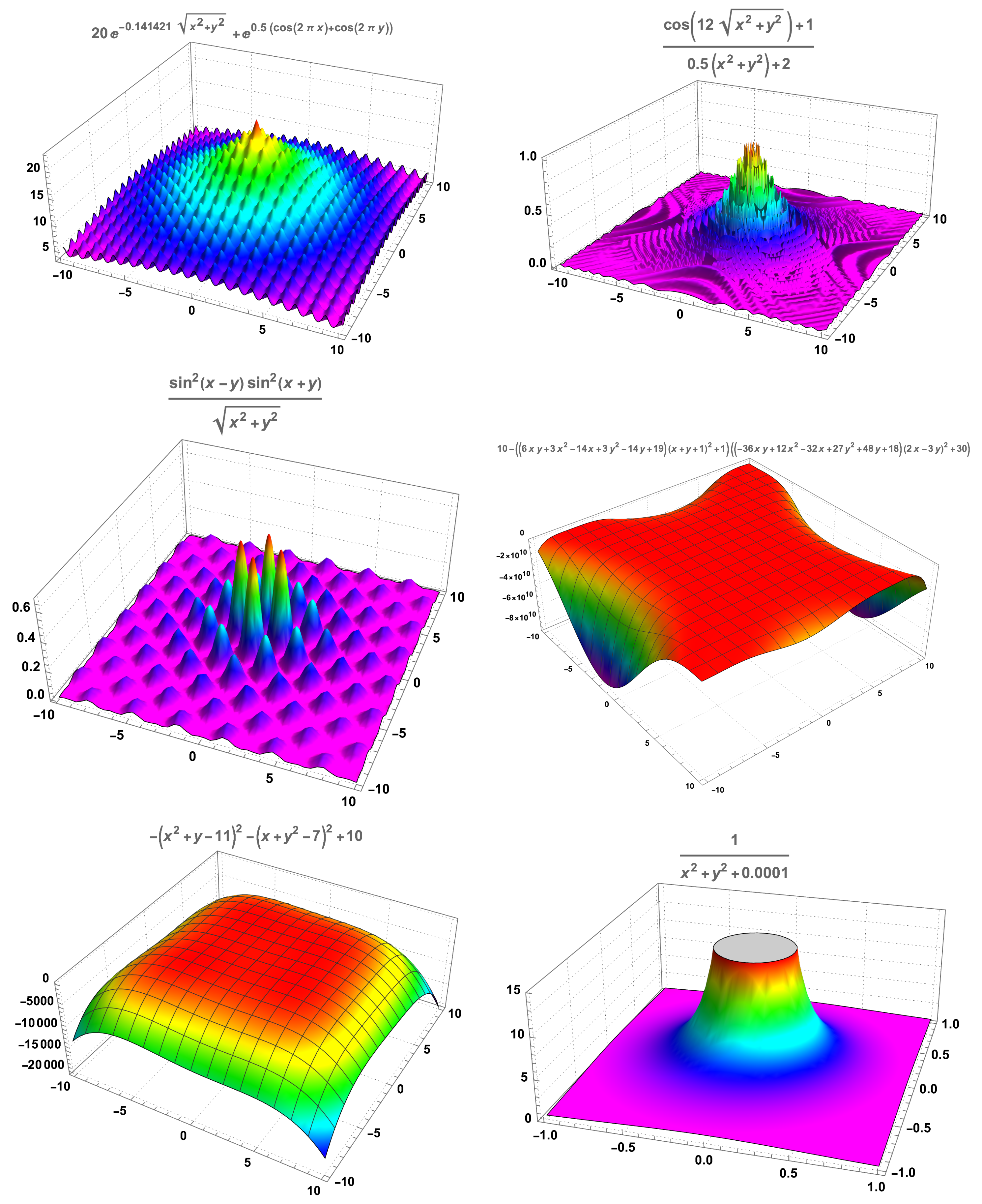
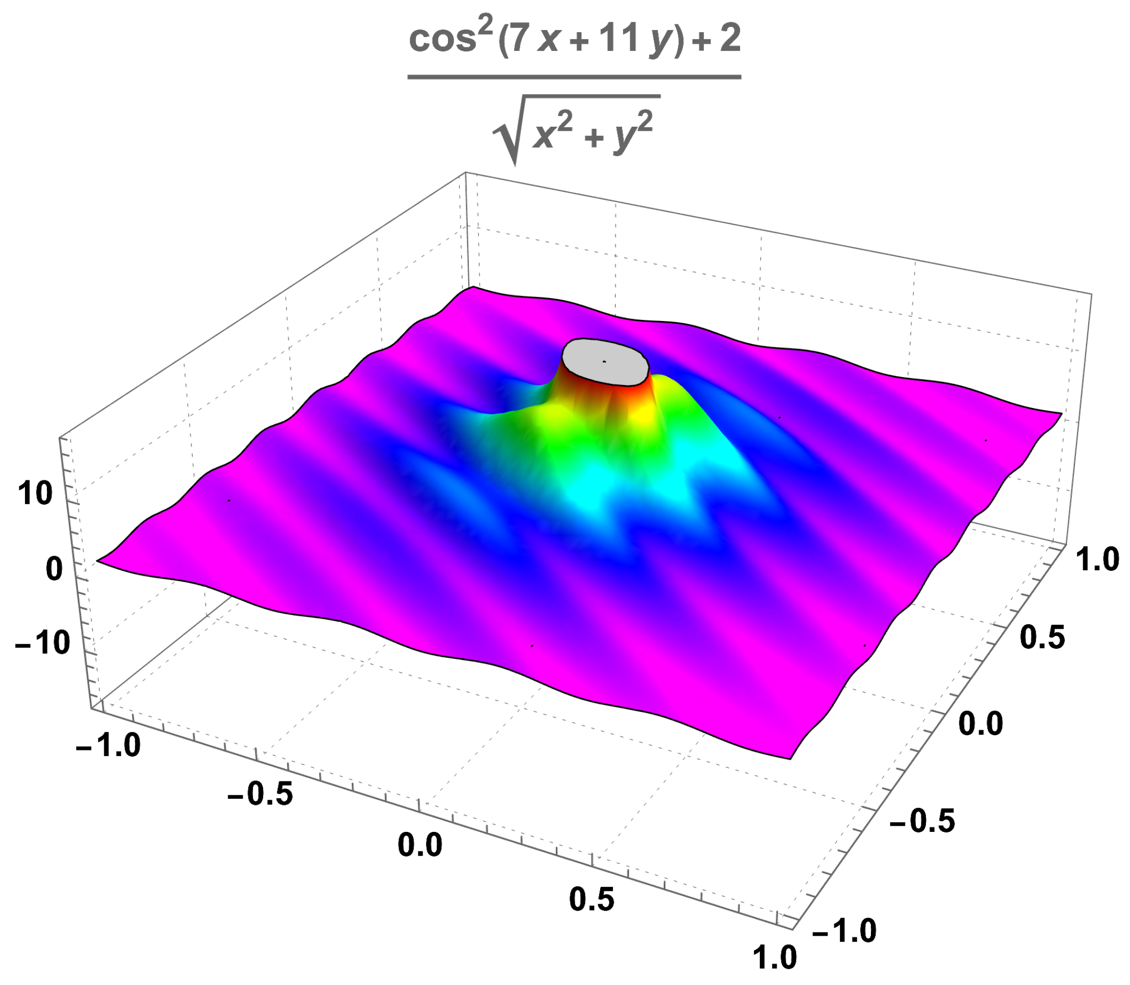
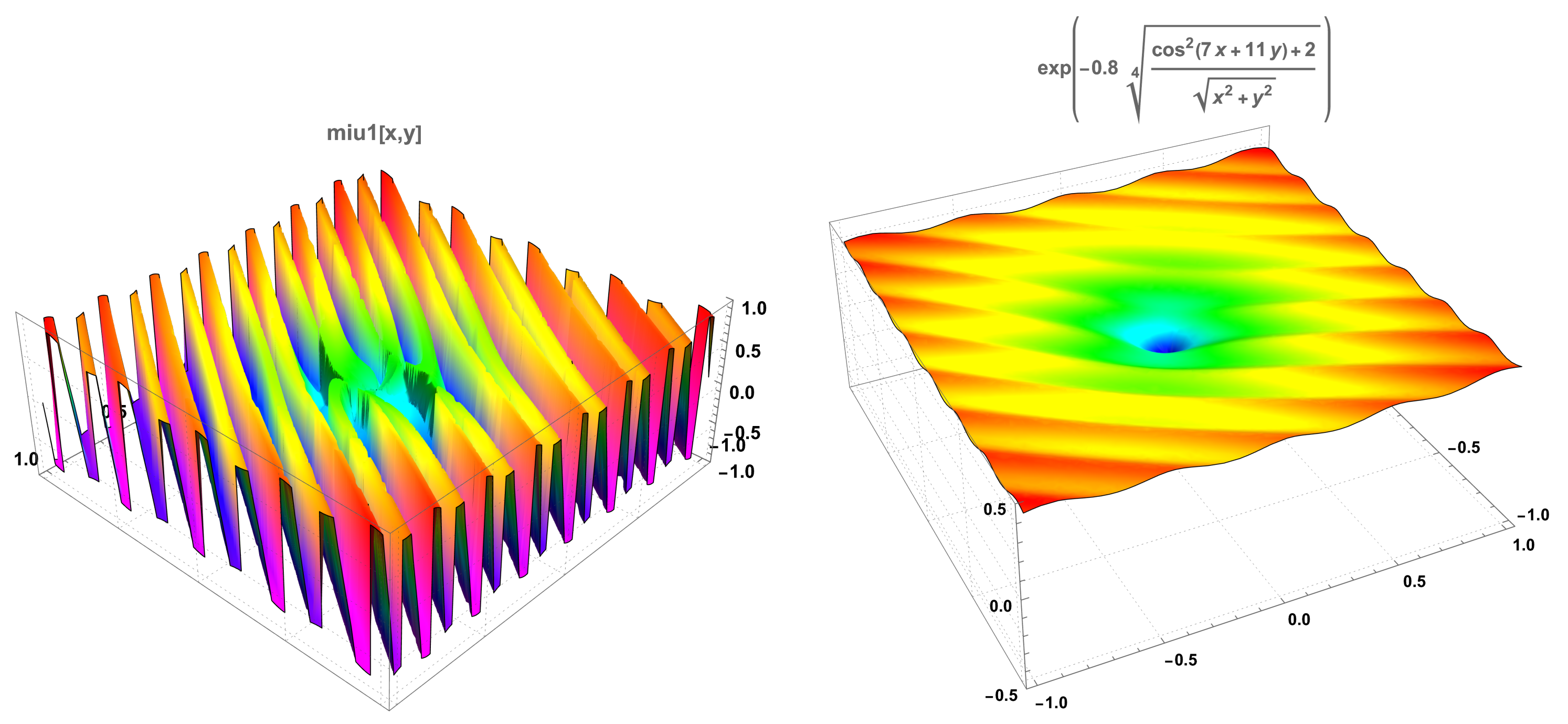
For each of the functions of two real variables studied (see Appendix A for additional information on these functions)—Ackley’s, drop-wave, Keane’s, Goldstein-Price’s, Himmelblau’s, and a nearly unbounded function—we determined, by Monte Carlo simulation, two lists of pairs of numbers, UU and VV. The list VV has 400 pairs of numbers, the first number of the pair being the time in seconds that the nonparallelised PRS algorithm overcomes $95\%$ of the known maximum of the function, at which point the simulation stopped, and the second number being the value attained at the moment the algorithm stopped. The list UU is similar to the list VV, but it contains the pair corresponding to the best performing kernel—among the four kernels of the machine used in the parallelised algorithm—regarding the value attained. In Appendix B, we detail the machine characteristics as well as the main code used in the computations both of the parallelised and the simple algorithms.

 2. 

We fitted a continuous bivariate distribution to both samples UU and VV, truncated to exact intervals of both time, the first marginal variate, and value, the second marginal variate. Then, using the probability density functions (PDF) of the marginals, denoted $f_{\mathrm{t}\mathrm{i}\mathrm{m}\mathrm{e}}^{\mathbf{UU}}$ and $f_{\mathrm{t}\mathrm{i}\mathrm{m}\mathrm{e}}^{\mathbf{VV}}$ for the first marginal and $f_{\mathrm{v}\mathrm{a}\mathrm{l}\mathrm{u}\mathrm{e}}^{\mathbf{UU}}$ and $f_{\mathrm{v}\mathrm{a}\mathrm{l}\mathrm{u}\mathrm{e}}^{\mathbf{VV}}$ for the second marginal of each of the two samples UU and VV, we determined two values of reference one $t_{\mathrm{r}\mathrm{e}\mathrm{f}}$ the time reference and the other $v_{\mathrm{r}\mathrm{e}\mathrm{f}}$ the value reference, such that:

$$f_{\mathrm{v}\mathrm{a}\mathrm{l}\mathrm{u}\mathrm{e}}^{\mathbf{UU}}\left(v_{\mathrm{r}\mathrm{e}\mathrm{f}}\right)=f_{\mathrm{v}\mathrm{a}\mathrm{l}\mathrm{u}\mathrm{e}}^{\mathbf{VV}}\left(v_{\mathrm{r}\mathrm{e}\mathrm{f}}\right) \mathrm{a}\mathrm{n}\mathrm{d} f_{\mathrm{time}}^{\mathbf{UU}}\left(t_{\mathrm{r}\mathrm{e}\mathrm{f}}\right)=f_{\mathrm{t}\mathrm{i}\mathrm{m}\mathrm{e}}^{\mathbf{VV}}\left(t_{\mathrm{ref}}\right).$$

(19)

We observe that, in some cases, $t_{\mathrm{r}\mathrm{e}\mathrm{f}}$ and $v_{\mathrm{r}\mathrm{e}\mathrm{f}}$ were not unique solutions of the equations $f_{\mathrm{v}\mathrm{a}\mathrm{l}\mathrm{u}\mathrm{e}}^{\mathbf{UU}}\left(v\right)=f_{\mathrm{v}\mathrm{a}\mathrm{l}\mathrm{u}\mathrm{e}}^{\mathbf{VV}}\left(v\right)$ in the variable v and $f_{\mathrm{t}\mathrm{i}\mathrm{m}\mathrm{e}}^{\mathbf{UU}}\left(t\right)=f_{\mathrm{t}\mathrm{i}\mathrm{m}\mathrm{e}}^{\mathbf{VV}}\left(t\right)$ in the variable t; whenever this situation occurred, we chose the solutions closest to the medians of the two distributions. Furthermore, in at least one of the cases, there was no solution of the equations with the PDF, and we used a solution of a similar equation but with the cumulative distribution functions.

 3. 

With the determined values of $t_{\mathrm{r}\mathrm{e}\mathrm{f}}$ and $v_{\mathrm{r}\mathrm{e}\mathrm{f}}$, we can immediately compute the conditional probabilities given by ${\mathbb{P}}_{\Vert }[V\ge v_{\mathrm{r}\mathrm{e}\mathrm{f}}|T\le t_{\mathrm{r}\mathrm{e}\mathrm{f}}]$ for the parallelised algorithm, V being the value variable and T the time marginal variable, and similarly, ${\mathbb{P}}_{\mid }[V\ge v_{\mathrm{ref}}|T\le t_{\mathrm{ref}}]$ for the nonparallelised algorithm. By analogy with Formula (14) in Theorem 3 and due to the choice of $t_{\mathrm{r}\mathrm{e}\mathrm{f}}$ and $v_{\mathrm{r}\mathrm{e}\mathrm{f}}$, we would expect to have:

$${\mathbb{P}}_{\Vert }[V\ge v_{\mathrm{ref}}|T\le t_{\mathrm{ref}}]\approx {\mathbb{P}}_{\mid }{[V\ge v_{\mathrm{ref}}|T\le t_{\mathrm{ref}}]}^r,$$

where r is the number of copies in the parallelised algorithm. As a consequence, with:

$$\widehat{r}:=\frac{log\left({\mathbb{P}}_{\Vert }[V\ge v_{\mathrm{ref}}|T\le t_{\mathrm{ref}}]\right)}{log\left({\mathbb{P}}_{\mid }[V\ge v_{\mathrm{ref}}|T\le t_{\mathrm{ref}}]\right)},$$

(20)

we expect to have $\widehat{r}\approx r$ in the examples given.

In

Table 1. Results comparing the parallelised and the nonparallelised algorithms.

Function	${\mathit{t}}_{\mathbf{ref}}$	Med. Time UU; VV	${\mathit{v}}_{\mathbf{ref}}$	Med. Value UU; VV	$\widehat{\mathit{r}}$
Ackley	1.01974	$2.315;0.320748$	22.1859	$22.3949;22.0619$	3.2257
Drop-wave	1.09633	$0.791884;0.67545$	0.981912	$0.990949;0.974948$	3.65206
Keane	0.0121573	$0.0114686;0.00892817$	0.659555	$0.66714;0.656837$	3.35966
Nearly unbounded	2.97751	$1.35259;6.05625$.	9784.74	$9901.14;9746.28$	3.89735
Goldstein-Price	3.52532	$1.25178;6.00467$	6.87869	$6.93984;6.82673$	3.34803
Himmelblau	0.25	$0.0163107;0.0135014$.	9.82452	$9.91097;9.73618$.	3.45038

, we present the results of the computations just described, with $r=4$ kernels, using the machine and code both presented in Appendix B. A first observation is that the result for the nearly unbounded function is the best among all functions tested. This kind of function will be the object of the results presented in Section 4. A second observation is that the median time values come from samples of repetitions of the algorithm both in the parallelised and nonparallelised versions; in the parallelised version, there are four times more repetitions than in the nonparallelised version, and being so, it is possible for the median times obtained with parallel algorithms to be sometimes worse than with the nonparallelised version.

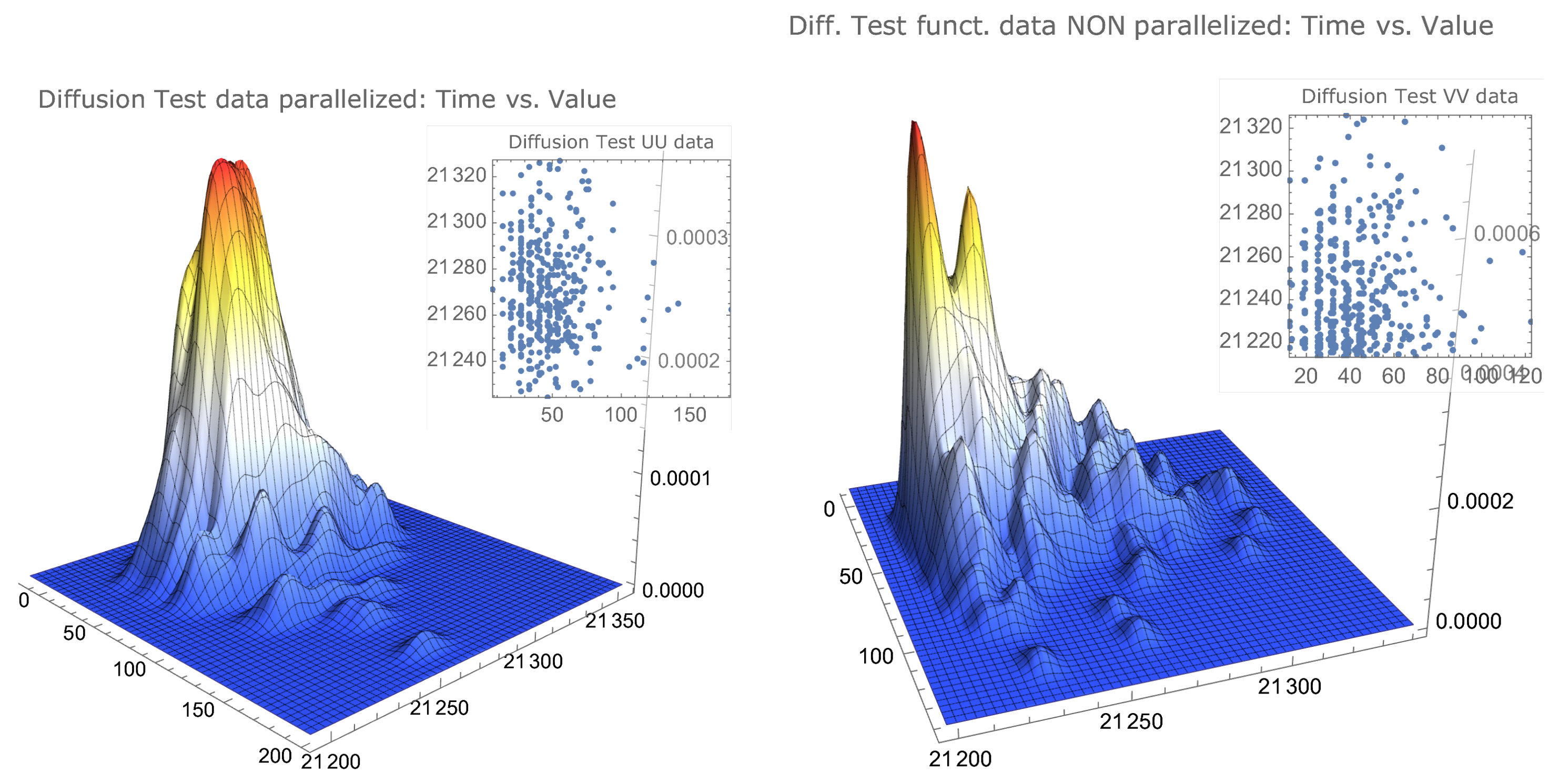
Remark 6

(Quantitative experimental validation of the advantage of a parallelisation of a pure random search). The results presented in Table 1 seem to substantiate the claim presented in Theorem 3, in Formula (14). In fact, it seems clear that, both for the examples of slightly modified well known test functions having several local maximums—Ackley’s, drop-wave, and Keane’s—and the functions attaining their maximums on a plateau-like surface—Goldstein–Price’s and Himmelblau’s—we obtain estimates of $r=4$, given by $\widehat{r}$, that can be considered acceptable, taking into account that, in the parallelised algorithm, efficiency losses occur in the distribution of tasks among kernels.

Remark 7

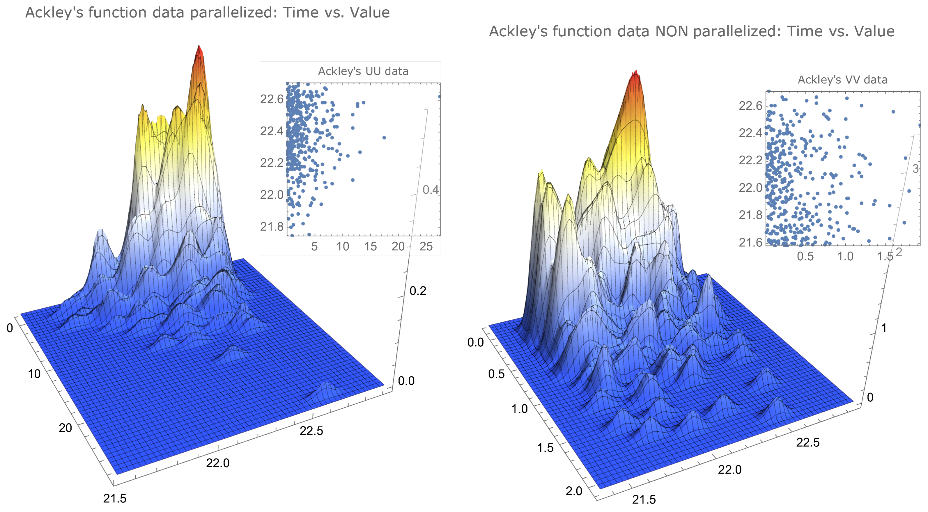
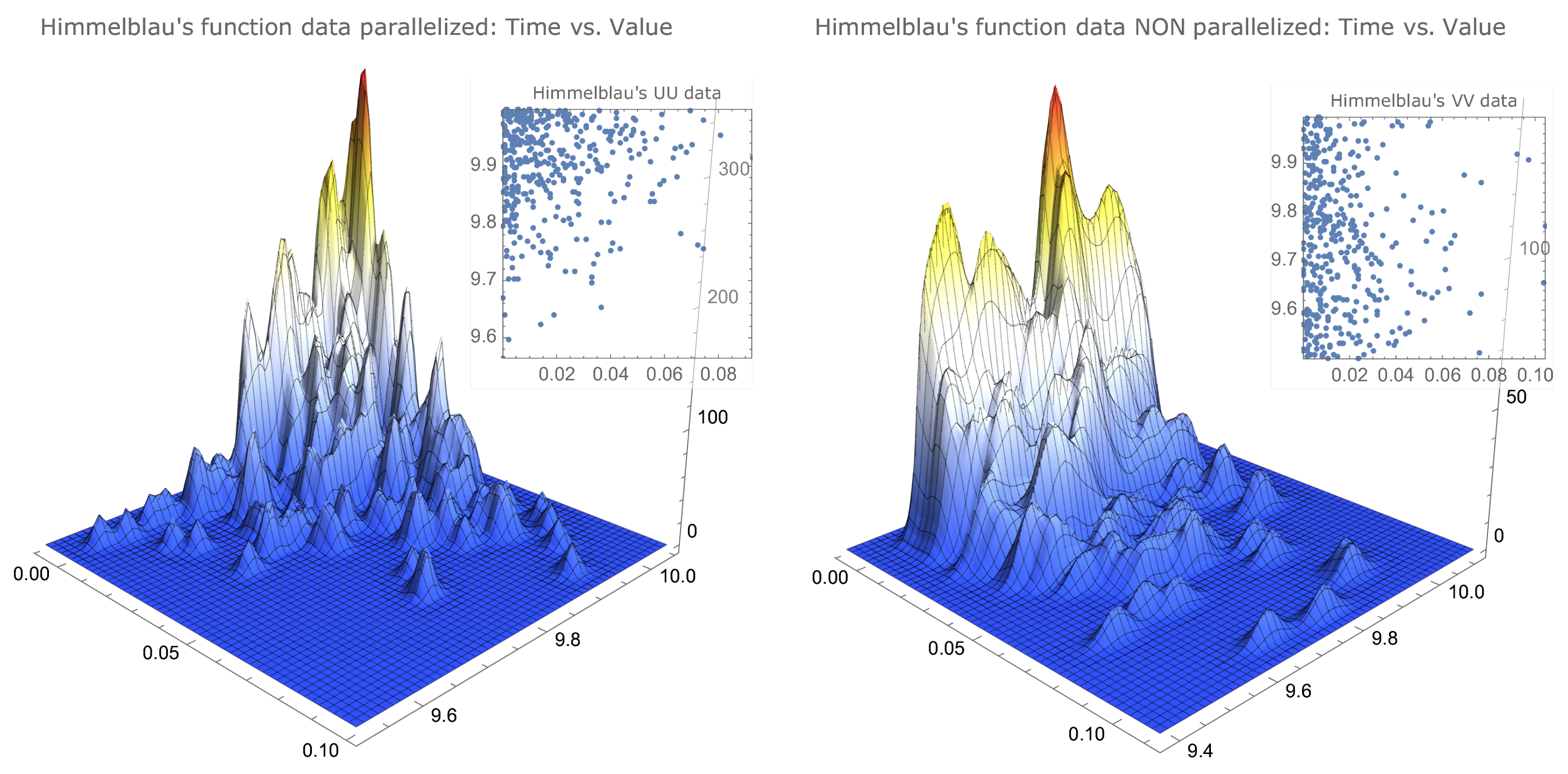
(Simulated data representations for examples of two types of functions). The simulated data that allowed us to determine the values of Table 1 can be visualised to provide a better insight of their characteristics. In Figure 1 and Figure 2, we compare the same data for functions that clearly differ in the maximum localisation characteristics. As already mentioned, the drop-wave function presents several local maxima, with some of these local maxima agglomerated together with the global maximum, and the Himmelblau’s function has its maximum—with four distinct maximisers—in a surface plateau.

There is a noticeable similarity between the parallelised data of both functions, as well as between the nonparallelised data of both functions.

However, there is a noticeable difference, for each function, between the parallelised data and the nonparallelised data. The parallelised data for both functions show a concentration on the upper left corner—less accentuated for Ackley’s function—that is, surrounding the best values in a way that can be described as: closest to the true maximum and smallest times—more noticeable for Himmelblau’s function—while the nonparallelised data, for both functions, appear to be uniformly distributed in the interval $[95\%max,max]$, also being more scattered in the time variable.

4. On a Martingale Diffusion Type Algorithm for Global Optimisation

In this section, we propose an algorithm for global optimisation based on the maximum principle for strictly elliptic operators. Let us take as an example a harmonic function on an open and bounded domain with regular boundary; this function belongs to the kernel of the Laplacian operator. It is well known that such a function attains its maximum on the boundary. Consider the diffusion naturally associated with the Laplacian. The algorithm we propose consists of running the diffusion on the domain until it touches the boundary; then, by a Feynman–Kǎc-type result, we can obtain the maximum value of the function. This algorithm is suited for nearly unbounded functions. We next detail the general idea of our approach.

4.1. On the Maximum Principle for Strictly Elliptic Operators

Consider a function $f:\overline{\mathcal{D}}\subset {\mathbb{R}}^2⟶\mathbb{R}$, where $\mathcal{D}$ is a bounded open set with a regular boundary $\partial \mathcal{D}$. We consider the following two global optimisation goals for the function f over the compact $\overline{\mathcal{D}}$.

 (a) 

Determination of ${sup}_{(x_1,x_2)\in \overline{\mathcal{D}}}f(x_1,x_2)=:M_{f,\overline{\mathcal{D}}}$.

 (b) 

Determination of the set of maximisers $\left\{(x_1,x_2)\in \overline{\mathcal{D}}:f(x_1,x_2)=:M_{f,\overline{\mathcal{D}}}\right\}$.

We will consider the following regularity hypothesis of f over $\overline{\mathcal{D}}$.

 (A1) 

$f\in {\mathcal{C}}^2\left(\mathcal{D}\right)$ (f is twice differentiable on $\mathcal{D}$, and the second differential is continuous) and $f\in {\mathcal{C}}^0\left(\overline{\mathcal{D}}\right)$ (f is continuous in $\overline{\mathcal{D}}$).

We consider $(\mathsf{\Omega },\mathcal{F},\mathbb{P})$ a complete probability space and ${\mathbb{B}}^1={\left(B_t^1\right)}_{t\ge 0}$ and ${\mathbb{B}}^2={\left(B_t^2\right)}_{t\ge 0}$ two independent Brownian processes on $(\mathsf{\Omega },\mathcal{F},\mathbb{P})$. Let $\mathbb{F}={\left({\mathcal{F}}_t\right)}_{t\ge 0}$ be the natural filtration generated by both ${\mathbb{B}}^1$ and ${\mathbb{B}}^2$, which we assume to be complete and right-continuous. The first ingredient in the elaboration of our algorithm is a two-dimensional diffusion process ${\left(Y_t\right)}_{t\ge 0}\equiv {(Y_t^1,Y_t^2)}_{t\ge 0}$, that is, a strong solution of the following system of stochastic differential equations:

$$\left\{\begin{array}{c}\hfill d{Y}_t^1={\mu }_1\left(Y_t\right)dt+{\sigma }_1\left(Y_t\right)d{B}_t^1,Y_0^1\in \mathbb{R}\\ \hfill d{Y}_t^2={\mu }_2\left(Y_t\right)dt+{\sigma }_2\left(Y_t\right)d{B}_t^2,Y_0^2\in \mathbb{R}.\end{array}\right.$$

(21)

We will suppose that the coefficients ${\mu }_1,{\sigma }_1$ and ${\mu }_2,{\sigma }_2$ have the necessary regularity to ensure the existence of a strong solution (see Remark 9 on validity of this hypothesis).

In order to guarantee some useful convergence properties, we assume the following hypothesis.

 (A2) 

The process ${\left(f\left(Y_t\right)\right)}_{t\ge 0}$ is a $\mathbb{F}$-martingale.

As a result of an application of Ito’s formula (as in ([45], pp. 32–33)), we can identify a partial differential operator that will impose further constraints on the coefficients of the diffusions in Formula (21). In fact, we have:

$$\begin{array}{cc}\hfill df\left(Y_t\right)& =\left[{\mu }_1\left(Y_t\right)\frac{\partial f}{\partial x_1}\left(Y_t\right)+{\mu }_2\left(Y_t\right)\frac{\partial f}{\partial x_2}\left(Y_t\right)+\frac{1}{2}\left(\frac{{\partial }^{2}f}{\partial x_1^2}\left(Y_t\right){\sigma }_1^2\left(Y_t\right)+\frac{{\partial }^{2}f}{\partial x_2^2}\left(Y_t\right){\sigma }_2^2\left(Y_t\right)\right)\right]dt+\hfill \\ & +\left(\frac{\partial f}{\partial x_1}\left(Y_t\right){\sigma }_1\left(Y_t\right)d{B}_t^1+\frac{\partial f}{\partial x_2}\left(Y_t\right){\sigma }_2\left(Y_t\right)d{B}_t^2\right),\hfill \end{array}$$

(22)

and in order for ${\left(f\left(Y_t\right)\right)}_{t\ge 0}$ to be a martingale, the sum of the terms that constitute the $dt$ coefficient in Formula (22) has to vanish. Furthermore, if we consider the operator defined for $h:(x_1,x_2)\in \mathcal{D}\mapsto h(x_1,x_2)\in \mathbb{R}$, $h\in {\mathcal{C}}^2\left(\mathcal{D}\right)$, by:

$$\mathcal{L}\left(h\right)(x_1,x_2):=\sum _{i=1}^2{\mu }_i(x_1,x_2)\frac{\partial h}{\partial x_i}(x_1,x_2)+\frac{1}{2}\sum _{i=1}^2{\sigma }_i^2(x_1,x_2)\frac{{\partial }^{2}h}{\partial x_i^2}(x_1,x_2),$$

(23)

we should have $\mathcal{L}\left(f\right)\equiv 0$ in $\mathcal{D}$; a condition denominated f is $\mathcal{L}$ harmonic on $\mathcal{D}$ (see [46], p. 47).

Now, in order to ensure a Feynman–Kǎc-type representation result, we assume the following hypothesis:

 (A3) 

The operator $\mathcal{L}$ is strictly elliptic on $\mathcal{D}$, that is,

$$\forall \mathit{x}=(x_1,x_2)\in \mathcal{D}\exists \Lambda \left(\mathit{x}\right)>0\forall z_1,z_2\in \mathbb{R},\sum _{i,j=1}^2{\sigma }_i\left(\mathit{x}\right){\sigma }_j\left(\mathit{x}\right)z_i{z}_j\ge \Lambda \left(\mathit{x}\right)\sum _{i=1}^2{z}_i^2.$$

(24)

The following result, which we quote from ([46], p. 46), gives a representation of the solutions of a well posed problem with operator $\mathcal{L}$ using the diffusion ${\left(Y_t\right)}_{t\ge 0}$.

Theorem 4

(A Feynman–Kǎc-type representation of the solution of a Dirichlet problem). Let u be a solution of the Dirichlet problem for the operator $\mathcal{L}$ in Formula (23) associated with the function f in $\mathcal{D}$, that is:

• $u\in {\mathcal{C}}^2\left(\mathcal{D}\right)$ and $u\in {\mathcal{C}}^0\left(\overline{\mathcal{D}}\right)$.
• $\mathcal{L}\left(u\right)\equiv 0$ in $\mathcal{D}$ and $u\equiv f$ in $\partial \mathcal{D}$.

Then, with ${\tau }_{\mathcal{D}}$, theexit timeof ${\left(Y_t\right)}_{t\ge 0}$ from $\mathcal{D}$, that is, ${\tau }_{\mathcal{D}}:=inf\left\{t>0:Y_t\notin \mathcal{D}\right\}$, we have the following representation:

 (a) 

${\tau }_{\mathcal{D}}<+\infty$ almost surely (see also ([47], p. 324)).

 (b) 

For all $\mathit{x}\in \mathcal{D}$, we have that $u\left(\mathit{x}\right)={\mathbb{E}}^{\mathit{x}}\left[f\left(Y_{{\tau }_{\mathcal{D}}}\right)\right]$, with ${\mathbb{E}}^{\mathit{x}}$ being the expectation with respect of the law of ${\left(Y_t\right)}_{t\ge 0}$ given as a solution of the diffusion system in Formula (21) with initial condition $\mathit{x}$.

As a consequence of the statement (b) of Theorem 4, we have the following maximum principle that is crucial for our algorithm proposal.

Theorem 5

(A maximum principle application). Consider the notations and conditions of Theorem 4, and suppose that f is $\mathcal{L}$ harmonic in $\mathcal{D}$, and moreover, that f is a solution of the Dirichlet problem for the operator $\mathcal{L}$, associated with the function f in $\mathcal{D}$, that is:

• $f\in {\mathcal{C}}^2\left(\mathcal{D}\right)$ and $f\in {\mathcal{C}}^0\left(\overline{\mathcal{D}}\right)$.
• $\mathcal{L}\left(f\right)\equiv 0$ in $\mathcal{D}$, and obviously, $f\equiv f$ in $\partial \mathcal{D}$.

We then have, by the conclusion of Theorem 4:

$$\forall \mathit{x}\in \overline{\mathcal{D}}\left|f\left(\mathit{x}\right)\right|\le \underset{\mathbf{y}\in \partial \mathcal{D}}{sup}\left|f\left(\mathbf{y}\right)\right|.$$

Proof. 

Since, by the representation formula, we have for all $\mathit{x}\in \mathcal{D}$ that $f\left(\mathit{x}\right)={\mathbb{E}}^{\mathit{x}}\left[f\left(Y_{{\tau }_{\mathcal{D}}}\right)\right]$, we can conclude that:

$$\left|f\left(\mathit{x}\right)\right|=|{\mathbb{E}}^{\mathit{x}}\left[f\left(Y_{{\tau }_{\mathcal{D}}}\right)\right]|\le {\mathbb{E}}^{\mathit{x}}\left[|f\left(Y_{{\tau }_{\mathcal{D}}}\right)|\right]\le {\mathbb{E}}^{\mathit{x}}\left[\underset{\mathbf{y}\in \partial \mathcal{D}}{sup}\left|f\left(\mathbf{y}\right)\right|\right]=\underset{\mathbf{y}\in \partial \mathcal{D}}{sup}\left|f\left(\mathbf{y}\right)\right|,$$

and the conclusion now follows the hypothesis $f\in {\mathcal{C}}^0\left(\overline{\mathcal{D}}\right)$.    □

Remark 8.

Let us summarise the main ideas we are pursuing. We link the function f to a two-dimensional diffusion by means of a strictly elliptic differential operator of second order having as coefficients the diffusion coefficients, for which f is a solution of a Dirichlet problem. The representation Theorem 4 shows that, if we start the diffusion anywhere on the domain of f, and then we wait until the diffusion hits the boundary, we will have that the value of the function f at this point is a candidate to the maximum of the function in the closure of its definition domain.

4.2. The Practical Implementation of the Algorithm

Following the main idea exposed in Remark 8, we need to determine the coefficients of the diffusions in such a way that we have $\mathcal{L}\left(f\right)\equiv 0$. For that purpose, we do the following.

• We assume that, as f grows, the volatilities of the diffusions should decrease, and so we consider, for instance,

  $${\sigma }_i=e^{-{\alpha }_i{\left|f\right|}^{{\beta }_i}},i=1,2;{\alpha }_i,{\beta }_i>0,$$

  (25)

  with ${\alpha }_i$ and ${\beta }_i$ to be chosen appropriately depending on f, its domain of definition $\mathcal{D}$, and possibly also in an adaptive way in the algorithm.
• We consider two functions $g_i:(x_1,x_2)\in \mathcal{D}\mapsto g_i(x_1,x_2)\in \mathbb{R}$, $g_i\in {\mathcal{C}}^1\left(\mathcal{D}\right)$, for $i=1,2$, such that:

  $$\frac{\partial f}{\partial x_i}=g_{i}f.$$

  (26)
  We observe that, by Schwarz’s theorem, we have that $\partial g_1/\partial x_2=\partial g_2/\partial x_1$.
• In order to determine the drift coefficients of the diffusions, we may observe that, for $f\ne 0$, we have that $\mathcal{L}\left(f\right)=0$ if and only if:

  $${\mu }_1{g}_1+{\mu }_2{g}_2+\left(\frac{\partial g_1}{\partial x_1}+g_1^2\right)\frac{{\sigma }_1^2}{2}+\left(\frac{\partial g_2}{\partial x_2}+g_2^2\right)\frac{{\sigma }_2^2}{2}=0,$$

  as a result of Formula (23) and of the previous determinations. This equality can be achieved by taking, for instance, for $i=1,2$,

  $${\mu }_i=-\left(\frac{\partial g_i}{\partial x_i}+g_i^2\right)\frac{{\sigma }_i^2}{2g_i},$$

  (27)

  an expression that is determined as soon as the functions $g_i$ are determined.
• We can consider the equally spaced Euler–Maruyama discretisation (see ([48], p. 305) or ([49], p. 152)) of the diffusions in Formula (21), that is, for $i=1,2$,

  $$\left\{\begin{array}{cc}{Y}_{n+1}^i=Y_n^i+{\mu }_i\left((Y_n^1,Y_n^2)\right)\Delta t+{\sigma }_i\left((Y_n^1,Y_n^2)\right)\sqrt{\Delta t}{Z}_n^i\hfill & n\ge 0\hfill \\ Y_0^i=x_i,\hfill & \end{array}\right.$$

  (28)
  $\Delta t$ being the discretisation step, with $Y_n^i\equiv Y_{\Delta tn}^i$ and the sequence ${\left(Z_n^i\right)}_{n\ge 0}$ being a sequence of independent and identically distributed random variables with a standard Gaussian random variable, that is, $Z⌢\mathcal{N}(0,1)$.

The effectiveness of the practical implementation of the algorithm is conditioned to the existence of strong solutions of the system of SDE given in Formula (21), having the drifts given by Formula (27) and volatilities given by Formula (25). A first observation is that, as a consequence of Formula (26) and of Formula (27), we have, for $i=1,2$, that:

$${\mu }_i=-\frac{\frac{{\partial }^{2}f}{\partial x_i^2}}{\frac{\partial f}{\partial x_i}}.\frac{{\sigma }_i^2}{2}.$$

(29)

Thus, if $\frac{\partial f}{\partial x_i}$ is bounded away from zero, that is, if $\frac{\partial f}{\partial x_i}\ge a>0$, and if $\frac{\partial f}{\partial x_i}\in {\mathcal{C}}^0\left(\overline{\mathcal{D}}\right)$, we have that ${\mu }_i$ is a continuous function over the compact $\overline{\mathcal{D}}$ and so is both uniformly continuous and bounded in $\overline{\mathcal{D}}$. A second observation is that, with the choice ${\sigma }_1={\sigma }_2>ϵ>0$ in Formula (25) we have that, for

$$\begin{array}{cc}\hfill \sum _{i,j=1}^2{z}_i{z}_j{\sigma }_i{\sigma }_j& ={(z_1{\sigma }_1+z_2{\sigma }_2)}^2={\sigma }_1^2{(z_1+z_2)}^2\ge {\sigma }_1^2|z_1+z_2{|}^2\ge {\sigma }_1^2{\left||z_1|-|z_2|\right|}^2\ge \hfill \\ \hfill & \ge {\sigma }_1^{2}max\left(\right|z_1{|}^2,|z_2{|}^2)\ge \frac{{\sigma }_1^2}{2}(z_1^2+z_2^2)\ge \frac{{ϵ}^2}{2}(z_1^2+z_2^2),\hfill \end{array}$$

and so the operator defined in Formula (23) is strictly elliptic—even uniformly strictly elliptic—according to Formula (24). We now need an existence result for the system of stochastic differential equations given in Formula (21) having the drifts given by Formula (27) and volatilities given by Formula (25). For that purpose, we quote the following version of the celebrated Yamada–Watanabe theorem (see ([50], pp. 40–41)).

Theorem 6

(Yamada and Watanabe 1971). Suppose that μ and σ are progressively measurable and bounded and satisfy the following hypothesis.

 (1) 

There exists ${\rho }_1:[0,+\infty [\mapsto [0,+\infty [$, anincreasingcontinuous function, such that ${\rho }_1\left(0\right)=0$, such that:

$$\forall t,x,y∥\sigma (t,x)-\sigma (t,y)∥\le {\rho }_1\left(\right|x-y\left|\right)and\underset{ϵ\to 0}{lim}{\int }_{ϵ}\frac{du}{{\rho }_1\left(u\right)}=+\infty .$$

 (2) 

There exists ${\rho }_2:[0,+\infty [\mapsto [0,+\infty [$, anincreasing concavefunction, such that ${\rho }_2\left(0\right)=0$, such that:

$$\forall t,x,y\left(\mu (t,x)-\mu (t,y)\right)\le {\rho }_2\left(\right|x-y\left|\right)and\underset{ϵ\to 0}{lim}{\int }_{ϵ}\frac{du}{{\rho }_2\left(u\right)}=+\infty .$$

Then, for any random variable Z, where $t_0\in [0,T]$, the following stochastic differential equation

$$\left\{\begin{array}{cc}d{X}_t=\mu (t,X_t)dt+\sigma (t,X_t)d{B}_t,\hfill & t\in [t_0,T],\hfill \\ X_{t_0}=Z,\hfill \end{array}\right.$$

(30)

has a strong solution and uniqueness in law holds.

Remark 9

(On the existence and unicity of the process ${\left(Y_t\right)}_{t\ge 0}$ defining the diffusion algorithm). Despite the fact that, in general, we do not have the sub-linear growth of the coefficients that, together with the Lipschitz character of these coefficients, ensures existence and unicity of a strong solution in the context of the classical Ito’s theorem, we may nevertheless conclude that the system of stochastic differential equations given in Formula (21), having the drifts given by Formula (27) and volatilities given by Formula (25), has a strong solution that is unique in law; this happens as long as we force the solution process to stay on a compact set contained in $\mathcal{D}$. In fact, by the regularity properties imposed on f, we have that ${\sigma }_i\in {\mathcal{C}}^2\left(\mathcal{D}\right)$ and ${\sigma }_i\in {\mathcal{C}}^0\left(\overline{\mathcal{D}}\right)$; thus, by the mean value theorem, on any compact set contained in $\mathcal{D}$, we have that ${\sigma }_i$ has a bounded derivative, and so it verifies a Lipschitz condition, which implies that it satisfies hypothesis (1) of Theorem 6. Moreover, as pointed out above, the regularity properties imposed on f also imply that the term not containing ${\sigma }_i$ in Formula (27) is bounded, and so the drifts are also Lipschitz on any compact set contained in $\mathcal{D}$ by virtue of the same property that the term ${\sigma }_i$—in Formula (27)—has. The practical implementation of the algorithm in Section 4.3 considers that the diffusion process is restrained to a compact set contained in the maximal open set where the function f is defined.

Remark 10

(On the convergence of the Euler–Maruyama discretisation). The equally spaced Euler–Maruyama discretisation that we propose in Formula (28) converges weakly under a very general hypothesis, as stated in Proposition 4.58 in ([49], p. 146). This is a consequence of the regularity of the coefficients—${\mu }_i$ is continuous, and ${\sigma }_i$ has the same regularity as f—and the fact that the strong solution of a SDE given by an Ito integral, with continuous coefficients, is a continuous function of the Brownian process. Nevertheless, the question of the strong convergence and of the rate of convergence of the Euler–Maruyama discretisation should be addressed for each particular case of the function f studied.

Remark 11

(The martingale diffusion type algorithm). A simplified scheme describing the martingale diffusion-type algorithm is the following. The actual implementations in Mathematica ™(see [51]) for both the parallelised and nonparallelised versions are presented in Listing A4 and Listing A3, respectively.

• STEP 1:
  • CHOOSE Tolerance error $ϵ>0$ and upper bound A.
• STEP 2:
  • CHOOSE$(x_1,x_2)\in \overline{\mathcal{D}}$ at random uniformly;
  • DO:$Y_0^i=x_i$, for $i=1,2$ and $M_1=f(x_1,x_2)$
• STEP 3:
  • DO: compute iteratively $(Y_n^1,Y_n^2)$ for $n\ge 1$ according to Formula (28);
  • IF$f(Y_n^1,Y_n^2)>M_1$DO:$M_1=f(Y_n^1,Y_n^2)>M_1$
  • UNTIL either one of the following stopping criteria is verified:
    • stop at $n=n_0$ such that: $(Y_{n_0}^1,Y_{n_0}^2)\notin \mathcal{D}$ or,
    • stop at n such that: $|Y_n^1-Y_{n-1}^1|+|Y_n^2-Y_{n-1}^2|<ϵ$ and
    • either $|f\left(Y_n\right)-f\left(Y_{n-1}\right)|<ϵ$ or $|f\left(Y_n\right)|>A$;
• STOP or GO TO STEP 2 with new $M_2$ that must be compared with $M_1$.

We observe thatSTEP 2in the algorithm is of the pure random search kind. Being so, if the algorithm is parallelisable, the results of Section 2.2 can be applied. In the parallelised version, there will be an extra step added to the above pseudo-code for collecting the times and values of each of the four copies of the algorithm.

We now prove that the algorithm we just described in the simplified scheme above is parallelizable according to Definition 4.

Theorem 7

(Parallelisation of martingale diffusion-type algorithm). Let the process ${\left(Y_t\right)}_{t\ge 0}$ be given by the set of two diffusions in Formula (21). Suppose that the process ${\left(f\left(Y_t\right)\right)}_{t\ge 0}$ is such that Hypothesis (A1), (A2), and (A3) hold. Then, the process ${\left(f\left(Y_t\right)\right)}_{t\ge 0}$ is a uniformly integrable martingale, and so it converges, almost surely and in $L^1$, to a random variable ${\mathbb{Y}}_{\infty }^f$. Moreover, if $f\ge 0$, we have that:

 (a) 

the well defined random variable $f\left(Y_{{\tau }_{\mathcal{D}}}\right)$ is a weak solution of the global optimisation problem for f in $\overline{\mathcal{D}}$;

 (b) 

the algorithm described in Remark 11 is parallelizable.

Proof. 

It is clear that, as $f\in {\mathcal{C}}^0\left(\overline{\mathcal{D}}\right)$ that for every $p>1$, we have that:

$$\underset{t\ge 0}{sup}\mathbb{E}\left[|f\left(Y_t\right){|}^p\right]<+\infty ,$$

and so the process ${\left(f\left(Y_t\right)\right)}_{t\ge 0}$ is uniformly integrable (see, for instance, ([41], p. 29)); moreover, this process being a martingale in continuous time it converges almost surely and in $L^1$ to a random variable that closes the martingale (see, for instance, ([41], p. 88)). From statement (b) in Theorem 4, it follows that the random variable $f\left(Y_{{\tau }_{\mathcal{D}}}\right)$ is well defined. Now, without loss of generality, we may suppose that $f\ge 0$. Now, again by Theorem 5 and its proof, we have that:

$$\forall x\in \overline{\mathcal{D}}f\left(x\right)\le \underset{y\in \partial \mathcal{D}}{sup}f\left(y\right)={\mathbb{E}}^{\mathit{x}}\left[f\left(Y_{{\tau }_{\mathcal{D}}}\right)\right].$$

Since $\mathcal{D}$ is bounded, we recall Definition 2 of the essential supremum of f over the compact set $\overline{\mathcal{D}}$,

$${\alpha }_f=inf\left\{t:f\left(x\right)\le t,\lambda \mathrm{a}\mathrm{l}\mathrm{m}\mathrm{o}\mathrm{s}\mathrm{t} \mathrm{e}\mathrm{v}\mathrm{e}\mathrm{r}\mathrm{y}\mathrm{w}\mathrm{h}\mathrm{e}\mathrm{r}\mathrm{e} \mathrm{o}\mathrm{n} \overline{\mathcal{D}}\right\},$$

from which is clear that

$$0\le {\alpha }_f\le =\underset{y\in \overline{\mathcal{D}}}{sup}f\left(y\right)=\underset{y\in \partial \mathcal{D}}{sup}f\left(y\right)={\mathbb{E}}^{\mathit{x}}\left[f\left(Y_{{\tau }_{\mathcal{D}}}\right)\right],$$

(31)

and so Assertion (a) of the theorem is proved. From Formula (28), it is clear that, for $i=1,2$, the law of $Y_{n+1}^i$ depends only on the law of the random variable $(Z_0^i,Z_1^i,\cdots ,Z_n^i)$, and so the same happens with the law of the integer valued hitting time of $\partial \mathcal{D}$, that is, ${\tau }_{\mathcal{D}}^{\Delta }:=inf\left\{n>0:(Y_n^1,Y_n^2)\notin \mathcal{D}\right\}$; we observe that, almost surely, we have:

$$\underset{\Delta t⟶0}{lim}{\tau }_{\mathcal{D}}^{\Delta }={\tau }_{\mathcal{D}}.$$

(32)

In fact, since we have that ${\tau }_{\mathcal{D}}=inf\left\{t>0:Y_t\in \partial \mathcal{D}\right\}$, we may state:

• $\forall t<{\tau }_{\mathcal{D}},Y_t\in \mathcal{D}$;
• and for almost all $\omega \in \mathsf{\Omega }$, we have that:

  $$\forall \Delta t>0,\exists n_{\Delta }=n_{\Delta }\left(\omega \right),{\tau }_{\mathcal{D}}\left(\omega \right)\in [n_{\Delta }\Delta t,(n_{\Delta }+1)\Delta t[.$$

  (33)

Since ${\tau }_{\mathcal{D}}^{\Delta }=inf\left\{m>1:Y_{m\Delta t}\notin \mathcal{D}\right\}$, we now have for the hitting time of $\partial \mathcal{D}$ by the discretised process that ${\tau }_{\mathcal{D}}^{\Delta }\le (n_{\Delta }+1)\Delta t$ by force of Formula (33); moreover, the following dichotomy applies:

$$\left\{\begin{array}{cc}\mathrm{i}\mathrm{f} {\tau }_{\mathcal{D}}\left(\omega \right)=n_{\Delta }\Delta t,\hfill & \mathrm{t}\mathrm{h}\mathrm{e}\mathrm{n} {\tau }_{\mathcal{D}}^{\Delta }\left(\omega \right)={\tau }_{\mathcal{D}}\left(\omega \right),\hfill \\ \mathrm{i}\mathrm{f} {\tau }_{\mathcal{D}}\left(\omega \right)>n_{\Delta }\Delta t\hfill & \mathrm{t}\mathrm{h}\mathrm{e}\mathrm{n} {\tau }_{\mathcal{D}}^{\Delta }\left(\omega \right)\ge n_{\Delta }\Delta t,\hfill \end{array}\right.$$

and in any case, we have $|{\tau }_{\mathcal{D}}\left(\omega \right)-{\tau }_{\mathcal{D}}^{\Delta }\left(\omega \right)|<\Delta t$, as claimed. Now, if we redefine the discretised algorithm ${\left({\tilde{Y}}_n\right)}_{n\ge 0}$ by:

$${\tilde{Y}}_n=\left\{\begin{array}{cc}{Y}_n\hfill & \mathrm{f}\mathrm{o}\mathrm{r} n<{\tau }_{\mathcal{D}}^{\Delta }\hfill \\ Y_{{\tau }_{\mathcal{D}}^{\Delta }}\hfill & \mathrm{f}\mathrm{o}\mathrm{r} n\ge {\tau }_{\mathcal{D}}^{\Delta },\hfill \end{array}\right.$$

we will have

$$\underset{n\to +\infty }{lim}{d}_{KF}(f\left({\tilde{Y}}_n\right),f\left(Y_{{\tau }_{\mathcal{D}}^{\Delta }}\right))=0.$$

(34)

Moreover, we observe that:

$$\begin{array}{cc}\hfill ||{\mathbb{E}}^{\mathit{x}}\left[f\left(Y_{{\tau }_{\mathcal{D}}^{\Delta }}\right)\right]|-|{\mathbb{E}}^{\mathit{x}}\left[f\left(Y_{{\tau }_{\mathcal{D}}}\right)\right]||& \le {\mathbb{E}}^{\mathit{x}}\left[|f\left(Y_{{\tau }_{\mathcal{D}}^{\Delta }}\right))-f\left(Y_{{\tau }_{\mathcal{D}}}\right)|\right]\le \hfill \\ \hfill & \le {\mathbb{E}}^{\mathit{x}}\left[|f\left(Y_{{\tau }_{\mathcal{D}}^{\Delta }}\right))-f\left({\tilde{Y}}_n\right)|\right]+{\mathbb{E}}^{\mathit{x}}\left[|f\left({\tilde{Y}}_n\right)-f\left(Y_{{\tau }_{\mathcal{D}}}\right)|\right].\hfill \end{array}$$

We have that ${\left(f\left(Y_n\right)\right)}_{n\ge 0}$ is a uniformly integrable martingale, and so the stopped process ${\left(f\left({\tilde{Y}}_n\right)\right)}_{n\ge 0}$ is a uniformly integrable martingale converging in probability to the random variable $f\left(Y_{{\tau }_{\mathcal{D}}^{\Delta }}\right)$ by reason of Formula (34). As a consequence, we have that:

$$\underset{\Delta t⟶0}{lim}\left(\underset{n⟶+\infty }{lim}{\mathbb{E}}^{\mathit{x}}\left[|f\left(Y_{{\tau }_{\mathcal{D}}^{\Delta }}\right))-f\left({\tilde{Y}}_n\right)|\right]\right)=0.$$

Furthermore, using Formula (32), we then have that:

$$\underset{\Delta t⟶0}{lim}\left(\underset{n⟶+\infty }{lim}{\mathbb{E}}^{\mathit{x}}\left[|f\left({\tilde{Y}}_n\right)-f\left(Y_{{\tau }_{\mathcal{D}}}\right)|\right]\right)=\underset{\Delta t⟶0}{lim}{\mathbb{E}}^{\mathit{x}}\left[|f\left(Y_{{\tau }_{\mathcal{D}}^{\Delta }}\right)-f\left(Y_{{\tau }_{\mathcal{D}}}\right)|\right]=0,$$

and, as a consequence, we may state that

$$\underset{\Delta t⟶0}{lim}{\mathbb{E}}^{\mathit{x}}\left[f\left(Y_{{\tau }_{\mathcal{D}}^{\Delta }}\right)\right]={\mathbb{E}}^{\mathit{x}}\left[f\left(Y_{{\tau }_{\mathcal{D}}}\right)\right],$$

Finally, as a consequence of Formula (31), we have, for sufficiently small $\Delta t$, that

$$0\le f\left(x\right)={\mathbb{E}}^{\mathit{x}}\left[f\left(Y_{{\tau }_{\mathcal{D}}}\right)\right]\approx {\mathbb{E}}^{\mathit{x}}\left[f\left(Y_{{\tau }_{\mathcal{D}}^{\Delta }}\right)\right],$$

and so the algorithm is parallelisable.    □

4.3. An Example of an Application of the Diffusion Optimisation Algorithm with Parallelisation

In order to consider an example of a function to apply the diffusion algorithm, we start with

$$(x,y)\in ]-1,1[\times ]-1,1[\mapsto \frac{2+{cos}^2(7x+11y)}{\sqrt{x^2+y^2}}\in \{+\infty \}\cup {\mathbb{R}}^{+}\backslash \left\{0\right\},$$

a function that is unbounded at the point $(0,0)$. The function f that we analyse may be considered an example of the type of nearly unbounded functions, such as the one studied in Section 4.1 and Section 4.2 if we consider it to be defined in the open set given by:

$$\mathcal{D}:={]-1,1[}^2\backslash \left\{(x,y):x^2+y^2\le 2\times {10}^{-8}\right\},$$

represented in Figure 3 for $(x,y)\in \mathcal{D}$, such that $\left|f(x,y)\right|\le 18$ for a better visualisation. It is clearly a function that will attain its maximum at a point of the boundary of $\mathcal{D}$, more precisely on the set $\left\{(x,y):x^2+y^2=2\times {10}^{-8}\right\}$. We observe that the point $(0.0001,0.0001)$ belongs to this circle, and that $f(0.0001,0.0001)=21213.2$; this value will be used in the implementation of the algorithm. We observe also that numerically, that is, using a standard maximiser function of the software, we have:

$$\begin{array}{cc}\hfill \underset{(x,y)\in \overline{\mathcal{D}}}{max}f(x,y)& =21213.037869117255=\hfill \\ \hfill & =f(0.00013974449759483935,-0.00002172050421622352),\hfill \end{array}$$

with a unique maximiser in the set $\left\{(x,y):x^2+y^2=2\times {10}^{-8}\right\}$, that is, a point in the boundary of $\mathcal{D}$.

The computation of the coefficients according with the Formulas (25)–(27), allows the determination of the coefficients of the two diffusions. The function $g_1$, computed according to Formula (26), is given by:

$$g_1(x,y)=\frac{\sqrt{x^2+y^2}\left(-\frac{x\left({cos}^2(7x+11y)+2\right)}{{\left(x^2+y^2\right)}^{3/2}}-\frac{14sin(7x+11y)cos(7x+11y)}{\sqrt{x^2+y^2}}\right)}{{cos}^2(7x+11y)+2}.$$

An inspection of Figure 4 and the Taylor series of order one in a neighbourhood of the point $(0,0)$

$$g_1(x,y)\approx \left(-\frac{154y}{3}+O\left(y^2\right)\right)+x\left(-\frac{1}{y^2}-\frac{98}{3}+O\left(y^2\right)\right)+O\left(x^2\right)$$

show that there is a singularity at the point $(0,0)$, and that the function $g_1$ is well defined in the domain $\mathcal{D}$. Similarly, the function $g_2$, given by:

$$g_2(x,y)=\frac{\sqrt{x^2+y^2}\left(-\frac{y\left({cos}^2(7x+11y)+2\right)}{{\left(x^2+y^2\right)}^{3/2}}-\frac{22sin(7x+11y)cos(7x+11y)}{\sqrt{x^2+y^2}}\right)}{{cos}^2(7x+11y)+2},$$

and the correspondent Taylor series of order one in a neighbourhood of the point $(0,0)$,

$$g_2(x,y)\approx \left(-\frac{1}{y}-\frac{242y}{3}+O\left(y^2\right)\right)+x\left(-\frac{154}{3}+O\left(y^2\right)\right)+O\left(x^2\right),$$

also show that the function $g_2$ is well defined in the domain $\mathcal{D}$.

We now detail some aspects of the coefficients ${\mu }_1$, ${\mu }_2$, and ${\sigma }_1={\sigma }_2$ used in the numerical computations. Using Formula (25) and Formula (27), we determined the coefficients ${\tilde{\mu }}_1$ and ${\tilde{\mu }}_2$, as presented in Formula (35) and in Formula (36), respectively.

$$\begin{array}{cc}\hfill & {\tilde{\mu }}_1(x,y)=\hfill \\ \hfill & =-\frac{5\left(y^2-2x^2\right)-28x\left(x^2+y^2\right)sin(14x+22y)+\left(196x^4+x^2\left(392y^2-2\right)+196y^4+y^2\right)cos(14x+22y)}{2\left(x^2+y^2\right)\left(14\left(x^2+y^2\right)sin(14x+22y)+xcos(14x+22y)+5x\right)}\times \hfill \\ \hfill & \times e^{-0.8\sqrt[4]{\frac{{cos}^2(7x+11y)+2}{\sqrt{x^2+y^2}}}},\hfill \end{array}$$

(35)

and

$$\begin{array}{cc}\hfill & {\tilde{\mu }}_2(x,y)=\hfill \\ \hfill & =-\frac{5\left(x^2-2y^2\right)-44y\left(x^2+y^2\right)sin(14x+22y)+\left(484x^4+x^2\left(968y^2+1\right)+484y^4-2y^2\right)cos(14x+22y)}{2\left(x^2+y^2\right)\left(22\left(x^2+y^2\right)sin(14x+22y)+ycos(14x+22y)+5y\right)}\times \hfill \\ \hfill & \times e^{-0.8\sqrt[4]{\frac{{cos}^2(7x+11y)+2}{\sqrt{x^2+y^2}}}}.\hfill \end{array}$$

(36)

An immediate inspection of Formula (35) and of Formula (36) shows that there is a possibility of large values that will render the Monte-Carlo simulation unstable. So, for computational purposes, we considered, instead of ${\tilde{\mu }}_1$ and ${\tilde{\mu }}_2$, the following coefficients with $v_{\mu }=0.8$.

$${\mu }_1(x,y)=\left\{\begin{array}{cc}{\tilde{\mu }}_1(x,y)\hfill & \mathrm{i}\mathrm{f}|{\tilde{\mu }}_1(x,y)|\le v_{\mu }\hfill \\ v_{\mu }\hfill & \mathrm{i}\mathrm{f}|{\tilde{\mu }}_1(x,y)|>v_{\mu }\hfill \end{array}\right.,{\mu }_2(x,y)=\left\{\begin{array}{cc}{\tilde{\mu }}_2(x,y)\hfill & \mathrm{i}\mathrm{f}|{\tilde{\mu }}_2(x,y)|\le v_{\mu }\hfill \\ v_{\mu }\hfill & \mathrm{i}\mathrm{f}|{\tilde{\mu }}_2(x,y)|>v_{\mu }.\hfill \end{array}\right.$$

(37)

The coefficients of the first diffusion are shown in Figure 5 for $v_{\mu }=5$. The value of $v_{\mu }$ to be taken when applying the method is linked both to the discretisation step and the number of steps of the diffusions, as well as to steepness of the function close to the border where the maximum is attained.

We considered the algorithm prescribed to run on only one kernel, described in Listing A3, and the parallelised algorithm running in four kernels, described in Listing A4. In the study presented in Section 3, we compared, for the pure random search algorithm, the four kernel parallelised algorithm, with the algorithm being processed without the specification of parallelisation, that is, in its normal usual mode. We also performed a trial running the pure random search algorithm parallelised on one kernel only, as done for the diffusion algorithm, but there were no appreciable changes in the results, for instance, for Himmelblau’s function, the estimate of $\widehat{r}$ changed from the already reported $3.45038$ to the new value $3.60881$ if the parallelisation was run with one only kernel specification. The results for the diffusion algorithm are presented in

Table 2. Diffusion algorithm example: comparing the parallelised and the nonparallelised versions.

Function	${\mathit{t}}_{\mathbf{ref}}$	Med. Time: UU; VV	${\mathit{v}}_{\mathbf{ref}}$	Med. Value: UU; VV	$\widehat{\mathit{r}}$
$\frac{2+{cos}^2(7x+11y)}{\sqrt{x^2+y^2}}$	45.8033	$44.0009;39.91$	21246.4	$21268.0;21239.8$	5.87919

. We recall that the parallelisation performance indicator $\widehat{r}$ is defined in Formula (20) and that we compare $\widehat{r}$ to 4, the maximum number of kernels used in the parallelisation of the algorithm.

The smoothed bivariate distribution of simulated data for the example function and the diffusion algorithm is presented in Figure 6.

Remark 12

(Some conclusions on the application example of the diffusion algorithm). It is clear from the analysis of the median execution times for both the algorithm running in only one kernel and running in parallel with four kernels, reported in Table 2—respectively, $39.91$ s and $44.0009$ s—that the implementation of the diffusion algorithm presented is not efficient when compared with the available implementations of global optimisation algorithms that can find the optimum in less than two seconds. Further studies are required to ascertain if there is some specific class of functions for which the proposed diffusion algorithm presents some noticeable advantages over other algorithms. The estimate $\widehat{r}=5.87919$ in Table 2 clearly shows the advantage of running a parallelised algorithm, especially whenever the algorithm is computationally demanding, as is the diffusion algorithm. The possibility of a substancial gain of efficiency in highly time-consuming algorithms by the proposed parallelisation method of the algorithm requires further study.

5. Conclusions

In this work, we developed and studied a novel formal description of parallelisation of random algorithms for global optimisation with no constraints and we presented a preliminary study for a novel stochastic differential equation based algorithm suited to functions attaining the extremum at some points of the border of the domain of definition, for instance, unbounded functions. There are many practical applications for which this algorithm may be well suited. For instance, it may be used for the study of the temperature in a mathematical model of the heath diffusion in the core of a nuclear reaction in case of a meltdown as in [52]. The full testing of an improved implementation of the algorithm proposed will be the object of future work, encompassing further testing against well-known and well-performing algorithms and against higher dimensional problems.

We introduced a performance indicator defined in Formula (20) motivated by two reasons: the first reason is the parallelisation method and the implementation of this method used. We chose to study the method of parallelisation consisting of sending the algorithm, simultaneously and independently, to the four kernels available in our computer and stopping each kernel as soon as the running maximum was in a previously prescribed neighbourhood of the known maximum of the function recording both the value and the time taken to attain this value. These recorded values were used to define a sample, from which the indicator of Formula (20) was computed. The second and most important reason is the goal of practically verifying the result in Formula (14) of Theorem 3. The study of the variations of performance, measured by the performance indicator of Formula (20), whenever there is an increase in the number of processors/cores used, will also be a subject of future work. The practical work presented confirms the usefulness of this performance indicator, and this conformation, in turn, confirms the advantages of parallelisation, even with a reduced number of processors.

References

1. Zabinsky, Z.B. Stochastic Adaptive Search for Global Optimization; Nonconvex Optimization and its Applications; Kluwer Academic Publishers: Boston, MA, USA, 2003; Volume 72, p. xviii+224. [Google Scholar]
2. Spall, J.C. Stochastic optimization. In Handbook of Computational Statistics; Springer: Berlin, Germany, 2004; pp. 169–197. [Google Scholar]
3. Rubinstein, R.Y.; Kroese, D.P. Simulation and the Monte Carlo Method, 2nd ed.; Wiley Series in Probability and Statistics; Wiley-Interscience [John Wiley & Sons]: Hoboken, NJ, USA, 2008; p. xviii+345. [Google Scholar]
4. Esquível, M.L. A conditional Gaussian martingale algorithm for global optimization. In Computational Science and Its Applications—ICCSA 2006, PT 3; Gavrilova, M., Gervasi, O., Kumar, V., Tan, C.J.K., Taniar, D., Lagana, A., Mun, Y., Choo, H., Eds.; Lecture Notes in Computer Science; Springer: Berlin, Germany, 2006; Volume 3982, pp. 841–851. [Google Scholar]
5. Stephens, C.P.; Baritompa, W. Global optimization requires global information. J. Optim. Theory Appl. 1998, 96, 575–588. [Google Scholar] [CrossRef] [Green Version]
6. Esquível, M.L.; Machado, N.; Krasii, N.P.; Mota, P.P. On the Information Content of some Stochastic Algorithms. In Recent Developments in Stochastic Methods and Applications; Albert, N.S., Konstantin, E.S., Dmitry, V.K., Eds.; Springer Proceedings in Mathematics & Statistics; Springer International Publishing: Berlin, Germany; Cham, Switzerland, 2021; pp. 57–75. [Google Scholar]
7. Spall, J.C. Introduction to Stochastic Search and Optimization; Wiley-Interscience Series in Discrete Mathematics and Optimization; Estimation, Simulation, and Control; Wiley-Interscience [John Wiley & Sons]: Hoboken, NJ, USA, 2003; p. xx+595. [Google Scholar] [CrossRef]
8. Duflo, M. Algorithmes Stochastiques; Mathématiques & Applications (Berlin) [Mathematics & Applications]; Springer: Berlin, Germany, 1996; Volume 23, p. xiv+319. [Google Scholar]
9. Duflo, M. Random Iterative Models; Applications of Mathematics (New York); Stephen, S.W., Translator; Springer: Berlin, Germany, 1997; Volume 34, p. xviii+385. [Google Scholar] [CrossRef]
10. Bartholomew-Biggs, M.C.; Parkhurst, S.C.; Wilson, S.P. Global Optimization—Stochastic or Deterministic? In Stochastic Algorithms: Foundations and Applications; Albrecht, A., Steinhöfel, K., Eds.; Springer: Berlin/Heidelberg, Germany, 2003; pp. 125–137. [Google Scholar]
11. Zhigljavsky, A.; Žilinskas, A. Stochastic Global Optimization; Springer Optimization and Its Applications; Springer: New York, NY, USA, 2008; Volume 9, p. x+262. [Google Scholar]
12. Asi, H.; Duchi, J.C. The importance of better models in stochastic optimization. Proc. Natl. Acad. Sci. USA 2019, 116, 22924–22930. [Google Scholar] [CrossRef] [PubMed] [Green Version]
13. Plevris, V.; Bakas, N.P.; Solorzano, G. Pure Random Orthogonal Search (PROS): A Plain and Elegant Parameterless Algorithm for Global Optimization. Appl. Sci. 2021, 11, 5053. [Google Scholar] [CrossRef]
14. Mexia, J.a.T.; Pereira, D.; Baeta, J. L2 environmental indexes. Listy Biom. 1999, 36, 137–143. [Google Scholar]
15. Pereira, D.G.; Mexia, J.T. Comparing double minimization and zigzag algorithms in joint regression analysis: The complete case. J. Stat. Comput. Simul. 2010, 80, 133–141. [Google Scholar] [CrossRef]
16. Yin, G. Convergence of a global stochastic optimization algorithm with partial step size restarting. Adv. Appl. Probab. 2000, 32, 480–498. [Google Scholar] [CrossRef]
17. Fouskakis, D.; Draper, D. Stochastic Optimization: A Review. Int. Stat. Rev./Rev. Int. De Stat. 2002, 70, 315–349. [Google Scholar] [CrossRef]
18. Peng, J.p.; Shi, D.h. Improvement of pure random search in global optimization. J. Shanghai Univ. 2000, 4, 92–95. [Google Scholar] [CrossRef]
19. Kushner, H.J.; Clark, D.S. Stochastic Approximation Methods for Constrained and Unconstrained Systems; Applied Mathematical Sciences; Springer: New York, NY, USA; Berlin, Germany, 1978; Volume 26, p. x+261. [Google Scholar]
20. Aluffi-Pentini, F.; Parisi, V.; Zirilli, F. Global optimization and stochastic differential equations. J. Optim. Theory Appl. 1985, 47, 1–16. [Google Scholar] [CrossRef]
21. Chiang, T.S.; Hwang, C.R.; Sheu, S.J. Diffusion for global optimization in Rn. Siam J. Control Optim. 1987, 25, 737–753. [Google Scholar] [CrossRef]
22. Aluffi-Pentini, F.; Parisi, V.; Zirilli, F. A global optimization algorithm using stochastic differential equations. ACM Trans. Math. Softw. 1988, 14, 345–365. [Google Scholar] [CrossRef]
23. Mohan, C.; Shankar, K. A numerical study of some modified versions of controlled random search method for global optimization. Int. J. Comput. Math. 1988, 23, 325–341. [Google Scholar] [CrossRef]
24. Parpas, P.; Rustem, B.; Pistikopoulos, E.N. Linearly constrained global optimization and stochastic differential equations. J. Glob. Optim. 2006, 36, 191–217. [Google Scholar] [CrossRef]
25. Parpas, P.; Rustem, B. Convergence analysis of a global optimization algorithm using stochastic differential equations. J. Glob. Optim. 2009, 45, 95–110. [Google Scholar] [CrossRef]
26. Vegh, V.; Tieng, Q. Unconstrained real valued optimization based on stochastic differential equations. Int. J. Innov. Comput. Inf. Control 2011, 7, 6235–6246. [Google Scholar]
27. Glasserman, P. Monte Carlo Methods in Financial Engineering; Applications of Mathematics (New York); Stochastic Modelling and Applied Probability; Springer: New York, NY, USA, 2004; Volume 53, p. xiv+596. [Google Scholar]
28. Yin, G. Rates of convergence for a class of global stochastic optimization algorithms. Siam J. Optim. 1999, 10, 99–120. [Google Scholar] [CrossRef]
29. Kontoghiorghes, E.J. (Ed.) Handbook of Parallel Computing and Statistics; Statistics: Textbooks and Monographs; Chapman & Hall/CRC: Boca Raton, FL, USA, 2006; Volume 184, p. xvi+530. [Google Scholar]
30. Rajasekaran, S.; Reif, J. Handbook of Parallel Computing: Models, Algorithms and Applications; Chapman & Hall/CRC Computer and Information Science Series; CRC Press: Boca Raton, FL, USA, 2008. [Google Scholar]
31. Hamadi, Y.; Sais, L. (Eds.) Handbook of Parallel Constraint Reasoning; Springer: Cham, Switzerland, 2018; p. xxvi+677. [Google Scholar] [CrossRef]
32. Price, W.L. Global optimization algorithms for a CAD workstation. J. Optim. Theory Appl. 1987, 55, 133–146. [Google Scholar] [CrossRef]
33. Truchet, C.; Arbelaez, A.; Richoux, F.; Codognet, P. Estimating parallel runtimes for randomized algorithms in constraint solving. J. Heuristics 2016, 22, 613–648. [Google Scholar] [CrossRef]
34. Chamberlain, R.; Edelman, M.; Franklin, M.; Witte, E. Simulated annealing on a multiprocessor. In Proceedings of the 1988 IEEE International Conference on Computer Design: VLSI, Rye Brook, NY, USA, 3–5 October 1988; pp. 540–544. [Google Scholar] [CrossRef]
35. Azencott, R. Parallel simulated annealing: An overview of basic techniques. In Simulated Annealing; Wiley-Interscience Series in Discrete Mathematics; Wiley: New York, NY, USA, 1992; pp. 37–46. [Google Scholar]
36. Onbaşoğlu, E.; Özdamar, L. Parallel simulated annealing algorithms in global optimization. J. Glob. Optim. 2001, 19, 27–50. [Google Scholar] [CrossRef]
37. Czech, Z.J. Three Parallel Algorithms for Simulated Annealing. In Parallel Processing and Applied Mathematics; Wyrzykowski, R., Dongarra, J., Paprzycki, M., Waśniewski, J., Eds.; Springer: Berlin/Heidelberg, Germany, 2002; pp. 210–217. [Google Scholar]
38. Chen, D.J.; Lee, C.Y.; Park, C.H.; Mendes, P. Parallelizing simulated annealing algorithms based on high-performance computer. J. Glob. Optim. 2007, 39, 261–289. [Google Scholar] [CrossRef]
39. Lou, Z.; Reinitz, J. Parallel simulated annealing using an adaptive resampling interval. Parallel Comput. 2016, 53, 23–31. [Google Scholar] [CrossRef] [PubMed] [Green Version]
40. Genet, J. Mesure et Intégration; Librairie Vuibert: Paris, France, 1976; p. 323. [Google Scholar]
41. Kopp, P.E. Martingales and Stochastic Integrals; Cambridge University Press: Cambridge, UK, 1984; p. xi+202. [Google Scholar]
42. Dudley, R.M. Real Analysis and Probability; Cambridge Studies in Advanced Mathematics; Revised Reprint of the 1989 Original; Cambridge University Press: Cambridge, UK, 2002; Volume 74, p. x+555. [Google Scholar] [CrossRef]
43. Pacheco, P.S.; Malensek, M. An Introduction to Parallel Programming, 2nd ed.; Morgan Kaufmann Publishers; Elsevier: Cambridge, MA, USA, 2022; p. xix+468. [Google Scholar]
44. Gustafson, J.L. Reevaluating Amdahl’s Law. Commun. ACM 1988, 31, 532–533. [Google Scholar] [CrossRef] [Green Version]
45. McKean, H.P. Stochastic Integrals; Reprint of the 1969 Edition, with Errata; AMS Chelsea Publishing: Providence, RI, USA, 2005; p. xvi+141. [Google Scholar] [CrossRef]
46. Bass, R.F. Diffusions and Elliptic Operators; Probability and Its Applications (New York); Springer: New York, NY, USA, 1998; p. xiv+232. [Google Scholar]
47. Bass, R.F. Stochastic Processes; Cambridge Series in Statistical and Probabilistic Mathematics; Cambridge University Press: Cambridge, UK, 2011; Volume 33, p. xvi+390. [Google Scholar] [CrossRef]
48. Kloeden, P.E.; Platen, E. Numerical Solution of Stochastic Differential Equations; Applications of Mathematics (New York); Springer: Berlin, Germany, 1992; Volume 23, p. xxxvi+632. [Google Scholar] [CrossRef] [Green Version]
49. Korn, R.; Korn, E.; Kroisandt, G. Monte Carlo Methods and Models in Finance and Insurance; Chapman & Hall/CRC Financial Mathematics Series; CRC Press: Boca Raton, FL, USA, 2010; p. xiv+470. [Google Scholar] [CrossRef]
50. Probability Theory III: Stochastic Calculus; Encyclopaedia of Mathematical Sciences, Volume 45; Prokhorov, Y.V.; Shiryaev, A.N. (Eds.) Springer: Berlin, Germany, 1998; Volume 45, p. iv+253. [Google Scholar]
51. Wolfram Research, Inc. Mathematica, Version 12.3.1; Wolfram Research, Inc.: Champaign, IL, USA, 2021. [Google Scholar]
52. Daniele, C.; Da Vià, R.; Manservisi, S.; Zunino, P. A multiscale heat transfer model for nuclear reactor assemblies. Nucl. Eng. Des. 2020, 367, 110794. [Google Scholar] [CrossRef]
53. Moré, J.J.; Garbow, B.S.; Hillstrom, K.E. Testing Unconstrained Optimization Software. ACM Trans. Math. Softw. 1981, 7, 17–41. [Google Scholar] [CrossRef]
54. Appel, M.J.; LaBarre, R.; Radulovic, D. On Accelerated Random Search. SIAM J. Optim. 2004, 14, 708–731. [Google Scholar] [CrossRef]
Figure 1. Smoothed histograms and simulation data for Ackley’s function.
Mathematics 09 03043 g001
Figure 2. Smoothed histograms and simulation data for Himmelblau’s function.
Mathematics 09 03043 g002
Figure 3. A nearly unbounded function having several local maxima.
Mathematics 09 03043 g003
Figure 4. The functions g 1 and g 2 .
Mathematics 09 03043 g004
Figure 5. The coefficients of the first diffusion μ 1 and σ 1 .
Mathematics 09 03043 g005
Figure 6. Smoothed distribution of parallelised and nonparallelised simulated data.
Mathematics 09 03043 g006